
Abstract
The Quantemol database (QDB) provides cross sections and rates of processes important for plasma models; heavy particle collisions (chemical reactions) and electron collision processes are considered. The current version of QDB has data on 28 917 processes between 2485 distinct species plus data for surface processes. These data are available via a web interface or can be delivered directly to plasma models using an application program interface; data are available in formats suitable for direct input into a variety of popular plasma modeling codes including HPEM, COMSOL, ChemKIN, CFD-ACE+, and VisGlow. QDB provides ready assembled plasma chemistries plus the ability to build bespoke chemistries. The database also provides a Boltzmann solver for electron dynamics and a zero-dimensional model. Thesedevelopments, use cases involving O2, Ar/NF3, Ar/NF3/O2, and He/H2O/O2 chemistries, and plans for the future are presented.
Export citation and abstract BibTeX RIS
1. Introduction
The extensive use of plasma processes has become a major driver in technological and scientific development. Many of these plasmas are cold in the sense that they possess significant molecular content. Constructing detailed models for cold plasmas is important for both understanding and driving future developments in the field [1]. These models require accurate and comprehensive reaction datasets of atomic, molecular and other processes. As a result a number of databases are being actively developed. These include LXCat [2], which concentrates on electron collision data, recently updated databases from the Japanese National Institute for Fusion Science [3] and the Korean National Fusion Research Institute [4] (now called the Korea Institute of Fusion Energy) designed primarily for fusion studies, the kinetic database for astrochemistry (KIDA) [5, 6] and the Phys4Entry database [7] which is primarily designed to model re-entry physics in planetary atmospheres. The Quantemol database (QDB), the subject of the present paper, was designed to meet the needs of plasma modellers by providing data on all processes that could be important in the plasma. These data can then be assembled to give a complete chemistry for the plasma under the relevant conditions. The need for improved modeling capabilities and access to associated data has been identified in recent roadmaps of low temperature plasma science and technology [8, 9].
The original release of QDB [10] comprised 904 species linked by 4099 reactions as well as 29, largely untested, plasma chemistries. In this paper, we report extensive development of the QDB database. The number of species, reactions and chemistries are now increased to 2485, 28 917 and 39, respectively. As discussed below, the data structure for each species has been significantly extended to provide important extra information. In addition, surface processes are now considered and QDB has added functionality in the form of an integrated Boltzmann solver and zero-dimensional chemical model. Data can now be output using an application program interface (API) and in various formats appropriate for commonly used plasma modeling packages. In addition, the number of validated chemistries has increased significantly since the original release; some of these use cases are given as part of this paper.
The paper is structured as follows: section 2 describes the current status of the database including its increased functionality; section 3 presents the new data added to QBD and section 4 gives sample use cases and chemistry reductions. The conclusions in section 5 give some of our plans for future developments of QDB. Some extra information including lists of species used in QDB and a summary of the main acronyms used in this paper are given as appendices
2. Database overview
2.1. Data and data structure
The heart of QDB are a series of processes, described as reactions below, which are designed to encapsulate the key steps which lead to changes in the atomic and molecular composition of a plasma. Each reaction involves a set of species which can be either atoms, molecules, a surface or electrons and the result of the reaction a set of products. Within the QDB data structure, there are species and reaction data types. As part of the update the data associated with each species has been significantly extended, see table 1; this is discussed in the next section. Surface processes, also discussed below, have been included which has also led to the extension of the data model.
Table 1. Data associated with the species data type.
| Data | Units | Description |
|---|---|---|
| Chemical formula | None | Stoichiometric formula |
| M | Da | Total atomic mass |
| q | e | Net charge in units of electron charge |
| Δf H0(298.15) | eV | Enthalpy of formation at 298.15 K |
| Δf H0(T) | Various | Enthalpy of formation |
| S0 | Various | Entropy |
| Cp (T) | Various | Specific heat |
LJE ( LJ) LJ) | K | Lennard-Jones short-range parameter |
| LJS (σLJ) | Å | Lennard-Jones long-range parameter |
| α0 | Å3 | Spherical polarisabilty |
| IP | eV | Ionisation potential |
aAs represented by a NASA polynomial with user selected units, see text for detail.
QDB provides reaction rates, cross sections and chemistries. The basic data item is the species, which can be state-specific. Species include the electron, the photon, and M, the third body in three-body reactions, plus 2485 other atomic and molecular species which comprises 938 unstateful species and 1547 stateful species for which each state-specified species is counted separately.
2.2. Species
Atomic and molecular species have characteristics that need to be captured by the database. First, they can be stateful or unstateful. Unstateful species are simply denoted by a chemical formula such as CO for carbon monoxide. Stateful species include the designation of a specific state of the species such as 'CO v=10', which means the molecule is in a state with 10 quanta of vibrational excitation or 'CO a(3PI)' which means CO in its (first) excited electronic state which is of 3Π symmetry and is desgnated as the a 3Π state. There are also some data on rotationally excited molecules in which case the rotational states are designated by rotational quantum number J. Where possible states are specified using PyValem format [11, 12]. For discussion of the notation used to designate the different states of atoms and molecules see references [13, 14]. For many applications having a full set of states is too heavy, so there are also compound excited states which are denoted as, for example, CO* and CO**.
Since the last release these compound states have been made consistent with the individual states. For this, we introduced parent and child states. Parent states are the pooled states while child states are the individual states. Each parent state can have several child states and vice versa; each individual state can belong, in principle, to more than one pooled state to account for different pooling schemes. Similarly, reactions involving excited states have a parent–child relationship instead of duplicating, for example, the electron impact excitation to the individual states for the excitation to the pooled states. Here however, the electron impact reactions to the individual states as the fundamental processes are the parent reactions. Parent reactions have their own datasets, i.e. cross sections and/or Arrhenius parameters, linked to them. Child reactions, on the other hand, do not have their own datasets but refer to the datasets of the parent reactions.
For example, consider O* which pools the O 1 D and O 1 S state. In this scheme:
- O* act as parent state to O 1 D and O 1 S.
- The electron impact excitation to O 1 D and O 1 S are parent reactions to the electron impact excitation to O*.
The goal of these parent–child relations is to be able to construct chemistry sets with either pooled or individual states without missing reactions or the need to duplicate datasets, and to maintain consistency between the two representations of excited states. For example, when adding O* to a set, the cross-sectional data for the electron impact excitation will be automatically drawn from the reactions associated with the individual states without the need for the user to manually adjust the reactions. This means that if the user wants to construct an oxygen-containing chemistry set with the chemistry generator (described in detail below) and use the pooled state O*, the excitation reaction e + O → e + O* will automatically be added with the cross-sectional data for the individual states.
The data associated with each species has been significantly expanded since the original QDB release; these are summarized in table 1. Each species is specified by a simple chemical formula with no distinction made between different isomers so, for example, HCN represents both hydrogen cyanide (HCN) and hydrogen isocyanide (HNC). Where applicable, data refers to the most stable isomer, in this case HCN. Charge (q) and mass of the given species are straightforward. At present QDB contains 1506 neutral species, 255 species with q = 1, 21 with q = 2 and 36 with q = −1. Tables B1, B3 and B2 in appendix
Heats or enthalpies of formation, Δf H0(298.15), are given for room temperature of T = 298.15 K and were largely sourced from the active thermochemical tables (ATcT) [15, 16] and JANAF [17], with the more modern ATcT data being given preference. NASA seven-term polynomials [18,19] are use to represent the specific heat at constant pressure, Cp (T), as a function of temperature:

where R is the ideal gas constant. These formula are valid in the range 200 ⩽ T ⩽ 6000 K. The coefficients can also be used to represent the temperature dependence of the enthalpy of formation:

and entropy

These parameters can be interactively calculated on the QDB website for specified temperatures (in K) with user specified other units such as eV, J, eV mol−1, J mol−1 for the enthalpy of formation. The NASA polynomials themselves are also available from the website. We are currently using modern compilations of partition functions [20–23] to compute new and updated NASA polynomials.
The Lennard-Jones parameters σLJ (LJS) and LJ (LJE) as used in the intermolecular Lennard-Jones potential

were added where available. There parameters were provided by references [24, 25] and Mark Kushner (private communication).
Experimental values for the spherical component of the polarisabilites, α0, are taken from the NIST Computational Chemistry Comparison and Benchmark Database (CCCBD) [26]. Experimental values for the ionisation potentials, IP, which is the minimum energy required to remove an electron from the species, were taken from NIST Standard Reference Database 69: NIST Chemistry WebBook. Where possible ionization potentials for excited states were added as the difference of the ionization potential of the ground state and the energy of the excited state.
It should be noted that not all data are available for all species. In particular, so far we only have a rather limited set of species-specific Lennard-Jones parameters. The entries will be added to as the appropriate data are identified.
2.3. Reactions
The second major data type in QDB is reactions. Here the word reactions is used as a generic name for all processes in which species interact with each other resulting in either changes in the species, e.g. through a chemical reaction, or of energy state, e.g. through electron impact excitation. QDB designates all the various processes that constitute a reaction using a three letter classification; table 2 summarises these classifications. Note that a few of the classifications have been changed to align with the standard classification scheme proposed by the International Atomic Energy Agency [27]. Each reaction also contains a reference to the data source.
Table 2. Classification of processes considered in QDB.
| Abbrev | Type of reaction | Description | Total |
|---|---|---|---|
| Electron processes | |||
| EDX | Deexcitation | e + A* → e + A | 2648 |
| EEL | Elastic scattering | e + A → e + A | 554 |
| EIN | Ionization | e + A → e + A+ + e | 329 |
| EIP | Ion pair creation | e + AB → A+ + B− + e | 3 |
| EMT | Momentum transfer | 20 | |
| ERR | Radiative recombination | e + A+ → A + hν | 2 |
| EDR | Dissociative recombination | e + AB+ → A + B | 826 |
| EDS | Dissociation | e + AB → e + A + B | 660 |
| EDA | Dissociative attachment | e + AB → A + B− | 153 |
| EDE | Dissociative excitation | e + AB → A* + B + e | 4 |
| EDI | Dissociative ionization | e + AB → A+ + B + 2e | 400 |
| EEX | Electron-impact electronic excitation | e + A → e + A* | 2228 |
| ECX | Change of excitation | e + A* → e + A** | 9601 |
| ERC | Recombination (general) | e + A+z → A+(z−1) | 41 |
| EDT | Electron attachment | e + A + B → A + B− | 50 |
| EVX | Electron-impact vibrational excitation | e + A → e + A [v = *] | 615 |
| EXR | Electron-impact rotational excitation | e + A → e + A [J = *] | 11 |
| ETS | Electron total scattering | e + A → e + ΣA | 11 |
| ETI | Electron total ionisation | e + A → e + e + ΣA+ | 15 |
| ETA | Electron total attachment | e + A → ΣA− | 8 |
| ETD | Electron total dissociation | e + A → e + ΣA | 36 |
| ETN | Electron total neutral dissociation | e + A → e + ΣA | 4 |
| Heavy particle reactions | |||
| HGN | Associative electron detachment | A− + B → AB + e | 162 |
| HCX | Charge transfer | A+ + B → A + B+ | 3393 |
| HIR | Heavy-particle interchange | A + BC → AB + C | 2805 |
| HAC | Association | A + B → AB | 291 |
| HIN | Heavy-particle collisional ionization | A + B → A + B+ + e | 9 |
| HIA | Heavy-particle associative ionization | A + B → AB+ + e | 7 |
| HPN | Penning ionization | A + B* → A+ + B + e | 49 |
| HNE | Neutralization | e + B− → B + 2e | 5 |
| HMN | Ions recombination | A− + B+ → A + B | 1727 |
| HDS | Heavy-particle collisional dissociation | AB + C → A + B + C | 169 |
| HDX | Heavy-particle collisional deexcitation | A + B* → A + B | 174 |
| HDN | Heavy-particle dissociative neutralization | AB− + C+ → A + B + C | 1182 |
| HDC | Heavy-particle dissociation and charge transfer | AB + C+ → A+ + B + C | 356 |
| HDI | Heavy-particle dissociation and ionization | AB + C* → A+ + B + C | 6 |
| HEX | Heavy-particle excitation | A + B → A + B* | 155 |
| HDT | Heavy-particle electron detachment | A− + B → A + B + e | 53 |
| HET | Heavy-particle electron transfer | A− + B → A + B− | 4 |
| HFR | Heavy particle fragmentation | AB → A + B* | 6 |
| HRA | Heavy particle radiative association | A + B → AB + hν | 133 |
| Photon processes | |||
| PRD | Radiative-decay | A* → A + hν | 10 |
2.4. Surface processes
Apart from gas phase processes, a framework for surface processes was constructed for QDB. Surface processes are split into two categories:
- Processes described by a single coefficient used in plasma simulations such as sticking coefficients;
- Surface reactions used in surface simulations such as site-based models or feature profile simulation.
The single-coefficient processes datasets comprise simply the respective gas phase species (such as O), the surface involved (such as stainless steel), and the coefficient. Since these coefficients are not universal but depend on the process parameters such as power or pressure, usually a range of possible values is given rather than one definitive value. Sticking coefficients have been taken from references [28–36].
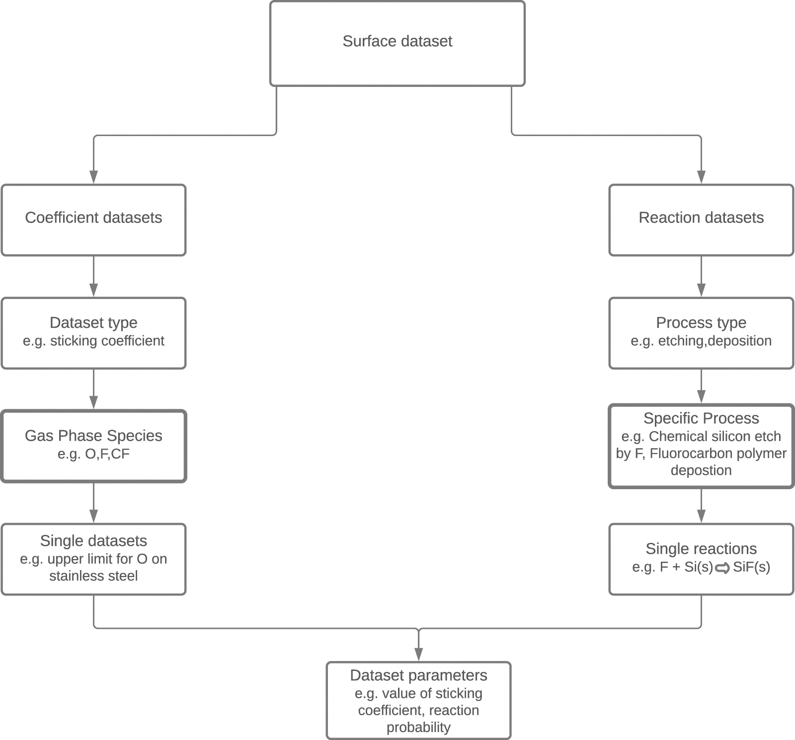
Surface reaction datasets comprise the gas phase species involved and surface species (which follow a similar database structure as the gas phase species) and the, in case of ion-induced processes optionally energy-dependent, coefficient. The data for such reactions are taken from articles describing site-based models [37, 38] or feature profile models [39–41] or both [42], which successfully recreated experimental results. As such, the individual surface reactions on their own do not carry useful information; they only have meaning as part of the entire mechanism. Hence, the individual reactions are grouped into sets of reactions and only these are accessible by the user. Essentially, the database gives access not to individual reactions but to sets of reactions describing a specific etching or deposition process as a whole. The structure of the surface process data is visualized in figure 1.

Figure 1. Hierarchical structure for storing and accessing data on surface processes. The data are presented to the user as collections of individual datasets, indicated by the bolder borders.
Download figure:
Standard image High-resolution imageIt should be noted that data on surface processes usually has much larger uncertainties than, for example, electron collision cross sections. Thus, the QDB surface process data should rather be seen as guide lines, not as definitive data.
Although not completely included in the QDB database yet, energy and angle dependent sputtering yield data play an essential role in determining the profile evolution of surface features during etching and deposition processes, especially corner erosion and redeposition of sputtered or desorbed species from the surfaces of micro/nano-structures [41, 43, 44]. Indeed many experimentally measured sputtering yields as functions of the ion incident energy and angle of incidence have been published and some have been compiled in, e.g., references [45–47]. Most such data are for high-energy ( keV) ion incident energy and single-element ions. For semiconductor plasma processing applications, where low-energy ions are often used to avoid surface damages and incident ions are typically molecular fragments, rather than single-element ions, more data are needed. Yamamura and Tawara derived an empirical formula for the sputtering yields of single-element materials by single-element ions [46], which is available online [48]. Based on the experimental data summarized in reference [45], sputtering yields predicted by machine learning [49] are also available online [50].
2.5. Chemistry generator
While several pre-assembled and validated chemistry sets are available in QDB, they cover only a small fraction of possible plasma modeling applications. As the assembling of application-targeted chemistry sets is a crucial part of any plasma modeling workflow, a Chemistry Generator application was added to the QDB ecosystem to assist with this task. The chemistry generator simply takes the user input in the form of a set of selected feed-stock gases, and traverses the full collisional cascade of species and processes present in QDB. Figure 2 shows a schematic representation of the chemistry generator algorithm.

Figure 2. Schematic flow diagram of the chemistry generator algorithm.
Download figure:
Standard image High-resolution imageHowever, such approach can, if left unmediated, result in a very large number of species and reactions, especially in cases when one or more fragments or products of the feed-gas species has a large number of excited states present in the database. For that reason, users are additionally required to manually select the species of the full QDB reaction network, and their reactions. Species and reactions found in the full reaction network are clustered into several classes, while user has the ability to select all the species/reactions in any given class. Figure 3 shows the screenshot of the chemistry generator GUI in action.

Figure 3. Chemistry generator GUI example. In the first step (not depicted), O2 and Ar feed gases were selected. In the second step (not depicted), only species O, O2, O3, Ar, O+,  and Ar+ were selected, ignoring all the other ions and all the excited species present in QDB. In the third step (depicted), the specific processes are selected, grouped into classes. Once the selection is complete, the chemistry can be downloaded in one of the supported formats, or saved for future reference.
Download figure:
Standard image High-resolution imageAs mentioned above, intervention from the user is currently required in the form of manually selecting individual species and reactions, or their groups. Without such user input, while including all the species and reactions found in the collisional cascade, the chemistry set built will include many redundant species and reactions, making it impractical for plasma modeling applications. In fact, almost all published chemistry sets contain redundant species and reactions [51]. The redundant species and reactions can be eliminated by various chemistry reduction techniques (CRT). Several review papers have dealt with the problem of chemistry reduction [52–56]. While these method were traditionally mostly used by the combustion modeling community, some examples of CRT in plasma modeling applications can be found in the literature [57, 58]. A suitable automatic CRT was also lately developed by Hanicinec et al [59]. We aim to integrate this method into the QDB chemistry generator workflow in the future, making the selection of required species and reactions fully automated, based on user inputs of plasma modeling parameters and conditions.
2.6. Boltzmann solver
A Boltzmann-solver was developed and integrated into the QDB environment to calculate electron energy distribution functions (EEDF) using the cross-sectional data in QDB. This solver is based on the Rockwood formalism [60]. The major difference between the original formalism and the one implemented in QDB is the use of a non-uniform energy grid in the QDB solver. This allows the resolution of fine structures in both cross sections and EEDFs as well as small energy losses (e.g. due to vibrational excitation) in the low-energy range. At higher energies, both cross sections and EEDFs typically show less structures and small energy inelastic collisions are negligible compared to high energy processes such as ionization. Incrementally increasing the energy interval therefore reduces the computational load without reducing the accuracy. For ionization, the colliding electron's energy is reduced by the ionization energy and a new electron is added to the lowest energy bin. For attachment/recombination, the colliding electron is completely removed. Since this changes the number of total electrons in the EEDF, it is renormalized after reaching convergence before calculating rates.
Within the QDB environment, the Boltzmann-solver can be applied to both pre-assembled sets and sets constructed with the chemistry generator. The solver uses all cross-sectional data included in a pre-assembled set or selected by the user in the generator. The user sets the relative densities of the heavy particles and the gas temperature (for the energy transfer by elastic collisions). The Boltzmann-solver is run for several values of the reduced electric field E/N and outputs.
- The EEDFs for the different E/N values
- The effective electron temperature as function of E/N
- The rate coefficients for the used electron collision processes as function of the effective electron temperature.
The data is displayed as graphs in the website and can be downloaded in text format.
2.7. Zero-dimensional model
The Quantemol global model (QGM) has been developed and implemented to the QDB ecosystem, to allow users running fast calculations with both pre-assembled chemistry sets, and dynamically generated chemistry sets (section 2.5). QGM is built around the PyGMol (Python global model) backend, developed by Hanicinec et al for automatic reduction of chemistry sets [59]. It should be noted that the model is approximate, and is more suited for investigating trends and gaining insight into chemistry sets, rather than for quantitative analysis. QGM is outlined in this section, while appendix
The model solves for the set of ordinary differential equations (ODE) consisting of the number density balance equation for each heavy species in the chemistry, in addition to the electron energy density balance equation. The particle density balance equation includes contributions from volumetric reactions, flow, and from diffusion losses (surface sinks) as well as surface sources. The electron energy density balance includes contributions of power from any external sources absorbed by the plasma, elastic and inelastic collisions between electrons and heavy species, generation and loss of electrons in volumetric reactions and power lost by electrons and ions surface losses.
The outputs of the model are the number densities of all the heavy species ni
, number density of electrons ne and the electron temperature Te. The user inputs to the model are plasma parameters, such as power, pressure, feed gas flow rates, dimensions of the plasma and gas temperature. It should be noted that the electron density is not explicitly resolved, but arises from enforcing the charge neutrality. Also, the heavy species temperatures are not resolved by the model, but rather treated as a constant input parameter. Finally, although QDB supports cross-sectional data-sets and has its own Boltzmann solver (section 2.6), the collisional kinetics are parametrized in QGM using the Modified Arrhenius formula, see equations (A.3) and (A.4) in appendix
2.8. Data access and data formats
The data stored in the database is accessible directly via the website, an API, or downloads. Chemistry sets can be downloaded in various formats for plasma simulation packages:
- HPEM [61]: pre-assembled chemistry sets are available via the API, which gives the reactions in HPEM format ready to be copied into the chemistry input file. Dynamic sets can be directly downloaded as an input file. In both cases, some manual corrections might be necessary to make the input compatible with HPEM's internal species and cross-section library.
- QVT: pre-assembled chemistry sets can be directly imported into Quantemol's HPEM based QVT software via an API. Incompatible species and reactions are automatically converted or filtered out, so no manual adjustments need to be made. The API also provides a search for single reactions which can be added to chemistry sets and access to the chemistry generator via the QVT GUI. As with pre-assembled sets, reactions incompatible with HPEM's internal libraries are converted or filtered out automatically.
- COMSOL [62]: an archive with files can be downloaded. This includes a file with the cross sections used in the set and a file with species, both directly importable. Reactions using Arrhenius-coefficient are provided in a separate file and need to be added manually.
- CHEMKIN [63]: ready-to-use input files can be downloaded for both pre-assembled and dynamically created sets.
- CFD-ACE+ [64]: ready-to-use input files can be downloaded for both pre-assembled and dynamically created sets.
- VizGlow [65]: an archive containing a species and a reaction input file which can be directly imported can be downloaded.
Additionally, a file listing the references for all reactions used in a set is available for download in all cases.
Apart from reaction data, the results of the Boltzmann-solver and the global model can be downloaded. In case of the Boltzmann-solver, this is a file listing the effective electron temperature and the rate coefficients for each reaction used for each value of the reduced electric field. For the global model, the download includes a file listing the process parameters and final densities as well as the electron temperature, a list of all reactions used with their Arrhenius parameters, and a .csv file with the transient densities and electron temperature.
The global model is also available as a separate desktop application which downloads the species and reaction data from the QDB website via an API. Constructing chemistry sets and running the model, however, is executed on the local computer.
3. New data
The data available via QDB are constantly being expanded. Below we describe the major extra datasets that have been added since the original release. Data on many individual processes have also been added. We welcome the submission of suitable data for inclusion in QDB.
3.1. Electron collisions with heavy noble gases
Electron collisions with Ne, Ar, Kr, and Xe atoms are a challenging problem, due to the splitting of the  ionic core and the strong term dependence of the valence orbitals in the (np5)n'ℓ excited states. In recent years, the B-spline R-matrix (BSR) method (a close-coupling approach) that may utilize non-orthogonal sets of one-electron orbitals has been very successful to address these issues, since it allows the use of individually optimized term-dependent orbitals sets. A general computer code for non-relativistic and semi-relativistic (Breit–Pauli) BSR was published by Zatsarinny [66], and the method was later extended to a full-relativistic (Dirac–Coulomb) scheme [67]. An overview of the method with a list of applications until 2013 can be found in the Topical Review by Zatsarinny and Bartschat [68]. Updated versions of the BSR and DBSR codes are freely available and can be downloaded from Zatsarinny's GitHub site [69]. Examples using an already compiled and fully installed BSR code can be found on the Atomic, Molecular nd Optical Sciences Gateway [70].
When combined with the R-matrix with pseudo-states (RMPS) approach [71], in which a large number of (discrete) states are squeezed into the R-matrix box and then included in the close-coupling expansion, it is possible to account for the effect of coupling to both the high-lying Rydberg states and the ionization continuum on the cross sections for electron-induced transitions between the low-lying physical bound states. Furthermore, excitation of the positive-energy pseudo-states provides a very good estimate of the ionization cross section. A major advantage of the approach is the consistency associated with a single unitary theory (close-coupling) in which all the results are extracted from the same model.
Using the BSR and DBSR codes, extensive databases have been created for electron collisions with Ne, Ar, Kr, and Xe; these databases have been added to QDB in their entirety. For e-Ne, radiative data [72] as well as cross sections from semi-relativistic [73] and non-relativistic RMPS [74] are available. For e-Ar, radiative data can be found in [75], and the most recent extensive calculation for electron-induced transitions included 500 states in the semi-relativistic model [73]. Finally, for e-Kr and e-Xe, we have full-relativistic results from 69-state (Kr) [76] and 75-state (Xe) [77] models. In the latter calculations, only physical discrete states were coupled.
3.2. Electron collisions with helium
The electron-He collision problem has been treated very successfully by a number of close-coupling with pseudo-states approaches already a long time ago (see, for example, references [78–80]). The previous version of the QDB database contained comparatively old (though likely still reliable) data. Nevertheless, we now include new data based on the 498-state non-relativistic BSR-calculation carried out more recently by Zatsarinny and Bartschat [81] in the context of energy- and angle-differential ionization processes. These data are for elastic scattering, excitation, and ionization from the  S ground state in the energy range from the respective thresholds up to 100 eV. Specifically, we include individual results for the lowest 11 states, i.e., up to (1s3p)1Po, then a sum over pseudo-states below the ionization threshold that is expected to be a good approximation for the combined excitation of the infinite number of discrete Rydberg states, and finally a sum over the remaining pseudo-states that approximates the true ionization cross section. The steps in the energy grid are relatively narrow, but still too coarse to resolve all but the most important resonances just below the first excited level and the ionization threshold. However, the data provided should be sufficient for plasma modelling, where such details are generally not required.
3.3. Reaction data from UMIST and KIDA
Data on reactions from both the KIDA [5, 6] and the UMIST Database for Astrochemistry (UDfA) [82] were added to QDB. Both databases mostly contain heavy particle reactions in form of ion–ion recombination, charge exchange, and various neutral–neutral reactions with some electron collisions, mostly recombination. The databases cover a large range of neutral species as well as positive and negative ions; the focus for both is on astrochemistry, so these species are mostly C and H containing molecules and include some N, O, S, P, and Si containing species as well; there are also few cases of molecules containing F, Fe, Cl, Mg or He.
Both databases were automatically parsed and compared to data already in QDB; missing reactions, species, rate coefficients, and original sources were then added. The KIDA database also contains some evaluation of the reaction data; only rate coefficients evaluated as recommended were added. Adding reactions from these databases led to the addition of three new reaction classifications; heavy-particle electron transfer (HET in table 2), heavy-particle fragmentation (HFR), and heavy-particle radiative association (HRA). It should be noted that both databases also contain rate coefficients in expressions other than the Arrhenius form; since QDB currently does not support these formats, these data were not added to QDB for the time being.
3.4. Electron collisions with iodine
Iodine is being considered as potential fuel for electric propulsion applications in which ionized gas is electrostatically accelerated to generate thrust. This form of thrust generation can significantly increase the payload-to-spacecraft mass ratio as compared to conventional chemical propulsion [83]. The potential use of iodine Hall-effect thrusters [84], in which electrons emitted from a cathode spiral around the thruster axis due to the combination of an axial electric and a radial magnetic field [83, 85], has led to a demand for data on electron collisions with both atomic and molecular iodine. Very recently Ambalampitiya et al [86] published a series of e-I/I2 scattering cross sections computed using R-matrix procedures. These cross sections have now been added to QDB.
3.5. Vibrationally resolved reactions involving N2 and O2
Very extensive datasets of vibrationally-resolved processes involving molecular nitrogen and molecular oxygen have been added to the database. These reactions, which are important for models of atmospheric plasmas, are described in section 4.4 below.
4. Use cases
4.1. Comparison between QGM and LoKI
QGM results were compared against another global model solver, the LisbOn kinetics (LoKI), for the pre-assembled chemistry of oxygen, available at QDB. The analysis adopted two sets of working conditions, considering different gas pressures and electron densities. The following sections present a brief description of the LoKI simulation tool, highlighting differences with respect to QGM and some modifications introduced for the comparison, a summary of the data and working conditions adopted in the simulations, and a discussion of the results obtained.
4.1.1. The LoKI simulation tool
LoKI [87] is a simulation tool developed under MATLAB, that couples two main calculation blocks: (i) a Boltzmann solver (LoKI-B) for the electron Boltzmann equation, released as open-source code licensed under the GNU general public license [88, 89], and (ii) a chemical solver (LoKI-C) for the global kinetic model(s) of pure gases or gaseous mixtures, which solves the zero-dimensional (volume average) number density balance equation for each heavy species in the plasma chemistry. In this workflow, and in contrast to QGM, the balance of the electron energy–density is described by the (homogeneous) electron Boltzmann equation, thus including contributions only due to the power gained/lost from external sources to the plasma and from collisions (elastic, inelastic, superelastic, and non-conservative volumetric reactions). On the other hand, the particle balance equations can include contributions similar to QGM: volumetric reactions, flow and transport mechanisms, including interaction with the surfaces. LoKI includes also a thermal model for the heavy-species, to self-consistently calculate the gas temperature.
LoKI receives the input data via two intuitive parser-files: a setup file defining the physical and numerical working conditions, and a chemistry file detailing the kinetic scheme and data adopted. The latter file was easily constructed for the pre-assembled chemistry of QDB, which involved (i) electron-impact reactions and heavy-species collisions, both described using Arrhenius-type or power-law rate coefficients (depending on the electron temperature or the gas temperature); and (ii) transport + wall-recombination models, for both charged and neutrals species.
Since electron-impact reactions are described here by imposing Te-dependent rate coefficients, there is no need to calculate a non-equilibrium EEDF, hence LoKI-C was used as standalone tool without a coupling to LoKI-B. In this case, and for given plasma parameters (e.g. gas pressure and temperature, electron density, dimensions of the plasma), the code evaluates the densities of the various charged/neutral heavy-species in an iterative procedure that changes the electron temperature (hence the densities of the ions) so as to satisfy the neutrality condition.
LoKI's workflow further includes a pressure cyle where the initial composition of the gas mixture is adjusted to ensure that dissociation/association and wall-interaction mechanisms lead to a final gas pressure equal to the working pressure. In QGM, the pressure regulation adopts a different strategy, by including an additional outflow term in the balance equations of neutral species (see appendix
The major differences between LoKI and QGM are related to the physical models adopted for transport and wall-recombination. For positive ions, number density n+, LoKI describes the rate of wall-losses using

where Λ is the same effective diffusion length defined in (A.14) and  is an effective ambipolar diffusion coefficient, obtained according to the formulation proposed in [90], for charged-particle transport in the presence of several positive ions and a single negative ion with low density. Numerical tests using this model showed considerable deviations between LoKI and QGM results, including different Te-values by more than a factor of 2. For this reason, and also due to the limitations of LoKI's model with respect to negative ions, we have implemented in LoKI the QGM diffusion model for positive ions [91], described in appendix
In LoKI, the transport of neutral species i, number density ni , adopts a model similar to that of QGM, with gain/loss rates given by

with τi the characteristic transport time due to the combined effect of diffusion and recombination at the wall

where Di are multi-component diffusion coefficients calculated adopting Wilke's model [92] and where the total sticking coefficient is identified with a wall-loss probability of recombination of species i, returning to the volume as species k (si = ∑k γik ). Note that equations (6) and (7) correspond to equations (A.12) and (A.13), if Λ is identified with V/A in the first term of (7) and if si /2 is neglected in the second term of (7). Here, the transport of neutral species was described adopting either the expressions presented above (simulations labeled LoKI original) or neglecting the diffusion transport for atomic species using adjusted wall-loss probabilities (simulations labeled LoKI modified), taking

4.1.2. Kinetic scheme and data. Working conditions
QGM and LoKI were compared for the pre-assembled oxygen chemistry available from QDB. Table 3 summarizes the kinetic scheme and data adopted in the simulations, which involve the molecular species O2(X, v = 0–6), O2(a1Δg),  ,
,  , O3(X) and
  ; and the atomic species O(3P), O(1D), O+ and O−.
Table 3. Summary of the oxygen kinetic scheme and data adopted in the simulations. Te is in eV, Tg is in K, and the probabilities s are dimensionless.
| Reaction | Rate coefficient (m−3) |
|---|---|
| Electron impact collisions | |
| e + O2(X, v = 0–1) → e + 2O(3P) |

|
| e + O2(X, v = 1–6) → e + O(3P) + O(1D) |

|
| e + O2(X, v = 0) → e + O2(a1Δg) |

|
e + O2(X, v = 0) → 2e + 
|

|
| e + O2( X, v = 0) → 2e + O(3P) + O+ |

|
| e + O2(X, v = 0) → e + O(3P) + O− |

|
e + O2(a1Δg) → 2e + 
|

|
e +  e + 2O(3P) e + 2O(3P) |

|
| e + O(3P) → 2e + O+ |

|
| e + O(1D) → 2e + O+ |

|
| e + O− → 2e + 2O(3P) |

|
| e + O3(X) → O2(X, v = 0) + O− |

|
e + O3(X) → O(3P) + 
|

|
| e + O2(X, v = 0) → e + O2(X, v = 1) |

|
| e + O2(X, v = 0) → e + O2(X, v = 2) |

|
| e + O2(X, v = 0) → e + O2(X, v = 3) |

|
| e + O2(X, v = 0) → e + O2(X, v = 4) |

|
| e + O2(X, v = 0) → e + O2(X, v = 5) |

|
| e + O2(X, v = 0) → e + O2(X, v = 6) |

|
| Heavy species collisions | |
| 2O2(X, v = 0) → O(3P) + O3(X) |

|
| O2(X, v = 0) + O2(a1Δg) → O(3P) + O3(X) | 2.95 × 10⁻²⁷ |
| O(3P) + O3(X) → 2O2(X, v = 0) | 8.00 × 10⁻¹⁸ exp(−2060/Tg) |
O2(X, v = 0) + O+ → O(3P) + 
|

|
O2(X, v = 0) + O− → O(3P) + 
| 2.50 × 10⁻²⁰ |
| O2(X, v = 0) + O− → e + O3(X) | 5.00 × 10⁻²¹ |
O2(X, v = 0) +  O(3P) + O(3P) + 
| 3.00 × 10⁻²¹ |
O2(X, v = 0) +  e + 2O2(X, v = 0) e + 2O2(X, v = 0) |

|
| O(3P) + O− → e + O2(X, v = 0) |

|
O(3P) +  O2(X, v = 0) + O− O2(X, v = 0) + O−
| 3.30 × 10⁻¹⁶ |
O(3P) +  e + O3(X) e + O3(X) | 1.50 × 10⁻¹⁶ |
O(3P) +  O2(X, v = 0) + O2(X, v = 0) + 
| 3.20 × 10⁻¹⁶ |
O(3P) +  e + 2O2(X, v = 0) e + 2O2(X, v = 0) | 3.00 × 10⁻¹⁶ |
O3(X) + O+ → O2(X, v = 0) + 
| 1.00 × 10⁻¹⁶ |
O3(X) + O− → O2(X, v = 0) + 
|

|
O3(X) + O− → O(3P) + 
| 5.30 × 10⁻¹⁶ |
O3(X) +  O2(X, v = 0) + O2(X, v = 0) + 
| 4.00 × 10⁻¹⁶ |
 + O− → O2(X, v = 0) + O(3P) + O− → O2(X, v = 0) + O(3P) | 1.00 × 10⁻¹³ |
 + O− → 3O(3P) + O− → 3O(3P) |

|
 + +  O2(X, v = 0) + 2O(3P) O2(X, v = 0) + 2O(3P) | 1.00 × 10⁻¹³ |
 + +  2O2(X, v = 0) 2O2(X, v = 0) | 1.00 × 10⁻¹³ |
 + +  2O(3P) + O3(X) 2O(3P) + O3(X) | 1.00 × 10⁻¹³ |
 + +  O2(X, v = 0) + O3(X) O2(X, v = 0) + O3(X) | 1.00 × 10⁻¹³ |
| O+ + O− → 2O(3P) | 1.00 × 10⁻¹³ |
O+ +  O2(X, v = 0) + O(3P) O2(X, v = 0) + O(3P) | 1.00 × 10⁻¹³ |
O+ +  O(3P) + O3(X) O(3P) + O3(X) | 1.00 × 10⁻¹³ |
O+ +  O2(X, v = 0) + 2O(3P) O2(X, v = 0) + 2O(3P) | 1.00 × 10⁻¹³ |
| Transport of heavy species (see text) | |
 + wall → O2(X, v = 0) + wall → O2(X, v = 0) | s+ |
| O+ + wall → O(3P) | s+ |
| O2(a1Δg) + wall → O2(X, v = 0) |

|
| O2(X, v = 1–6) + wall → O2(X, v = 0) |

|
| O(3P) + wall → (1/2)O2(X, v = 0) | sO |
| O(1D) + wall → O(3P) |

|
In table 3, the wall-loss probabilities for ions and for molecular neutral species were taken equal to 1, whereas for atomic neutral species they were either also taken equal to 1 (LoKI original) or adjusted according to the working conditions (LoKI modified).
The simulations considered two sets of working conditions: a high-pressure scenario at p = 104 Pa and ne = 2 × 10¹⁴ m−3, for which the atomic wall-recombination probabilities were set to sO = 7 × 10⁻⁴ and  ; a low-pressure scenario at p = 3 Pa and ne = 1016 m−3, with sO = 0.5 and
  . In both cases, Tg = 500 K.
4.1.3. Results and discussion
Figures 4 and 5 present the densities of the different species considered in the model, for the high and low pressure conditions, respectively, calculated with QGM. For comparison, these figures show also the percent deviation with respect to LoKI results, adopting either the LoKI original or the LoKI modified configurations (see section 4.1.1). In both high/low pressure cases, the plasma is dominated by the vibrational ground-state O2(X, v = 0), exhibiting a low degree of dissociation  ; the most abundant ion species are
  and O−, with similar densities 3–35 times greater than ne.

Figure 4. Density of oxygen species calculated with QGM at high-pressure (blue bars; left scale): p = 104 Pa, Tg = 500 K and ne = 2 × 10¹⁴ m−3. Percent deviation of the results with respect to LoKI calculations (red curves; right scale), obtained adopting the code LoKI original (solid curve) or a LoKI modified version (dashed) with adjusted conditions for the wall-losses of O(3P) and O(1D). In this figure, O2(X) is equivalent to O2(X, v = 0–6), including the full vibrational manifold of the electronic ground-state of molecular oxygen.
Download figure:
Standard image High-resolution image
Figure 5. As in figure 4, but for low-pressure conditions: p = 3 Pa, Tg = 500 K and ne = 1016 m−3.
Download figure:
Standard image High-resolution imageFigures 4 and 5 show a considerable decrease in the deviations between QGM and LoKI when using for the same kinetic scheme but with adjusted conditions for the transport of atomic neutral species (configuration LoKI modified). At high pressure, although the modifications in the transport model are directly aimed at changing the densities of O(3P) and O(1D), they have a global effect upon the gains/losses of all species, contributing to reduce the deviations between LoKI and QGM to values below 20%. The effect extends even to the calculated electron temperature (Te = 1.18 eV, as predicted by QGM), for which deviations of 8.6% and 1.7% are found with respect to LoKI original and LoKI modified, respectively.
At low pressure, electron-impact processes have an increased influence in the kinetic scheme, hence the differences in the calculated electron temperature (4% for both original and modified LoKI configurations, with respect to the QGM prediction of Te = 3.25 eV) are responsible for deviations in the density of species that are still between  , even for LoKI modified. In this case, the modifications in the transport model have an almost exclusive effect upon the densities of O(3P) and O(1D).
The previous analysis highlights the importance of transport models in the overall accounting of the gain/loss rates of species in a plasma. Note that the above agreement between QGM and LoKI was obtained after adopting the same transport model for charged-species, and after neglecting the diffusion transport for atomic species using adjusted wall-loss probabilities (see section 4.1.1).
4.2. Modeling of inductively coupled Ar/NF3/O2 and Ar/NF3 plasmas
Ar/NF3/O2 and Ar/NF3 inductively coupled plasmas (ICP) have been modeled [38, 93] using the reaction set obtained from QDB, see reference [94]. The fluid and hybrid plasma model, CRTRS (see reference [95] and the citations therein), was used for this modeling project. Succinctly, for the results discussed in this paper, the simulations include a frequency-domain electromagnetic model of the ICP source coupled to an electrostatic model of the plasma. The plasma model includes the Poisson equation, continuity equation for all charged and neutral species, momentum equation for ions, and energy equation for electrons. The model considers gas flow using OpenFOAM [96], which is coupled to the plasma model. The Ar/NF3/O2 plasma chemical mechanism is described and used in references [38, 93] and includes 39 species and 308 reactions. The chemistry data (reactions and cross sections) from QDB were used in CRTRS with minor modifications. The Boltzmann equation was solved to compute the reaction rates for electron impact reactions and electron transport coefficient (as a function of the electron temperature Te) using the cross sections provided. The gas and ion temperatures were assumed to be 1000 K in the simulations. The F recombination coefficient (F → F2) was adjusted in the mechanism to 0.004 based on comparison with experimental results (discussed below).
After an initial set of simulations with the full chemistry, a reduced-order chemistry was also developed and simulated. The reduction method is described in detail in reference [59]. In short, the results of one simulation using a global plasma model for given process parameters with the full set is used to rank the species in the set with regards to their influence on the densities of species of interest, e.g. neutral radicals which induce the desired surface interactions. For the reduction itself, the species are then removed in reverse order, i.e. the lowest-ranking species first, and a test run of the global model to establish whether the densities of the specified species of interest stay within a set error margin compared to the full set. If so, the species is considered to be negligible and permanently removed from the set along with all its reactions; if not, the species is reinserted into the chemistry set. In this case, this reduction method was used using QGM for the process conditions detailed below with electrons and atomic F as species of interest to be preserved within 10%. To account for variations in the relative flows, the reduction was carried out independently for three cases (O2 5/10/15 sccm, NF3 15/10/5 sscm, Ar 80 sccm) and only species identified as negligible in all three cases were ultimately removed from the set for the 2D simulations. The reduced chemistry has 23 species and 100 reactions.
We next discuss the two-dimensional modeling of the ICP source described in reference [97]. Modeling was performed using both the full and reduced chemistries. One motivation for modeling this system was the extensive experimental data reported in reference [97]. Before the detailed modeling results are described, we focus on model validation and examine the effect of NF3 fraction in Ar/NF3 plasma on plasma properties. The results for (a) Te 4.5 cm above the center of the bottom electrode, (b) electron density (ne) 4.5 cm above the bottom electrode, and (c) volume averaged F density are plotted in figure 6 as a function of NF3 fraction. Modeling results obtained using the full and reduced chemistries have been compared to experimental data from reference [97]. The plasma power is 140 W and the gas pressure is 30 mTorr in these simulations and experiments. Results using both the full and reduced chemistries generally agree well with experimental measurements. Te in the model is higher than the experiment, which is likely due to the use of the homogeneous Boltzmann equation for computing the EEDF and the reaction rates.

Figure 6. Effect of NF3 fraction in Ar/NF3 plasma on (a) electron temperature (Te) 4.5 cm above the center of the bottom electrode, (b) electron density (ne) 4.5 cm above the bottom electrode and (c) volume averaged F density. Modeling results obtained using the full and reduced chemistry have been compared to experimental results from Kimura and Hanaki [97]. The plasma power is 140 W in these results.
Download figure:
Standard image High-resolution imageWe next focus on a detailed comparison of modeling results from the simulations with full and reduced chemistries. The simulations in figures 7–9 were made for an Ar/NF3/O2 = 80/10/10% gas mixture at 30 mTorr pressure and 140 W plasma power. The gas mixture is assumed to be introduced uniformly below the quartz plate. Te obtained using the full and reduced chemistries is shown in figure 7. Te is highest below the quartz plate as ICP power is mostly coupled to electrons in this region. The densities of a few charged species (electrons, Ar+ ions, and F− ions) are compared in figure 8 using the full and reduced chemistries. Densities of these species peak at the center of the chamber due to diffusion. There is generally good agreement between the full and reduced chemistry models. The overall chemistry is complex with many neutral species. We have compared the densities of a few important neutral radicals (Ar*, F, O*) in figure 9 using the full and reduced chemistries. Chemistry reduction was done to preserve F density, so F density is reasonably close between the two models. So is the density of Ar* and many other neutral species (not shown). However, the O* density highlights that not every quantity will be preserved with the reduced chemistry.

Figure 7. Electron temperature (Te) using the full and reduced chemistries. These simulations have been done for an Ar/NF3/O2 = 80/10/10% plasma at 30 mTorr and 140 W plasma power.
Download figure:
Standard image High-resolution image
Figure 8. Density of (a) electrons (ne), (b) Ar+ ions ( ) and (c) F− ions (nF−) using the full and reduced chemistries. These simulations have been done for an Ar/NF3/O2 = 80/10/10% plasma at 30 mTorr and 140 W plasma power.
Download figure:
Standard image High-resolution image
Figure 9. Density of (a) Ar* (nAr*), (b) F (nF) and (c) O* radicals (nO*) using the full and reduced chemistries. These simulations have been done for an Ar/NF3/O2 = 80/10/10% plasma at 30 mTorr and 140 W plasma power.
Download figure:
Standard image High-resolution imageThe comparison between models with full and reduced chemistries (in figures 7–9) was for one set of conditions. To understand better how well the chemistry reduction works, we have examined the effect of NF3 fraction in Ar/NF3/O2 plasma on spatially averaged densities of electrons, Ar+ ions, and F− ions using the full and reduced chemistries in figure 10. Ar fraction is 80% in these simulations and O2 fraction is 20%—NF3 fraction. The simulations were made at 30 mTorr and 140 W plasma power. There is generally good agreement over the whole range of O2/NF3 gas mixture. Similarly, we look at the effect of NF3 fraction in Ar/NF3/O2 plasma on spatially averaged densities of a few neutral species with the highest concentration (F, N2, O, and NF2) in figure 11. There is generally good agreement between the full and reduced chemistries over the full range of O2/NF3 gas mixture, demonstrating the transferability of the reduction method using a global model to multi-dimensional models.

Figure 10. Effect of NF3 fraction in Ar/NF3/O2 plasma on spatially averaged densities of (a) electrons (ne), (b) Ar+ ions (nAr+) and (c) F− ions (nF−) using the full and reduced chemistries. Ar fraction is 80% and O2 fraction is 20%—NF3 fraction. The simulations have been done at 30 mTorr and 140 W plasma power.
Download figure:
Standard image High-resolution image
Figure 11. Effect of NF3 fraction in Ar/NF3/O2 plasma on spatially averaged densities of (a) F (nF), (b) N2 ( ), (c) O (nO), and (d) NF2 (
 ) using the full and reduced chemistries. Ar fraction is 80% and O2 fraction is 20%—NF3 fraction. The simulations have been done at 30 mTorr and 140 W plasma power.
Download figure:
Standard image High-resolution image4.3. Modeling reactive species formation in He/H2O-based plasma jets at atmospheric pressure
This section illustrates a use case for the chemical reduction method described in reference [59], which is planned for future integration into QDB. In addition, some important aspects to be considered when carrying out reduction of plasma-chemical reaction sets are demonstrated. Here, the formation of reactive species in atmospheric pressure plasma sources, acts as a focus. In general, reactive species formation is of crucial importance for applications in biomedical and surface treatment. Accurate simulation of the absolute densities of these species is challenging due to the complex reaction pathways, which can involve a large number of production and consumption processes. Since the most important processes are often difficult to identify a priori a common approach is to start with a model containing a large number of species and reactions so as to minimise the likelihood of omitting important processes. The requirement to treat large numbers of species means that computationally efficient global models are typically used for such studies. These models allow for detailed insight into the chemical pathways, at the cost of a simplified treatment of the physical processes, such as electron heating. In order to develop simplified sets of chemical reactions for use with more complex physical models, the elimination of species and reactions using chemical reduction techniques is a promising approach. However, any such reduction should be performed carefully in order to ensure that important pathways are not removed accidentally. In addition, the plasma parameter range over which the reduced reaction set (RRS) is valid should be clearly defined as pathways that are unimportant under a certain set of operating conditions may be essential under other operating conditions.
In this section, the chemical reduction method described in reference [59] is applied to the reaction set for He/H2O/O2 originally developed in reference [98] and extended in reference [99]. When used in the global model framework, GlobalKin, developed by Kushner and co-workers [100], this reaction mechanism leads to good agreement with the densities of OH, O and H measured in radio-frequency driven plasma sources, operated in several different geometries, at atmospheric pressure as described in detail elsewhere [98, 99, 101]. In this use case, the chemical reduction and subsequent analysis are carried out in two steps:
- Simulations using the full reaction set are carried out using the QGM in conjunction with the chemical reduction method described in [59].
- Simulations using the RRSs are carried out using GlobalKin.
Reduction of the complete reaction set is carried out for conditions equivalent to those used in figure 7 of [98], where OH densities are measured and simulated as a function of distance along the channel of the plasma source, in the direction of the gas flow. Briefly, the plasma jet used in that work employs a plane-parallel electrode configuration with an electrode separation of 1 mm and electrode areas of (11 × 30) mm. Simulations are carried out using a power-per-unit volume of 18 W cm−3. The gas mixture consisted of He at atmospheric pressure with a water vapor fraction of 0.54% ppm. In [98], pathway analysis demonstrated that the production and consumption processes of OH vary as a function of distance along the gas flow. In order to account for this in the chemical reduction, both the species ranking and the evaluation of the reduced sets with regard to the error induced by removing one species was carried out taking one point in the steady-state regime and one in the regime close to the gas inflow. It should be noted that QGM solves in the time-domain in contrast to the quasi one-dimensional plug flow simulations in GlobalKin; however, this should have limited bearing on the reduction. The criteria used in the reduction consist of a number of simulation outputs that should remain unchanged, in this case to within 10%, before and after reduction. Here, two reductions were carried out. The criteria used for each reduction, as well as the number of species and reactions in the complete and RRSs are summarised in table 4.
Table 4. Summary of the three reaction sets used in this section, and the model outputs that should remain fixed when comparing the original and RRSs.
| Complete reaction set | RRS 1 | RRS 2 | |
|---|---|---|---|
| Fixed quantities | N.A. | Te,ne,nO,nH,nOH |
Te,ne,nO,nH,nOH, , , 
|
| No. species | 46 | 18 | 18 |
| No. reactions | 577 | 90 | 93 |
After completing the reduction process, GlobalKin simulations are carried out, as described in reference [98], with the complete reaction set and each RRS for a variety of different H2O admixtures. For these simulations, the power deposition and plasma dimensions are slightly different to those used in the reduction process. These modified conditions correspond to the those for which OH densities are measured at a fixed location within the plasma jet as a function of H2O admixture, as presented in figure 9 of reference [98]. The densities of several important plasma-produced reactive species in the mixture, OH, H, O and H2O2, predicted by each reaction set are shown in figure 12, which shows that the densities of OH, H and O are well reproduced by both RRSs for H2O admixtures of close to 0.5%. This is expected since the reduction of the complete reaction set is carried out for a gas mixture of ≈0.5% and the densities of OH, H and O are all constrained in the reduction process. For OH and O, the agreement between the complete reaction set and both the reduced sets remains good for all admixtures considered. However, the H densities predicted by the RRS 1 begin to diverge from the complete reaction set for higher H2O admixtures. In the case of H2O2, good agreement is also obtained between the complete reaction set both RRSs for H2O admixtures of close to 0.5%, despite the fact that it is not specifically constrained by the reduction process for RRS 1. However, as for H, the H2O2 density predicted by RRS 1 diverges from that predicted by the complete reaction set at higher H2O admixtures.

Figure 12. Densities of OH, H, O, H2O2 at a distance of 2 cm from the start of the plasma channel, as a function of H2O admixture for the complete reaction set and both RRSs. Power per unit volume = 14 W cm−3.
Download figure:
Standard image High-resolution imageBased on these results, it is clear that the reduction procedure succeeds in generating RRSs that preserve the densities of the constrained species close to the conditions under which the reduction is carried out and that this reduction transfers well between different global models. RRS 2 also allows for a successful prediction of the densities of all species considered over a wider range of admixtures. However, while RRS 1 allows for the OH and O densities to be reproduced over a wider range, the densities of H and H2O2 diverge from the correct solution at higher admixtures.
To obtain greater insight into the origin of these results, the production and consumption pathways of OH are presented in figures 13 and 14. In figure 13, it is observed that RRS 2 reproduces the production pathways of OH found in the complete reaction set almost exactly. For the RRS 1, differences are found when compared to the complete reaction set. Most importantly, reduction 1 leads to the removal of HO2 from the reaction mechanism, which in turn removes the reaction:

Since this reaction plays an increasingly important role in OH formation with increasing distance from the start of the plasma channel, the overall production pathway for OH is changed significantly in comparison to the complete reaction set, even though its density is still preserved.

Figure 13. Relative rates of the major production processes of OH as a function of distance from the start of the plasma channel for the complete reaction set and both RRSs. H2O admixture = 0.5%, power per unit volume = 14 W cm−3. The reaction highlighted in bold denotes a process that is present in the complete reaction set and RRS 2, but not RRS 1.
Download figure:
Standard image High-resolution image
Figure 14. Relative rates of the major consumption processes of OH as a function of distance from the start of the plasma channel for the complete reaction set and both RRSs. H2O admixture = 0.5%, power per unit volume = 14 W cm−3. The reactions highlighted in bold denote processes that are present in the complete reaction set and RRS 2, but not RRS 1.
Download figure:
Standard image High-resolution imageFrom the perspective of OH consumption, shown in figure 14, similar observations can be made. In this case, the RRS 2 also reproduces the consumption pathways of OH found in the complete reaction set almost exactly. However, the absence of HO2 from the RRS 1 leads to the omission of two important OH consumption processes:


As for the production, the omission of these processes modifies the overall consumption dynamic of OH.
From analysis of the production and consumption pathways it can be observed that it is possible to reproduce the densities of OH very accurately using a reaction set that is fundamentally incomplete (RRS 1). In this case, this is made possible due to the similar contributions of HO2 to the production and consumption processes of OH, such that when HO2 is neglected in the reaction set the net effect on the OH density is negligible, under these specific conditions. In general, this underlines the complex nature of model reduction and the importance of comparing formation pathways of important species before and after chemical reduction, in addition to species densities.
4.4. Vibrationally-resolved air chemistry and chemistry reduction
A new chemistry added to the database describes nitrogen/oxygen mixtures [102–104]. This set contains 82 different species and 4663 reactions. The species include also 24 and 15 vibrational levels of N2 and O2, respectively. The vibrational interactions account for 88% of all the reactions. It should be noted that the temperature-dependent rate coefficients of these reactions are not given standard Arrhenius form. These reactions are not included in QDB for the time being but will be added once QDB support for other formats for temperature-dependent rate coefficients is implemented. This chemistry set was used in combination with the zero-dimensional plasma kinetics solver (ZDPlasKin) 0D plasma kinetics solver, which yielded good agreement with experiments for a wide range of conditions and at various feed gas ratios [102–104]. In this example case, we show how one might take a chemistry from the QDB for their own modeling purposes, by means of an initial exploratory study of a different plasma system. The gas phase of a DC driven micro-plasma over water [105] is modeled using the same ZDPlasKin modeling platform. In addition, we show the potential of the chemistry reduction, which will be incorporated into the QDB in the future. The full chemistry and the ZDPlasKin model are briefly described.
4.4.1. Brief summary of the chemistry set
The chemistry set was compiled from various sources. The neutral–neutral and ion–neutral collisions are generally described by rate coefficient expression taken from literature, as described in detail before [102]. The electron impact collisions are described by cross sections mainly taken from the LXCat database [2]. Specifically, the electron impact vibrational (de-)excitation cross sections were taken from the Phys4Entry database instead [7]. Furthermore, the N2–N2, O2–O2 and N2–O2 vibrational–vibrational relaxations and N2–N2, O2–O2, N2–O2 and O2–N2 vibrational–translational (VT) relaxations by Adamovich [106] are included in the chemistry, as well as the VT relaxations of N2–N and O2–O by Esposito [107, 108] and the VT relaxation of N2–O after Guerra and Gordiets [87, 109–114].
4.4.2. ZDPlasKin model setup and comparison against QGM
ZDPlasKin is a FORTRAN 90 based modeling platform to describe non-thermal plasma with complex chemistry [115]. Typically, users write their own master code which incorporates most of the physics. This gives relative freedom to describe a specific plasma system. The master code interacts with the ZDPlasKin module which handles solving the differential equations as well as the coupling with BOLSIG+, the incorporated numerical solver of the Boltzmann equation for the electrons [116]. The DC driven micro-plasma [105] is chosen to be modeled as a simple control volume with perfect mixing in which all species reside only for a short time. The continuity equation then becomes

where P and P0 are the current and initial pressures, respectively. This equation corresponds to volumetric reactions and flow terms of the QGM equation (A.1). However, here we directly set the residence time and the pressure recovery time scale is set equal to this residence time. In addition, unlike in the QGM, this equation is also solved for the electron density and the electron impact rate coefficients are evaluated directly from the EEDF calculated by the coupled Boltzmann solver BOLSIG+. ZDPlasKin does not have an explicit equation to calculate the electron energy (density), instead, the electron energy is the mean electron energy evaluated from the EEDF. To calculate the EEDF from the Boltzmann equation, a (reduced) electric field is required, calculated with [117]

where  is the reduced electric field, N is the gas density and
  is the plasma power density. The electron mobility, μe, is calculated from the (previous) EEDF. This equation assumes that all the plasma power goes into Joule heating of the electrons, and this power principally corresponds to the first term in equation (A.28). ZDPlasKin can also self-consistently calculate the gas temperature, however a fixed gas temperature of 1231 K was chosen based on the experimental setup described. A constant plasma power density of 6276 W cm−3 is used. This corresponds to the experimental plasma, operated at low current. An estimated residence time of 1 ms was chosen based on the small plasma volume [105]. The model is solved until steady state is reached.
4.4.3. Results and discussion
The calculations were performed for gas mixtures ranging from 10/90 to 90/10% N2/O2. The reduction was done based on a selected condition (10/90% N2/O2) and with a focus on N and O atoms and NO and NO2 molecules as the species of interest. The removal of a species from the chemistry was only allowed to change the density of the species of interest by 1%. 38 species could be removed, most of which were ions and electronically excited states. Vibrational levels above the 19th and 5th level of nitrogen and oxygen could also be removed, respectively. This led to the removal of 2571 reactions, 2313 of which involved vibrational levels. Hence, compared to the full set, which consists of 82 different species and 4663 reactions, the reduced set only contains 44 different species and 2350 reactions. In other words, the number of reactions was reduced by 55%. This reduction was found to translate well to the other feed gas ratios. Less restrictive reductions, for example allowing up to 10% change, did not translate equally well to the other feed gas ratios. The resulting electron, N, O, NO and NO2 densities calculated with the full and reduced chemistry are plotted in figure 15. The reduced chemistry gives significantly improved calculation times (30%–40% faster).

Figure 15. Comparison of the full and reduced chemistry sets for different N2 fractions in the feed gas, as calculated with ZDPlasKin.
Download figure:
Standard image High-resolution image
5. Conclusions and future developments
This is the second formal release of the QDB which has seen a significant increase in both the data and functionality provided since the original release in 2017 [10]. It is our intention to continue to expand both features and, in particular, we would welcome any contribution of appropriate data from scientists interested in distributing their results via QDB. We are also exploring the use of machine learning to fill in gaps in knowledge of reactions. However, as the use cases aim to demonstrate, the reactions sets in QDB already provide the necessary data for modeling a range of different plasmas.
This study also illustrates the usefulness of reducing the size of chemistries. In the future we plan to integrate the ranking-based iterative reduction method of Hanicinec et al [59] for automatic selection of relevant species in the chemistry generator as a desktop application of QDB. Our tests above suggest that this reduction works well. Similarly we are aiming for the complete integration of the Boltzmann-solver and QGM. At present the treatment of surface processes remains rather rudimentary and we hope to integrate a site-based surface model with QGM global model, including allowing for self-consistent calculation of surface coefficients used in the plasma model. A further extension of this approach would be the automatic calibration of surface coefficients and unknown rate coefficients to match experimental data.
One new direction we are currently exploring is the role of radiative processes in plasmas. In low pressure plasmas radiative decay of excited states can lead to significant changes in the state populations. We are currently constructing a new lifetime database (LiDa) which will provide information on both lifetimes and radiative decay pathways. For molecules these data are being assembled from the very extensive spectroscopic data for hot molecules provided by the ExoMol database [22].
Acknowledgments
We thank Uwe Czarnetzki, Daniel B Brown, Maria Tudorovskaya, Bridgette Cooper, Peter J Bruggeman, Bastiaan J Braams, Matthew J Goeckner, Alok Ranjan, Geoff Hassall, Khaled Hassouni, E Krishnakumar, Mark J Kushner, Annarita Laricchiuta, Yi-Kang Pu, Julian Schulze, Jung-Sik Yoon, Mi-Young Song, and Nigel Mason, for their contributions to and helpful discussions during this project. Partial funding was received from the UK STFC under Grants ST/M007774 and ST/K004069. Martin Hanicinec would like to thank EPSRC for a CASE studentship under Grant EP/N509577/1. The work of Klaus Bartschat, Kathryn Hamilton, and Oleg Zatsarinny was supported by the United States National Science Foundation under Grants PHY-1803844, OAC-1834740, PHY-2110023, and the XSEDE allocation PHY-090031. The work of Luís L Alves was partially funded by the Portuguese FCT—Fundação para a Ciência e a Tecnologia, under projects UIDB/50010/2020 and UIDP/50010/2020.
Data availability statement
The reactions and species data discussed in this article are available via the QDB database which can be accessed at http://quantemoldb.com.
Appendix A.: Quantemol global model
This section explicitly describes the equations being solved for in the QGM. For clarity, Table A1 summarises all the symbols and quantities used in this section.
Table A1. Summary of symbols used for the documentation of the global model presented.
| Symbol | Unit | Description |
|---|---|---|
| i, k | Index, running over species in a kinetic scheme | |
| i0, i+, i− | Indices i running over neutral, positive and negative species respectively | |
| j | Index, running over reactions in a kinetic scheme | |
| NS | Number of species in a kinetic scheme | |
| ni | m−3 | Number density of the ith species in a kinetic scheme |
| ne | m−3 | Electron number density |
| ϱe | eV m−3 | Electron energy density |
| P | W | Absorbed power |
| p0 | Pa | Desired pressure |
| p | Pa | Instantaneous pressure |
| Qi | sccm | Feed flow for ith species in a kinetic scheme |
| Rp, Zp | m | Plasma dimensions: radius and length |
| V | m3 | Plasma volume |
| Tg | K | Neutral temperature |
| Ti | K | Positive ion temperature |
| Te | eV | Electron temperature |
| kj | m−3+3m s−1 | Reaction rate coefficient of the jth reaction of an order m in a kinetic scheme |
| Rj | m−3 s−1 | Reaction rate of the jth reaction in a kinetic scheme |
| Mcp,j | kg | Mass of the collision partner in jth electron reaction |
| Mi | kg | Mass of the ith species |
| me | kg | Electron mass |
| qi | e | Charge of the ith species |
| e | C | Electron charge |

| m | σ parameter of the Lennard-Jones potential for ith species |

| eV | Electron energy loss due to an inelastic collision j |

| Stoichiometric coefficient of ith distinct species on left-hand side in jth reaction | |

| Stoichiometric coefficient of ith distinct species on right-hand side in jth reaction | |
| aij | Net stoichiometric coefficient of ith distinct species in jth reaction | |
| Aj | m−3+3m s−1 | Arrhenius parameter—pre-exponential factor |
| nj | Arrhenius parameter—exponent | |
| Ea,j | eV | Arrhenius parameter—activation energy |
| Ea,j | K | Arrhenius parameter—activation energy |
| kB | J K−1 | Boltzmann constant |
| si | Sticking coefficient—probability of ith species sticking to a plasma boundary (si ∈ [0, 1]) | |
| rik | Return coefficient—number of ith species returned for each one of stuck
kth species 
| |
| Di | m2s−1 | Diffusion coefficient of ith species |
| Da | m2s−1 | Ambipolar diffusion coefficient |
| Λ | m | Characteristic diffusion length |
| λi | m | Mean free path of ith species |

| m s−1 | Mean speed of ith species |

| m2 | Momentum transfer cross section for ith species scattering on kth species |

| V | Mean sheath voltage |
| nmin | m−3 | Minimal allowed particle density |
| ϱe,min | eV m−3 | Minimal allowed electron energy density |
Particle density balance equation:
The time derivative of all heavy species densities is expressed as a sum of contributions from volumetric processes, flow sources and sinks and surface (diffusion) processes:

The contribution of volumetric reactions is

where  is the density of lth species on the left-hand side of reaction j. The reaction rate coefficient kj
takes form of the modified Arrhenius equation
is the density of lth species on the left-hand side of reaction j. The reaction rate coefficient kj
takes form of the modified Arrhenius equation

for heavy species reactions j (reactions where all the reactants are heavy species) and

for electron processes j (reactions where at least one reactant is an electron). The Arrhenius parameters Aj , nj and Ea,j (or Ea,j ) describe the collisional kinetics of the model.
The contribution of flow to the time evolution of heavy species densities will consist of inflow and outflow terms as well as a term regulating the pressure.

The inflow is expressed as

where

is the inflow expressed in (particles s−1) rather than in (sccm). NA = 6.022 × 10²³ mol−1 is Avogadro constant and Vm = 2.241 × 104 cm3 mol−1 is the molar volume for ideal gas at standard temperature and pressure. The outflow term is set in such a way that only neutrals are leaving the plasma region due to the flow, the neutral species flow rate is proportional to the species density and the total flow rate out of the plasma region is the same as total inflow rate:

where the index i0 runs only over neutral species. And the term regulating the plasma pressure is added to the particle balance equation, accounting for changes in p due to dissociation/association processes and to diffusion losses and surface sources. This term, similarly to the outflow term, only acts upon the neutral species and can be viewed as an addition to the outflow term, or physically as adjusting a pressure-regulation valve between a plasma chamber and a pump, based on the instantaneous pressure.

Here, p is the instantaneous pressure from the state equation for an ideal gas

and τp is a pressure recovery time scale. A value of τp = 10−3 s was found to yield satisfactory results for a wide range of process parameters.
The diffusion contribution toward the particle balance equation is ultimately controlled by the vector of sticking coefficients si and matrix of return coefficients rik and the diffusion model:

The rate of species loss to the plasma boundaries due to diffusion is expressed as

where V and A are plasma volume and plasma boundaries area respectively, while the wall fluxes Γwall,i , as used (among others) by Kushner in GlobalKin [118], is expressed as

where

The diffusion coefficient is calculated separately for neutrals and ions. For positive and negative ions, the diffusion coefficient is the coefficient of ambipolar diffusion in electronegative plasma, as proposed by Stoeffels et al in [91].

Here, γ = Te/Ti and α = ∑ /ne. Di
= 0 for negative ions implies that no negative ions are reaching the plasma boundaries and therefore there are no negative ion diffusion losses. This approximation is justified by the positive plasma potential trapping the negative ions in the plasma bulk. It should be noted that the stated ambipolar diffusion coefficients are only valid for the case of α ≪ μe/μi, where μ are mobilities of electrons and ions respectively. The free diffusion coefficient for heavy species is calculated as
/ne. Di
= 0 for negative ions implies that no negative ions are reaching the plasma boundaries and therefore there are no negative ion diffusion losses. This approximation is justified by the positive plasma potential trapping the negative ions in the plasma bulk. It should be noted that the stated ambipolar diffusion coefficients are only valid for the case of α ≪ μe/μi, where μ are mobilities of electrons and ions respectively. The free diffusion coefficient for heavy species is calculated as

The mean free path λi for all heavy species is

where  is the momentum transfer cross section, and the mean speed
  is the mean thermal speed

where the ion temperature is approximated, as proposed by Lee and Lieberman in [119], by

The momentum transfer cross section  is for the purpose of this model crudely approximated with hard sphere model for neutral–neutral and ion–neutral collisions, and with momentum transfer for Rutherford scattering (as proposed by Lieberman and Lichtenberg in [120]) for the case of ion–ion collisions:

with Debye length

classical distance of closest approach

reduced mass

and the relative speed being approximated by the mean thermal speed

The δik term filters out self-collisions, as collisions between the same species do not affect the species collective behavior

Finally, the free diffusion coefficient for positive ions is approximated by

Each kth species which is lost (or stuck) to the plasma boundary can get returned as ith species, introducing the boundary sources

Electron energy density balance equation:
The balance equation for the electron energy density consists of contributions from the absorbed external power, elastic and inelastic electron collisions, electron production and consumption and contribution from diffusion losses of electrons and ions.

Electron energy density loss rate due to electron collisions is described as

with the electron energy loss for jth reaction ΔEe,j being

and

Rate of change of electron energy density due to generation and loss of electrons is described by

Under a Maxwellian energy distribution assumption, each electron lost through the plasma boundary sheath takes away 2kB Te of energy with it [120], which gives

The total charge flux is kept at zero, yielding

If it is assumed, that ions leave the plasma boundary sheath with the Bohm velocity, each positive ion removed from the plasma takes away  of kinetic energy, as well as sheath voltage acceleration energy [120].

The last open parameter in the system is the mean sheath voltage  , which, according to Lieberman and Lichtenberg [120], can be approximated by

This value of  is only consistent with ICP plasma sources.
Appendix B.: Summary of acronyms and species in QDB
Tables B1, B3 and B2 summarise the neutrals, anions and cations currently considered by QDB, respectively.
Table B1. Summary of neutral, unstateful species currently contained in QDB. Also given is the availability of electron collision data (column A) and heavy particle reaction rates (column B).
| A | B | A | B | A | B | A | B | A | B | A | B | ||||||
|---|---|---|---|---|---|---|---|---|---|---|---|---|---|---|---|---|---|
| Al | ✓ | ✓ | C3F5 | ✓ | ✓ | C5H9 | ✕ | ✕ | CF4 | ✕ | ✕ | F2O | ✓ | ✕ | NP | ✕ | ✓ |
| AlO | ✕ | ✕ | C3F6 | ✓ | ✓ | C5HN | ✕ | ✓ | CF4 | ✓ | ✓ | F3 | ✕ | ✕ | NS | ✕ | ✓ |
| Ar | ✓ | ✓ | C3F7 | ✓ | ✓ | C5N | ✕ | ✓ | CH | ✓ | ✓ | F4 | ✕ | ✕ | NSi | ✕ | ✓ |
| B | ✓ | ✓ | C3F8 | ✓ | ✕ | C5O | ✕ | ✓ | CH2 | ✓ | ✓ | FNO | ✕ | ✓ | Na | ✕ | ✓ |
| BCl | ✓ | ✓ | C3H | ✓ | ✓ | C5S | ✕ | ✕ | CH2F | ✕ | ✓ | FO | ✕ | ✓ | Ne | ✓ | ✕ |
| BCl2 | ✓ | ✓ | C3H2 | ✓ | ✓ | C6 | ✓ | ✓ | CH2F2 | ✓ | ✓ | FO2 | ✕ | ✓ | O | ✓ | ✓ |
| BCl3 | ✓ | ✓ | C3H2N | ✕ | ✓ | C6H | ✓ | ✓ | CH2N2 | ✕ | ✓ | Fe | ✕ | ✓ | O2 | ✕ | ✕ |
| BF | ✓ | ✕ | C3H2O | ✕ | ✓ | C6H10 | ✕ | ✕ | CH2NS | ✕ | ✕ | FeH | ✕ | ✕ | O2 | ✓ | ✓ |
| BF2 | ✓ | ✕ | C3H2S | ✕ | ✓ | C6H12 | ✕ | ✕ | CH2O2 | ✕ | ✓ | H | ✓ | ✓ | O3 | ✓ | ✓ |
| BF3 | ✓ | ✕ | C3H3 | ✓ | ✓ | C6H13 | ✕ | ✕ | CH2S | ✕ | ✓ | H2 | ✓ | ✓ | O3S | ✕ | ✕ |
| BeH | ✕ | ✕ | C3H3N | ✕ | ✓ | C6H14 | ✕ | ✕ | CH2Si | ✕ | ✓ | H2 | ✕ | ✕ | OH | ✓ | ✓ |
| BeH2 | ✓ | ✕ | C3H3Si | ✕ | ✕ | C6H2 | ✕ | ✓ | CH3 | ✓ | ✓ | H2CN | ✕ | ✓ | OP | ✕ | ✓ |
| Br | ✓ | ✓ | C3H4 | ✓ | ✓ | C6H3 | ✕ | ✓ | CH3F | ✓ | ✓ | H2Mg | ✕ | ✕ | OS | ✕ | ✓ |
| Br2 | ✓ | ✓ | C3H4O | ✕ | ✕ | C6H3N | ✕ | ✓ | CH3N | ✕ | ✓ | H2O | ✕ | ✕ | P | ✕ | ✓ |
| BrCl | ✕ | ✓ | C3H5 | ✓ | ✓ | C6H4 | ✕ | ✕ | CH3NS | ✕ | ✓ | H2O | ✓ | ✓ | PH3 | ✓ | ✕ |
| C | ✓ | ✓ | C3H5N | ✕ | ✓ | C6H5 | ✕ | ✓ | CH3O | ✕ | ✓ | H2O2 | ✕ | ✓ | S | ✓ | ✓ |
| C10 | ✓ | ✓ | C3H5Si | ✕ | ✕ | C6H6 | ✕ | ✓ | CH3P | ✕ | ✓ | H2OS | ✕ | ✕ | S2 | ✕ | ✓ |
| C10H | ✓ | ✓ | C3H6 | ✓ | ✓ | C6H7 | ✕ | ✕ | CH3S | ✕ | ✓ | H2P | ✕ | ✓ | SF | ✓ | ✓ |
| C10H2 | ✕ | ✓ | C3H6O | ✕ | ✓ | C6H8 | ✕ | ✕ | CH3Si | ✕ | ✓ | H2S | ✓ | ✓ | SF2 | ✓ | ✓ |
| C10N | ✕ | ✓ | C3H7 | ✓ | ✓ | C6H9 | ✕ | ✕ | CH4 | ✕ | ✕ | H2S2 | ✕ | ✓ | SF3 | ✓ | ✓ |
| C11 | ✕ | ✓ | C3H8 | ✓ | ✓ | C6HN | ✕ | ✓ | CH4 | ✓ | ✓ | H3 | ✕ | ✕ | SF4 | ✓ | ✓ |
| C12 | ✕ | ✕ | C3HN | ✓ | ✓ | C6HSi | ✕ | ✕ | CH4N | ✕ | ✓ | H4 | ✕ | ✕ | SF5 | ✓ | ✓ |
| C12H | ✕ | ✓ | C3HO | ✕ | ✓ | C6N | ✕ | ✓ | CH4NS | ✕ | ✕ | HBr | ✓ | ✓ | SF6 | ✕ | ✕ |
| C12H2 | ✕ | ✕ | C3HS | ✕ | ✓ | C6N2 | ✕ | ✓ | CH4O | ✕ | ✓ | HCHO | ✓ | ✓ | SF6 | ✓ | ✓ |
| C14H10 | ✕ | ✓ | C3HSi | ✕ | ✓ | C7 | ✓ | ✓ | CH4S | ✕ | ✓ | HCN | ✓ | ✓ | SO2 | ✓ | ✓ |
| C2 | ✓ | ✓ | C3N | ✓ | ✓ | C7H | ✓ | ✓ | CH5N | ✕ | ✓ | HCP | ✓ | ✓ | SO2F2 | ✕ | ✓ |
| C2F2 | ✕ | ✕ | C3O | ✕ | ✓ | C7H10 | ✕ | ✕ | CH5NS | ✕ | ✓ | HCl | ✓ | ✓ | SOF | ✕ | ✓ |
| C2F3 | ✓ | ✓ | C3P | ✕ | ✓ | C7H2 | ✕ | ✓ | CHF | ✓ | ✓ | HF | ✓ | ✓ | SOF2 | ✕ | ✓ |
| C2F4 | ✓ | ✓ | C3S | ✕ | ✓ | C7H3 | ✕ | ✕ | CHF2 | ✓ | ✓ | HMg | ✕ | ✓ | SOF3 | ✕ | ✓ |
| C2F5 | ✓ | ✓ | C3Si | ✕ | ✓ | C7H4 | ✕ | ✓ | CHF3 | ✓ | ✓ | HNO | ✕ | ✓ | SOF4 | ✕ | ✓ |
| C2F6 | ✓ | ✓ | C4 | ✓ | ✓ | C7H5 | ✕ | ✕ | CHF3 | ✕ | ✕ | HNSi | ✕ | ✓ | SSi | ✕ | ✓ |
| C2H | ✓ | ✓ | C4F6 | ✓ | ✕ | C7H6 | ✕ | ✕ | CHNO | ✕ | ✓ | HNa | ✕ | ✓ | Si | ✓ | ✓ |
| C2H2 | ✓ | ✓ | C4F7 | ✓ | ✓ | C7H7 | ✕ | ✕ | CHNS | ✕ | ✓ | HNaO | ✕ | ✕ | Si2H4 | ✕ | ✕ |
| C2H2N | ✕ | ✓ | C4F8 | ✓ | ✓ | C7H8 | ✕ | ✕ | CHO | ✕ | ✓ | HO2 | ✕ | ✓ | Si2H5 | ✕ | ✓ |
| C2H2O | ✕ | ✓ | C4H | ✓ | ✓ | C7H9 | ✕ | ✕ | CHO2 | ✕ | ✕ | HO2NO2 | ✕ | ✓ | Si2H6 | ✓ | ✓ |
| C2H2O2 | ✕ | ✕ | C4H10 | ✕ | ✓ | C7HN | ✕ | ✓ | CHS | ✕ | ✓ | HONO | ✕ | ✓ | Si3H7 | ✕ | ✕ |
| C2H2S | ✕ | ✓ | C4H2 | ✕ | ✓ | C7N | ✕ | ✓ | CHSi | ✕ | ✓ | HONO2 | ✕ | ✓ | Si3H8 | ✕ | ✓ |
| C2H2Si | ✕ | ✓ | C4H2N | ✕ | ✕ | C7O | ✕ | ✓ | CN | ✕ | ✓ | HOP | ✕ | ✓ | Si4H10 | ✕ | ✓ |
| C2H3 | ✓ | ✓ | C4H3 | ✕ | ✓ | C8 | ✓ | ✓ | CN2 | ✕ | ✕ | HOS | ✕ | ✕ | Si4H9 | ✕ | ✕ |
| C2H3N | ✕ | ✓ | C4H3N | ✕ | ✓ | C8H | ✓ | ✓ | CNO | ✕ | ✓ | HP | ✕ | ✓ | Si5H11 | ✕ | ✕ |
| C2H3NO | ✕ | ✓ | C4H4 | ✕ | ✓ | C8H2 | ✕ | ✓ | CNSi | ✕ | ✓ | HS | ✕ | ✓ | Si5H12 | ✕ | ✓ |
| C2H3O | ✕ | ✓ | C4H5 | ✕ | ✓ | C8H3 | ✕ | ✕ | CO | ✓ | ✓ | HS2 | ✕ | ✓ | Si6H13 | ✕ | ✕ |
| C2H3Si | ✕ | ✕ | C4H5N | ✕ | ✕ | C8H3N | ✕ | ✓ | CO2 | ✓ | ✓ | He | ✓ | ✓ | Si6H14 | ✕ | ✓ |
| C2H4 | ✓ | ✓ | C4H6 | ✕ | ✓ | C8H4 | ✕ | ✕ | CO2 | ✕ | ✕ | Hg | ✓ | ✕ | Si7H15 | ✕ | ✕ |
| C2H4O | ✕ | ✓ | C4H7 | ✕ | ✕ | C8H6 | ✕ | ✕ | COF | ✓ | ✓ | I | ✕ | ✕ | Si7H16 | ✕ | ✓ |
| C2H4O2 | ✕ | ✓ | C4H8 | ✕ | ✓ | C8HN | ✕ | ✓ | COF2 | ✓ | ✓ | Kr | ✓ | ✕ | Si8H17 | ✕ | ✕ |
| C2H4S | ✕ | ✓ | C4H9 | ✕ | ✕ | C8HSi | ✕ | ✕ | CONH3 | ✓ | ✓ | M | ✓ | ✓ | Si8H18 | ✕ | ✓ |
| C2H5 | ✓ | ✓ | C4HN | ✕ | ✓ | C8N | ✕ | ✓ | COS | ✓ | ✓ | Mg | ✕ | ✓ | Si9H20 | ✕ | ✕ |
| C2H5N | ✕ | ✕ | C4HSi | ✕ | ✕ | C8N2 | ✕ | ✓ | CP | ✕ | ✓ | N | ✓ | ✓ | SiCl | ✕ | ✕ |
| C2H5O | ✕ | ✓ | C4N | ✕ | ✓ | C9 | ✓ | ✓ | CS | ✓ | ✓ | N2 | ✓ | ✓ | SiCl2 | ✓ | ✕ |
| C2H6 | ✓ | ✓ | C4N2 | ✕ | ✓ | C9H | ✓ | ✓ | CSi | ✕ | ✓ | N2 | ✕ | ✕ | SiCl3 | ✕ | ✕ |
| C2HN | ✕ | ✓ | C4P | ✕ | ✓ | C9H2 | ✕ | ✓ | CaF | ✓ | ✕ | N2H | ✕ | ✓ | SiCl4 | ✕ | ✕ |
| C2HN2 | ✕ | ✓ | C4S | ✕ | ✓ | C9H3 | ✕ | ✕ | Cl | ✓ | ✓ | N2H2 | ✕ | ✓ | SiF | ✕ | ✕ |
| C2HO | ✕ | ✓ | C4Si | ✕ | ✓ | C9H4 | ✕ | ✕ | Cl2 | ✓ | ✓ | N2H3 | ✕ | ✓ | SiF2 | ✓ | ✕ |
| C2HO2 | ✕ | ✕ | C5 | ✓ | ✓ | C9HN | ✕ | ✓ | ClHO | ✕ | ✓ | N2H4 | ✕ | ✓ | SiF3 | ✓ | ✕ |
| C2HP | ✕ | ✓ | C5H | ✓ | ✓ | C9N | ✕ | ✓ | ClO | ✓ | ✓ | N2O | ✓ | ✓ | SiF4 | ✓ | ✕ |
| C2HS | ✕ | ✓ | C5H10 | ✕ | ✕ | C9O | ✕ | ✓ | ClO2 | ✕ | ✓ | N2O3 | ✕ | ✓ | SiH | ✓ | ✓ |
| C2HSi | ✕ | ✓ | C5H12 | ✕ | ✕ | CCl | ✕ | ✓ | ClS | ✕ | ✕ | N2O4 | ✕ | ✓ | SiH2 | ✓ | ✓ |
| C2N | ✕ | ✓ | C5H2 | ✕ | ✓ | CCl2 | ✕ | ✕ | Cu | ✓ | ✓ | N2O5 | ✕ | ✓ | SiH2O | ✕ | ✓ |
| C2N2 | ✕ | ✓ | C5H2N | ✕ | ✕ | CCl3 | ✕ | ✕ | 2H | ✕ | ✓ | NF | ✓ | ✓ | SiH3 | ✓ | ✓ |
| C2O | ✕ | ✓ | C5H3 | ✕ | ✕ | CCl4 | ✓ | ✕ | 2H2 | ✕ | ✓ | NF2 | ✓ | ✓ | SiH3O | ✕ | ✓ |
| C2OH6 | ✓ | ✓ | C5H3N | ✕ | ✕ | CF | ✓ | ✓ | 2HC | ✕ | ✕ | NF3 | ✓ | ✓ | SiH4 | ✓ | ✓ |
| C2P | ✕ | ✓ | C5H4 | ✕ | ✓ | CF2 | ✓ | ✓ | 2HCH2NO | ✕ | ✕ | NH | ✓ | ✓ | SiHO | ✕ | ✓ |
| C2S | ✕ | ✓ | C5H5 | ✕ | ✕ | CF3 | ✓ | ✓ | 2HCHO | ✕ | ✓ | NH2 | ✓ | ✓ | SiO | ✓ | ✓ |
| C2Si | ✕ | ✓ | C5H6 | ✕ | ✕ | CF3 | ✕ | ✕ | 2HHN | ✕ | ✓ | NH3 | ✓ | ✓ | SiO2 | ✕ | ✓ |
| C3 | ✓ | ✓ | C5H7 | ✕ | ✕ | CF3I | ✓ | ✕ | 2HN | ✕ | ✕ | NO | ✓ | ✓ | Ti | ✓ | ✕ |
| C3F4 | ✕ | ✕ | C5H8 | ✕ | ✕ | CF3O2 | ✓ | ✕ | F | ✓ | ✓ | NO2 | ✓ | ✓ | Xe | ✓ | ✕ |
| F2 | ✓ | ✓ | NO3 | ✕ | ✓ |
Table B2. Summary of negatively charged, unstateful species currently contained in QDB. Also given is the availability of electron collision data (column A) and heavy particle reaction rates (column B).
| A | B | A | B | A | B | A | B | ||||
|---|---|---|---|---|---|---|---|---|---|---|---|
| Br− | ✓ | ✓ | C5N− | ✕ | ✓ | CN− | ✕ | ✓ |

| ✓ | ✓ |
| C− | ✕ | ✓ |

| ✕ | ✓ | Cl− | ✓ | ✓ |

| ✕ | ✓ |

| ✕ | ✓ | C6H− | ✕ | ✓ | F− | ✕ | ✓ | OH− | ✓ | ✓ |
| C10H− | ✕ | ✓ |

| ✕ | ✓ |

| ✕ | ✓ | S− | ✕ | ✓ |

| ✕ | ✓ | C7H− | ✕ | ✓ | H− | ✓ | ✓ |

| ✕ | ✕ |
| C2H− | ✕ | ✓ |

| ✕ | ✓ | N2O− | ✕ | ✓ |

| ✕ | ✕ |

| ✕ | ✓ | C8H− | ✕ | ✓ |

| ✕ | ✕ |

| ✕ | ✕ |
| C3H− | ✕ | ✓ |

| ✕ | ✓ |

| ✕ | ✕ |

| ✕ | ✓ |
| C3N− | ✕ | ✓ | C9H− | ✕ | ✓ |

| ✕ | ✓ |

| ✕ | ✓ |

| ✕ | ✓ |

| ✓ | ✓ | NO− | ✕ | ✓ |

| ✕ | ✕ |

| ✕ | ✓ |

| ✕ | ✕ |

| ✕ | ✓ |

| ✓ | ✕ |
| C4H− | ✕ | ✓ | CH− | ✕ | ✓ |

| ✕ | ✓ | SiH− | ✕ | ✓ |

| ✕ | ✓ |

| ✕ | ✕ | O− | ✓ | ✓ |

| ✕ | ✓ |
| C5H− | ✕ | ✓ |

| ✕ | ✕ |

| ✕ | ✓ |

| ✕ | ✓ |
Table B3. Summary of positively charged, unstateful species currently contained in QDB.Also given is the availability of electron collision data (column A) and heavy particle reaction rates (column B).
| A | B | A | B | A | B | A | B | A | B | A | B | ||||||
|---|---|---|---|---|---|---|---|---|---|---|---|---|---|---|---|---|---|
| Al+ | ✓ | ✕ | C2P+ | ✓ | ✕ | C4Si+ | ✓ | ✕ |

| ✕ | ✕ |
2

| ✕ | ✕ |

| ✓ | ✓ |
| Ar+ | ✓ | ✓ | C2S+ | ✓ | ✓ |

| ✓ | ✓ | CF3I+ | ✕ | ✕ | F+ | ✓ | ✓ |

| ✓ | ✓ |
| Ar2+ | ✕ | ✕ | C2Si+ | ✓ | ✓ | C5H+ | ✓ | ✓ |

| ✕ | ✕ |

| ✓ | ✓ |

| ✓ | ✓ |

| ✓ | ✓ |

| ✕ | ✕ |

| ✓ | ✓ | CH+ | ✓ | ✓ | F2O+ | ✕ | ✕ | NF+ | ✓ | ✓ |

| ✓ | ✓ |

| ✓ | ✓ | C5H2N+ | ✓ | ✓ | CH+ | ✓ | ✕ | FSi+ | ✓ | ✕ | NF+ | ✕ | ✕ |
| ArH+ | ✓ | ✓ | C3F+ | ✕ | ✕ |

| ✓ | ✓ | CH2+ | ✕ | ✕ | Fe+ | ✓ | ✓ |

| ✓ | ✓ |
| B+ | ✓ | ✕ |

| ✕ | ✕ | C5H3N+ | ✓ | ✕ |

| ✓ | ✓ | H+ | ✓ | ✓ |

| ✕ | ✕ |
| BCl+ | ✕ | ✓ |

| ✕ | ✕ |

| ✓ | ✓ | CH2F+ | ✕ | ✕ |

| ✓ | ✓ |

| ✓ | ✓ |

| ✓ | ✓ |

| ✕ | ✕ | C5H4N+ | ✓ | ✕ |

| ✕ | ✕ |

| ✓ | ✓ |

| ✕ | ✕ |

| ✓ | ✕ |

| ✓ | ✓ |

| ✓ | ✓ | CH2N+ | ✓ | ✓ |

| ✓ | ✓ | NH+ | ✓ | ✓ |
| BF+ | ✓ | ✕ |

| ✓ | ✓ | C5H5N+ | ✕ | ✕ | CH2NO+ | ✓ | ✕ |

| ✓ | ✓ |

| ✓ | ✓ |

| ✓ | ✕ |

| ✓ | ✓ |

| ✕ | ✕ | CH2NS+ | ✓ | ✕ |

| ✕ | ✕ |

| ✓ | ✓ |

| ✕ | ✕ | C3F8 | ✕ | ✕ |

| ✕ | ✕ | CH2O+ | ✕ | ✓ |

| ✕ | ✕ |

| ✕ | ✕ |
| Br+ | ✓ | ✓ | C3H+ | ✓ | ✓ | C5HN+ | ✓ | ✓ |

| ✓ | ✕ | H2F+ | ✓ | ✕ |

| ✓ | ✓ |

| ✕ | ✓ |

| ✓ | ✓ | C5HO+ | ✓ | ✕ | CH2P+ | ✓ | ✓ | H2NO+ | ✓ | ✓ | NO+ | ✓ | ✓ |
| C+ | ✓ | ✓ |

| ✕ | ✕ | C5N+ | ✓ | ✓ | CH2S+ | ✓ | ✕ |

| ✓ | ✓ |

| ✕ | ✕ |
| C2+ | ✕ | ✕ | C3H2N+ | ✓ | ✓ |

| ✓ | ✓ | CH2Si+ | ✓ | ✓ | H2NP+ | ✓ | ✕ |

| ✓ | ✓ |

| ✓ | ✓ | C3H2O+ | ✓ | ✕ | C6H+ | ✓ | ✓ |

| ✓ | ✓ | H2NSi+ | ✓ | ✓ | NP+ | ✓ | ✓ |
| C10H+ | ✓ | ✓ | C3H2S+ | ✓ | ✕ |

| ✓ | ✓ | CH3F+ | ✕ | ✕ | H2Na+ | ✓ | ✕ | NS+ | ✓ | ✓ |

| ✓ | ✓ | C3H2Si+ | ✓ | ✓ | C6H2N+ | ✓ | ✕ | CH3N+ | ✕ | ✕ | H2NaO+ | ✓ | ✕ | NSi+ | ✓ | ✓ |
| C10H2N+ | ✓ | ✕ |

| ✓ | ✓ |

| ✓ | ✓ |

| ✓ | ✕ | H2O+ | ✕ | ✕ | Na+ | ✓ | ✓ |

| ✓ | ✓ |

| ✕ | ✕ |

| ✓ | ✓ | CH3NS+ | ✕ | ✕ | H2O+ | ✓ | ✓ | Ne+ | ✓ | ✕ |

| ✕ | ✓ | C3H3N+ | ✓ | ✓ | C6H4N+ | ✓ | ✓ | CH3O+ | ✓ | ✓ |

| ✓ | ✓ |

| ✕ | ✕ |
| C10HN+ | ✕ | ✕ |

| ✕ | ✕ |

| ✓ | ✓ |

| ✓ | ✓ | H2OP+ | ✓ | ✕ | O+ | ✓ | ✓ |
| C10N+ | ✓ | ✓ | C3H3O+ | ✓ | ✕ |

| ✕ | ✓ | CH3P+ | ✓ | ✕ | H2OSi+ | ✓ | ✕ | O2+ | ✕ | ✕ |

| ✓ | ✕ | C3H3S+ | ✓ | ✕ |

| ✓ | ✓ | CH3S+ | ✓ | ✓ | H2P+ | ✓ | ✓ |

| ✓ | ✓ |

| ✕ | ✕ |

| ✓ | ✓ | C6H7N+ | ✕ | ✕ | CH3Si+ | ✓ | ✓ | H2S+ | ✕ | ✓ |

| ✕ | ✕ |

| ✕ | ✕ |

| ✓ | ✓ | C6H8N+ | ✕ | ✕ |

| ✕ | ✕ | H2S+ | ✓ | ✓ |

| ✕ | ✕ |

| ✕ | ✕ |

| ✕ | ✕ | C6HN+ | ✕ | ✕ |

| ✓ | ✓ |

| ✓ | ✓ |

| ✓ | ✓ |

| ✕ | ✕ | C3H4N+ | ✓ | ✓ |

| ✕ | ✕ | CH4N+ | ✓ | ✕ |

| ✓ | ✓ | OH+ | ✓ | ✓ |

| ✓ | ✓ |

| ✓ | ✓ | C6N+ | ✓ | ✓ | CH4NO+ | ✓ | ✕ | H3NP+ | ✓ | ✕ | OP+ | ✓ | ✕ |
| C2F+ | ✕ | ✕ |

| ✕ | ✕ |

| ✓ | ✓ | CH4NS+ | ✓ | ✕ | H3O+ | ✓ | ✓ | OS+ | ✓ | ✓ |

| ✕ | ✕ | C3H5N+ | ✕ | ✕ | C7H+ | ✓ | ✓ | CH4O+ | ✓ | ✕ | H3OSi+ | ✓ | ✕ | P+ | ✕ | ✓ |

| ✓ | ✓ |

| ✓ | ✓ |

| ✓ | ✓ | CH4P+ | ✓ | ✕ | H3P+ | ✕ | ✓ |

| ✓ | ✓ |

| ✓ | ✓ | C3H6N+ | ✕ | ✓ | C7H2N+ | ✓ | ✓ | CH4Si+ | ✓ | ✓ | H3S+ | ✓ | ✓ | S+ | ✓ | ✓ |

| ✓ | ✓ | C3H6O+ | ✓ | ✓ |

| ✓ | ✓ |

| ✓ | ✓ |

| ✓ | ✓ |

| ✓ | ✓ |
| C2F6 | ✕ | ✕ |

| ✓ | ✓ | C7H3N+ | ✓ | ✕ | CH5N+ | ✓ | ✕ |

| ✓ | ✓ | SF+ | ✕ | ✓ |
| C2H+ | ✓ | ✓ | C3H7O+ | ✓ | ✕ |

| ✓ | ✓ | CH5NS+ | ✕ | ✕ |

| ✓ | ✓ |

| ✕ | ✓ |
| C2H2+ | ✕ | ✕ |

| ✓ | ✕ |

| ✓ | ✓ | CH5O+ | ✓ | ✓ |

| ✓ | ✓ |

| ✕ | ✓ |

| ✕ | ✕ |

| ✓ | ✕ |

| ✕ | ✓ | CH5S+ | ✓ | ✕ | H5Si+ | ✓ | ✓ |

| ✕ | ✓ |

| ✓ | ✓ | C3HN+ | ✓ | ✓ | C7HN+ | ✓ | ✓ | CH6N+ | ✓ | ✕ |

| ✓ | ✓ |

| ✕ | ✓ |

| ✕ | ✕ | C3HO+ | ✓ | ✕ | C7HO+ | ✓ | ✕ | CH6NS+ | ✓ | ✕ |

| ✓ | ✓ |

| ✕ | ✕ |

| ✕ | ✕ | C3HP+ | ✓ | ✕ | C7N+ | ✓ | ✓ | CHF+ | ✕ | ✓ |

| ✓ | ✓ |

| ✕ | ✕ |
| C2H2N+ | ✓ | ✕ | C3HS+ | ✓ | ✓ |

| ✓ | ✓ |

| ✕ | ✓ | HBr+ | ✕ | ✕ |

| ✓ | ✓ |
| C2H2O+ | ✕ | ✓ | C3HSi+ | ✓ | ✓ | C8H+ | ✓ | ✓ | CHNO+ | ✓ | ✓ | HBr+ | ✓ | ✓ | SSi+ | ✓ | ✓ |
| C2H2P+ | ✓ | ✕ | C3N+ | ✓ | ✓ |

| ✓ | ✓ | CHNS+ | ✓ | ✕ | HCHO+ | ✓ | ✓ | Si+ | ✓ | ✓ |
| C2H2S+ | ✓ | ✓ | C3N+ | ✕ | ✓ | C8H2N+ | ✓ | ✕ | CHNSi+ | ✓ | ✓ | HCN+ | ✕ | ✕ |

| ✕ | ✕ |
| C2H2Si+ | ✓ | ✓ | C3O+ | ✓ | ✓ |

| ✓ | ✓ | CHO+ | ✓ | ✓ | HCN+ | ✓ | ✓ |

| ✕ | ✓ |

| ✓ | ✓ | C3S+ | ✓ | ✓ |

| ✓ | ✓ |

| ✓ | ✓ | HCP+ | ✓ | ✓ |

| ✕ | ✕ |
| C2H3N+ | ✓ | ✓ | C3Si+ | ✓ | ✕ | C8H4N+ | ✓ | ✓ | CHOS+ | ✓ | ✓ | HCl+ | ✓ | ✓ |

| ✕ | ✕ |
| C2H3NO+ | ✓ | ✕ |

| ✓ | ✓ |

| ✓ | ✕ | CHP+ | ✕ | ✓ | HF+ | ✓ | ✓ | SiCl+ | ✕ | ✕ |
| C2H3O+ | ✕ | ✓ |

| ✕ | ✕ |

| ✕ | ✓ | CHS+ | ✓ | ✓ | HF+ | ✕ | ✕ |

| ✓ | ✕ |
| C2H3P+ | ✓ | ✕ |

| ✕ | ✕ |

| ✕ | ✕ | CHSi+ | ✓ | ✓ | HHe+ | ✓ | ✓ |

| ✕ | ✕ |
| C2H3S+ | ✓ | ✕ |

| ✕ | ✕ | C8HN+ | ✕ | ✕ | CN+ | ✓ | ✓ | HN2O+ | ✓ | ✕ |

| ✕ | ✕ |
| C2H3Si+ | ✓ | ✓ |

| ✓ | ✓ | C8N+ | ✓ | ✓ | CNH+ | ✕ | ✕ | HNO+ | ✓ | ✓ |

| ✕ | ✕ |

| ✓ | ✓ |

| ✕ | ✓ |

| ✓ | ✓ | CNO+ | ✓ | ✓ | HNP+ | ✓ | ✕ |

| ✕ | ✕ |
| C2H4N+ | ✓ | ✕ | C4H+ | ✓ | ✓ | C9H+ | ✓ | ✓ | CNS+ | ✕ | ✕ | HNS+ | ✓ | ✕ |

| ✓ | ✕ |
| C2H4NO+ | ✓ | ✕ |

| ✓ | ✓ |

| ✓ | ✓ | CNSi+ | ✓ | ✓ | HNSi+ | ✓ | ✓ | SiH+ | ✓ | ✓ |
| C2H4O+ | ✓ | ✕ | C4H2N+ | ✓ | ✓ | C9H2N+ | ✓ | ✓ | CO+ | ✕ | ✕ |

| ✓ | ✓ |

| ✓ | ✓ |

| ✓ | ✕ | C4H2P+ | ✓ | ✕ |

| ✓ | ✓ | CO+ | ✓ | ✓ | HO2S+ | ✓ | ✓ |

| ✓ | ✓ |
| C2H4P+ | ✓ | ✕ |

| ✓ | ✓ | C9H3N+ | ✓ | ✕ | CO2+ | ✕ | ✕ | HO2Si+ | ✓ | ✕ | SiH3N+ | ✓ | ✕ |

| ✓ | ✓ | C4H3N+ | ✓ | ✓ |

| ✓ | ✓ |

| ✕ | ✕ | HOP+ | ✓ | ✓ |

| ✓ | ✓ |

| ✕ | ✕ |

| ✓ | ✓ |

| ✓ | ✕ |

| ✓ | ✓ | HOS+ | ✓ | ✓ |

| ✕ | ✕ |
| C2H5N+ | ✕ | ✕ | C4H4N+ | ✓ | ✓ |

| ✕ | ✕ |

| ✕ | ✕ | HOSi+ | ✓ | ✓ | SiH4N+ | ✓ | ✕ |
| C2H5O+ | ✓ | ✓ |

| ✓ | ✓ |

| ✕ | ✕ |

| ✕ | ✕ | HP+ | ✓ | ✓ | SiO+ | ✕ | ✕ |

| ✓ | ✕ | C4H5N+ | ✕ | ✕ | C9HN+ | ✓ | ✓ |

| ✕ | ✕ | HS+ | ✓ | ✓ | SiO+ | ✓ | ✓ |
| C2H5S+ | ✓ | ✕ |

| ✕ | ✕ | C9HO+ | ✓ | ✕ | COS+ | ✕ | ✓ |

| ✓ | ✓ |

| ✕ | ✓ |

| ✓ | ✓ | C4H6N+ | ✕ | ✕ | C9N+ | ✓ | ✓ | COS+ | ✓ | ✕ | HSSi+ | ✓ | ✓ | Ti+ | ✕ | ✕ |
| C2H6O+ | ✕ | ✕ |

| ✓ | ✓ | CCl+ | ✓ | ✓ | CP+ | ✓ | ✓ | He+ | ✓ | ✓ | ✕e+ | ✓ | ✕ |

| ✓ | ✓ |

| ✕ | ✕ |

| ✕ | ✕ | CS+ | ✕ | ✓ |

| ✓ | ✓ |

| ✓ | ✕ |
| C2H7O+ | ✓ | ✓ |

| ✕ | ✕ |

| ✕ | ✕ | CS+ | ✓ | ✓ | Hg+ | ✕ | ✕ | |||
| C2HN+ | ✓ | ✕ | C4HN+ | ✓ | ✓ |

| ✓ | ✕ | CSi+ | ✓ | ✓ | I+ | ✕ | ✕ | |||

| ✕ | ✓ |

| ✕ | ✕ |

| ✕ | ✕ | CaF+ | ✕ | ✕ | Kr+ | ✓ | ✕ | |||
| C2HO+ | ✓ | ✕ | C4HO+ | ✓ | ✕ |

| ✓ | ✕ | CaF+ | ✓ | ✕ | Kr+ | ✕ | ✕ | |||
| C2HP+ | ✓ | ✓ | C4HP+ | ✓ | ✕ | CF+ | ✕ | ✕ | CaF2+ | ✕ | ✕ | Mg+ | ✓ | ✓ | |||
| C2HS+ | ✓ | ✓ | C4HS+ | ✓ | ✓ | CF+ | ✓ | ✓ | Cl+ | ✓ | ✓ | N+ | ✓ | ✓ | |||
| C2HSi+ | ✓ | ✓ | C4HSi+ | ✓ | ✕ |

| ✕ | ✕ |

| ✓ | ✓ | N2+ | ✕ | ✕ | |||
| C2N+ | ✓ | ✓ | C4N+ | ✓ | ✓ |

| ✓ | ✓ |

| ✓ | ✓ |

| ✓ | ✓ | |||

| ✓ | ✓ |

| ✕ | ✕ |

| ✕ | ✕ | ClO+ | ✓ | ✓ |

| ✕ | ✕ | |||
| C2O+ | ✓ | ✕ | C4P+ | ✓ | ✕ | CF2I+ | ✕ | ✕ | Cu+ | ✓ | ✓ | N2H+ | ✓ | ✓ | |||

| ✓ | ✕ | C4S+ | ✓ | ✓ |

| ✓ | ✓ | 2HH+ | ✓ | ✕ | N2O+ | ✓ | ✓ |
Table B4 summarises the main acronyms used in this paper.
Table B4. Summary of the main acronyms used in the paper.
| AcTC | Active thermochemical tables [15, 16] |
| API | Application program interface |
| BSR | B-spline R-matrix [66] |
| CCCBD | NIST computational chemistry comparison and benchmark database [26] |
| DBSR | Dirac B-spline R-matrix [67] |
| EEDF | Electron energy distribution functions |
| CRT | Chemistry reduction techniques |
| GUI | Graphical user interface |
| HPEM | Hybrid plasma equipment model [61] |
| ICP | Inductively coupled plasma |
| IP | Ionisation potential |
| LiDa | Lifetimes database |
| LoKI | Lisbon kinetics [87] |
| KIDA | Kinetic database for astrochemistry [5, 6] |
| ODE | Ordinary differential equations |
| PyGMol | Python global model |
| QDB | Quantemol database |
| QVT | Quantemol virtual tool |
| QGM | Quantemol global model |
| RMPS | R-matrix with pseudo-states [71] |
| RRS | Reduced reaction set |
| UDfA | UMIST database for astrochemistry [82] |
| ZDPlasKin | Zero-dimensional plasma kinetics solver [116] |