


Abstract
The effect of the magnetic impurities on the charge transport in a magnetic topological ultra-thin film (MTF) is analytically investigated by applying the semi-classical Boltzmann framework through a modified relaxation-time approximation. Our results for the relaxation time of electrons as well as the charge conductivity of the system exhibit two distinct regimes of transport. We show that the generated charge current in a MTF is always dissipative and anisotropic when both conduction bands are involved in the charge transport. The magnetic impurities induce a chirality selection rule for the transitions of electrons which can be altered by changing the orientation of the magnetic impurities. On the other hand, when a single conduction band participates in the charge transport, the resistivity is isotropic and can be entirely suppressed due to the corresponding chirality selection rule. Our findings propose a method to determine an onset thickness at which a crossover from a three-dimensional magnetic topological insulator to a (two-dimensional) MTF occurs.
Export citation and abstract BibTeX RIS
1. Introduction
Topological states as a novel quantum state of matter have attracted a lot of theoretical [1–5] and experimental [6–8] attention in condensed-matter physics. Surprisingly, in contrast to conventional systems, the surface and the bulk of a 3D topological insulator (3DTI) response distinctively to an external electric field, bulk behaves as an insulator while the surface simultaneously posses metallic states which are protected by time reversal symmetry (TRS) or crystalline symmetry [9]. The presence of strong spin–orbit interaction is crucial for the emergence of the topological states. Spin-momentum locking prevents backscattering of electrons off non-magnetic impurities [10, 11] and leads to the quantum anomalous Hall effect [12, 13], topological magnetoelectric effect [14], and a variety of other novel quantum phenomena [15–21].
The conducting electrons on the surface of a 3DTI interact not only with the impurities on the surface but also with the impurities in the bulk. A possible way to decrease the effect of the bulk on the transport of the surface is increasing the surface-to-volume ratio, making the 3DTI thinner. Interestingly, when the thickness of a topological ultra thin film (TTF) is comparable with the decay length of the surface states into the bulk, the wave functions of the top and bottom surface states overlap, which leads to opening a gap in the surface band structure [22–25]. For example, this regime is realized in a thin film of Bi2Se3 when its thickness is less than six quintuple layers [26].
A gap in the surface states of a 3DTI can be induced by breaking the TRS [27, 28]. The TRS can be broken in a 3DTI by exerting an external magnetic field on the system [29–32], by doping the system with magnetic impurities [33–36], and by the magnetic proximity effect when a topological insulator is brought in contact with a ferromagnet [37–42]. Breaking the TRS in a 3DTI destroys the chiral surface states, though cannot remove the degeneracy in the surface states. In contrast to this system, in a magnetic topological ultra-thin film (MTF) the breaking of TRS converts two degenerate massive Dirac cones to two non-degenerate massive Dirac cones.
In this work, we investigate the charge transport of massive Dirac fermions in an MTF in the presence of short-range and randomly placed dilute magnetic impurities. The magnetic impurities are localized scattering centers which force massive Dirac fermions to change their host state. When the magnetic impurities are not aligned fully perpendicular to the MTF, the short-range interaction between them and the conducting electrons is anisotropic, due to the spin-momentum locking of electrons. By applying the semi-classical Boltzmann formalism [43–45], and using a modified relaxation time scheme [46], to truly capture the effect of the present anisotropic interactions, the charge transport of a MTF is investigated.
We address a chirality selection rule which is induced by the magnetic impurities and governs the transitions of electrons between the two non-degenerate massive Dirac cones in a MTF. The chirality selection rule is strongly dependent on the spatial orientation of the magnetic impurities. Then, by changing the tilt angle of the magnetic impurities, the chirality selection rule changes, and consequently, the intraband and interband transitions of conducting electrons will be influenced.
Even though the emergence of the finite size effect gap in a MTF reduces the conductivity of the system. We show in this work how a MTF can provide us with a system in which the massive Dirac fermions generate a dissipation-less charge current in the presence of the magnetic impurities.
When both of the two non-degenerate massive Dirac cones in a MTF are filled with electrons, we found that the extracted charge current is always dissipative. Nevertheless, when only a single band is filled and the magnetic impurities are aligned in-plane, all the possible electronic transitions are forbidden by the chirality selection rule. Remarkably, in consequence, the charge transport across a MTF will be dissipation-less. As it is well known, topological states are usually responsible for dissipation-less charge current. Though, the found zero resistivity in this work originates from trivial topological states. Finally, let us emphasize that the observed fully suppression of the resistivity is a consequence of the hybridization induced gap and hence is not achievable in a 3DTI.
We have organized the rest of this paper as follows. In section 2, we introduce the effective Hamiltonian for a MTF. In section 3, we present and discuss the semi-classical Boltzmann framework along with the modified relaxation time scheme. The obtained results are shown in section 4. In section 4.1, we investigate the charge transport of a MTF in the two-band regime. The charge transport and the resistivity of a MTF in the single-band regime is studied in section 4.2. In section 5, we summarize our findings and conclude with our main results. In appendix
2. Hamiltonian and basic notations
A thick topological film has two surfaces, in which each surface hosts helical gapless states with a specific spin texture (see figure 1). As the thick film becomes thinner the gapless helical states on the opposite surfaces start to hybridize. This hybridization opens a gap of 2Δ in the energy spectrum of the thin film. The size of the energy gap depends on the thickness of the sample [26]. The Hamiltonian describing low energy electrons in a MTF is given by [25, 47]

on the bases of |t ↑⟩, |t ↓⟩, |b ↑⟩, and |b ↓⟩, where t and b denote the top and bottom surface states and ↑, ↓ represent the spin-up and spin-down states, respectively. σi and τi (i = x, y, z) are Pauli matrices in the spin and surface space, respectively. Δm originates from the exchange field of the magnetic dopants, which effectively acts like a Zeeman term and can be changed for instance by using the magnetic proximity effect.

Figure 1. (a) Schematic view of a topological thick film with different spin texture for electrons in the upper and lower surface. (b) A topological thin film with an energy gap of 2Δ opened by hybridization between two opposite surfaces. (c) Illustration of how magnetization M further changes the electronic spectrum of a thin film. (d) Band structure of a Bi2Se3 MTF, for vF = 4.8 (105 m s−1), Δ = 69 meV, and Δm = 35 meV [26].
Download figure:
Standard image High-resolution imageIn this work, we restrict ourselves to the low energy regime and keep terms up to linear order in momentum k. In the presence of the inversion symmetry, we assume that vF is the same for both surface states. Switching to new bases |±↑⟩, |±↓⟩, with  and
and  , H0 reduces to the two decoupled block-diagonal matrix

where hν = ℏ vF(ky σx − νkx σy ) + (Δ + νΔm )σz . The energy dispersion of this Hamiltonian is given by

where s = +/−1 denotes the conduction/valence band. The chiral index ν distinguishes the outer bands (ν =+) from the inner bands (ν =−). The chiral index of the inner band is of the opposite sign to the sign of Δ ⋅ Δm , while the chiral index of the outer band is the sign of Δ ⋅ Δm . The last term in Hν , (Δ + νΔm ), is the mass term. The value of the energy gap for the outer bands is 2|Δ + Δm | and 2|Δ − Δm | for the inner bands, see panel (d) of figure 1.
The chiral basis states that diagonalize the Hamiltonian H0 in equation (2), are  , where
where  ,
,  and the δν,ν' is the Kronecker delta. For a MTF, these so-called surface states emerge in the entire film. Nevertheless, they always lie in the bulk energy gap and therefore can be distinguished from the bulk states.
3. Formalism
In order to find the charge current of massive Dirac fermions in a MTF, the none-equilibrium distribution function of the massive Dirac fermions f
k
should be obtained. We assume that the electric field is weak, hence we consider  , where
  is the equilibrium Fermi–Dirac distribution function. Note,
  does not contribute to the current and
  is linear in the applied electric field
E
. Since only the Fermi electrons contribute to the charge transport, s = +1, we drop the index s in what follows. We apply the semi-classical Boltzmann equation (BE) to find the distribution function of charge carriers in the presence of the external electric field
E
= E(cos χ, sin χ, 0) (see figure 2) and the dilute and randomly placed magnetic impurities. In the regime that the MTF is spatially uniform on scales much larger than the distance between scatterers, the BE reads
is linear in the applied electric field
E
. Since only the Fermi electrons contribute to the charge transport, s = +1, we drop the index s in what follows. We apply the semi-classical Boltzmann equation (BE) to find the distribution function of charge carriers in the presence of the external electric field
E
= E(cos χ, sin χ, 0) (see figure 2) and the dilute and randomly placed magnetic impurities. In the regime that the MTF is spatially uniform on scales much larger than the distance between scatterers, the BE reads

the left side of equation (5) is the collision term. At the steady state the term with the partial time derivative is zero. For electrons that interact only with static impurities but not with each other the collision term is a linear functional of the distribution function. For low energy electrons displaced from equilibrium by a weak homogeneous electric field E , the BE can be rewritten as

where  denotes the non-equilibrium distribution function of electrons residing in band ν and state
k
, and
denotes the non-equilibrium distribution function of electrons residing in band ν and state
k
, and  is the velocity of the electrons. During the scattering, the itinerant electrons scatter off impurities from band ν and state
k
to band ν' and state
k
', with transition rate wνν
'(
k
,
k
'). Fermi's golden rule connects the quantum mechanical scattering matrix Tνν
'(
k
,
k
') with the classical scattering rate wνν
'(
k
,
k
') by
is the velocity of the electrons. During the scattering, the itinerant electrons scatter off impurities from band ν and state
k
to band ν' and state
k
', with transition rate wνν
'(
k
,
k
'). Fermi's golden rule connects the quantum mechanical scattering matrix Tνν
'(
k
,
k
') with the classical scattering rate wνν
'(
k
,
k
') by

The scattering T-matrix is defined as

where |
k
, ν⟩ and  are the eigenstates of the Hamiltonian H0 and H = H0 + Vsc, and Vsc is the scattering potential operator.
  satisfies the Lippmann–Schwinger equation

Within the first Born approximation, the second term in equation (9) can be ignored, which leads to  . Then, the transition rate for the scattering of electrons from their initial state to their final state is given by

where ⟨⟩dis stands for the disorder configuration average. For dilute, random and weak impurities, it is shown that

with nim being the concentration of the present impurities [48]. Let us emphasize that the terms beyond the first Born approximation lead to the anomalous Hall effect and do not contribute to the longitudinal conductivity. For the same reason, we ignore the effect of non-zero Berry curvature in our calculation.

Figure 2. An electron under the presence of an electric field E = E(cos χ, sin χ, 0) scatters off a particular point like magnetic impurity S im = Sim(0, sin θ, cos θ), with initial velocity vk = vk (cos ϕ k , sin ϕ k , 0) and final velocity vk' = vk'( cos ϕ k ', sin ϕ k ', 0).
Download figure:
Standard image High-resolution imageWe model the interaction between an arbitrary electron located at r and a single magnetic impurity at R im as Vsc( r − R im) = Jδ( r − R im) S im ⋅ S e, where S e = hσ/2 stands for the spin of the electron, J is the exchange coupling, and S im = Sim(0, sin θ, cos θ) is the spin of the magnetic impurity, see figure 2. The delta function refers to the short-range nature of the electron-impurity interaction. In the regime of large magnetic spin and weak interaction, we can treat the spin of the magnetic impurities classically. We assume that the magnetic impurities are all aligned in the same direction and as figure 2 illustrates lie in the yz plane, with the z-axis perpendicular to the surface of the MTF.
Depending on how electrons interact with random and point-like impurities, the BE is solved differently. As shown in figure 2 electrons approach the impurities with incident angle ϕ k and scatter off with angle ϕ k ', with the scattering rate wνν '( k , k '). If the scattering potential Vsc scatters electrons isotropically, the relaxation time scheme suggests the following form for the non-equilibrium distribution function at zero temperature [49],

where  and
and  and
and

However, this method does not apply to our work, because, even though the low energy dispersion of a MTF is isotropic, due to the in-plane component of the magnetic impurities the scattering potential is not isotropic. To capture this anisotropy, equation (12) should be modified as follows [46]

where  is the modified relaxation time. In appendix A we quantitatively compare
  with
with  , and
, and  with
with  , proving why this modification is required.
By applying equation (6) for both bands simultaneously, and substituting equation (14) for  , one arrives at the following set of equations,
One practical way to solve this set of the equations is expanding the two unknown functions  in Fourier series, which leads to
Solving equation (16) gives us the Fourier coefficients  ,
,  ,
,  ,
,  . Accordingly, by obtaining these coefficients, one can straightforwardly find the corresponding relaxation times
  . Finally, replacing functions
  and
and  in equation (14) with the found relaxation times yields the distribution function of the electrons with a particular chirality.
Next, the contribution of each band to the conductivity of the MTF can be obtained by

where α and β denote x and y directions. Finally, finding the contribution of all electrons from these two bands yields the total conductivity  .
.
4. Results
We divide our discussion into two parts. In the first part, section 4.1, we assume that both bands are filled with electrons, and both are involved in the charge transport. In this regime the Fermi energy is thus arranged to be above the bottom of the band with plus chirality. In the second part, only the band with minus chirality is filled and contributes to the conductivity, and the Fermi energy lies between the bottoms of the bands. Since our results show completely distinctive features in these two regimes, we present them separately.
4.1. Two-band regime
Being in the two-band regime requires Δ + Δm
⩽ ɛF, where Δ + Δm
is the energy gap of electrons with plus chirality at the Γ point (
k
= 0). Defining  and
and  , the condition
  guarantees that the system is properly driven in the two-band regime.
4.1.1. Transition rate and lifetime of electrons
The transition rate wνν '( k , k ') for electrons determines how likely a scattering event is in which an electron from band ν and state k scatters off a magnetic impurity and ends up being in band ν' and state k', by respecting the conservation of energy. By using the equation (4) the scattering T-matrix Tνν '( k , k ') = ⟨ k , ν|Vsc| k ', ν'⟩ within the first Born approximation is given by
where  ,
,  . Applying equation (11) yields the following result for the transition rate wνν
'(
k
,
k
') of the electrons
. Applying equation (11) yields the following result for the transition rate wνν
'(
k
,
k
') of the electrons
where  . In equation (19), the first and second terms correspond to the intraband and interband scatterings, respectively. Note that while intraband scatterings are isotropic, interband scatterings are anisotropic. Therefore, depending on whether the chirality of electrons is preserved during the scatterings or not, the scattering event is isotropic or anisotropic.
As figure 3 shows, the most and least probable intraband scatterings  are respectively backward, ϕ
k
' − ϕ
k
= ±π, and forward scatterings, ϕ
k
' − ϕ
k
= 2nπ, with n = 0, 1 or −1. However, the most and the least probable interband scatterings occur when ϕ
k
' + ϕ
k
= π or 3π, and ϕ
k
' + ϕ
k
= 2nπ, respectively. Therefore, these two possible scatterings are very distinct. For example, there is always a huge chance for all electrons to be backscattered during an intraband transition, while a few electrons have this chance in an interband scattering. Apart from that, intraband and interband scatterings can be clearly distinguished by their responses to the variation in the direction of the surface magnetization. According to figure 3, changing the direction of the magnetic impurities, from zero to
are respectively backward, ϕ
k
' − ϕ
k
= ±π, and forward scatterings, ϕ
k
' − ϕ
k
= 2nπ, with n = 0, 1 or −1. However, the most and the least probable interband scatterings occur when ϕ
k
' + ϕ
k
= π or 3π, and ϕ
k
' + ϕ
k
= 2nπ, respectively. Therefore, these two possible scatterings are very distinct. For example, there is always a huge chance for all electrons to be backscattered during an intraband transition, while a few electrons have this chance in an interband scattering. Apart from that, intraband and interband scatterings can be clearly distinguished by their responses to the variation in the direction of the surface magnetization. According to figure 3, changing the direction of the magnetic impurities, from zero to  , decreases the transition rate for all intraband scatterings by three orders of magnitude, while it enhances the transition rate for all interband scatterings by two orders of magnitude. Changing the orientation of the magnetic impurities weakens or strengthens different scattering events without changing the profile of the transition rate against ϕ
k
and ϕ
k
.
, decreases the transition rate for all intraband scatterings by three orders of magnitude, while it enhances the transition rate for all interband scatterings by two orders of magnitude. Changing the orientation of the magnetic impurities weakens or strengthens different scattering events without changing the profile of the transition rate against ϕ
k
and ϕ
k
.

Figure 3.
 for Fermi electrons in an intraband scattering (+ ⟼ +) and an interband scattering (+ ⟼ −) versus direction of
k
and
k
', for different orientations of the magnetic impurities θ, and for
for Fermi electrons in an intraband scattering (+ ⟼ +) and an interband scattering (+ ⟼ −) versus direction of
k
and
k
', for different orientations of the magnetic impurities θ, and for  ,
,  .
.
Download figure:
Standard image High-resolution imageEven though in the absence of the external electric field, there is no net charge current across the system, still the electrons travel between the allowed states. Having the transition rate of different scattering events let us calculate how long an electron remains in its host state that helps us to have a broader view of the dynamics of conducting electrons. We can figure out how changing the orientation of the magnetic impurities influences the charge transport over a larger time interval.
By using equation (19) the lifetime of an electron with chirality ν,  , is given by

where  . Note that in the above expression if ν = + then ν' = −, and vice versa. According to the above equation, while
  decreases by increasing θ,
  increases. Therefore, in the absence of an electric field, by increasing θ from 0 to
  , electrons travel from the band with minus chirality to the other band with plus chirality. Finally, all electrons end up having the same lifetime for
  . We can conclude that by changing the orientation of the magnetic impurities, one can change the occupation number of electrons in each band.
Considering that in the absence of an external electric field, there is no preferred scattering event, all transition rates can be weighted equally, as is done in the calculation of the lifetime. But, with the external electric field, the distribution of electrons in different states changes to make some of the possible scatterings more favorable for the charge transport, and suppresses other unfavorable transitions.
4.1.2. Conductivity
The BE takes into account simultaneously both the effect of the electric field and the impurities in the charge transport of the system. As equation (19) implies, charge conduction across a MTF consists of both isotropic and anisotropic transitions. Since these two types of events are correlated, their contributions to the total charge current cannot be separated. Hence, we employ the modified relaxation time scheme for all the possible scattering events in the MTF, to obtain the relaxation times of the conducting electrons. In appendix A the found modified relaxation times are compared with the calculated standard relaxation times, to prove the requirement of the modified relaxation time.
Equation (16) properly captures the anisotropy of scattering events by including the two different modified relaxation times  and
and  for each band and provides us with,

where ![${\tau }_{11}^{\nu c}=\frac{{{\Lambda}}_{{\nu }^{\prime }}\left(1+{\mathrm{tan}}^{2}\enspace \theta \right)+{t}_{0}}{{{\Lambda}}_{\nu }{{\Lambda}}_{{\nu }^{\prime }}\left(1-{\mathrm{tan}}^{4}\enspace \theta \right)+{t}_{0}\left[{t}_{0}+{{\Lambda}}_{\nu }+{{\Lambda}}_{{\nu }^{\prime }}\right]}{\bar{\tau }}_{q}^{\nu }$](https://content.cld.iop.org/journals/1367-2630/22/12/123004/revision3/njpabc989ieqn51.gif) ,
, ![${\tau }_{21}^{\nu s}=\frac{{{\Lambda}}_{{\nu }^{\prime }}\left(1-{\mathrm{tan}}^{2}\enspace \theta \right)+{t}_{0}}{{{\Lambda}}_{\nu }{{\Lambda}}_{{\nu }^{\prime }}\left(1-{\mathrm{tan}}^{4}\enspace \theta \right)+{t}_{0}\left[{t}_{0}+{{\Lambda}}_{\nu }+{{\Lambda}}_{{\nu }^{\prime }}\right]}{\bar{\tau }}_{q}^{\nu }$](https://content.cld.iop.org/journals/1367-2630/22/12/123004/revision3/njpabc989ieqn52.gif) , with
, with ![${\lambda }_{\nu }\left(k\right)=\left[1-{\gamma }_{\nu }^{2}\left(k\right)\right]{\mathrm{cos}}^{2}\enspace \theta $](https://content.cld.iop.org/journals/1367-2630/22/12/123004/revision3/njpabc989ieqn53.gif) ,
,  and
and  .
.
By using equation (17) along with the relaxation times in equation (21), we arrive at following expressions for the two components of the contribution of each band in the total conductivity,
where ![${{\Gamma}}^{\nu }=\frac{{\tilde {\varepsilon }}_{\text{F}}^{2}-{\left(1+\nu {\tilde {{\Delta}}}_{m}\right)}^{2}}{2\left({\tilde {\varepsilon }}_{\text{F}}^{2}+\left[1+\nu {\tilde {{\Delta}}}_{m}\right]\left[1+\nu {\tilde {{\Delta}}}_{m}\enspace \mathrm{cos}\enspace 2\theta \right]\right)}$](https://content.cld.iop.org/journals/1367-2630/22/12/123004/revision3/njpabc989ieqn56.gif) , and
, and  . Also we found that
  . The total conductivities of the system in the x and the y directions can be obtained by
  , and
, and  .
.
4.1.3. The effect of magnetic impurities
The contribution of each band to the total conductivity along with the total conductivity versus θ are shown in figures 4(a) and (b). In panel (a) the Fermi energy lies close to the bottom of the band with plus chirality, and in panel (b) the Fermi energy lies far from the bottom of the band with plus chirality.
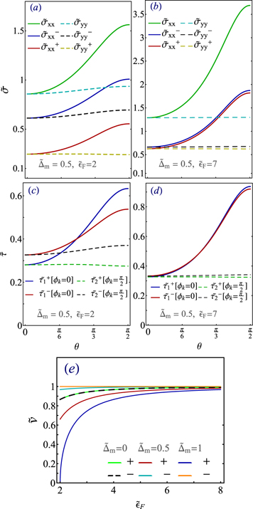
Figure 4. The contribution of each band to the total conductivity and the total conductivity with respect to θ when  and
and  in panel (a), and for
  in panel (b). Panels (c) and (d) are the relaxation times associated to the given conductivities in panel (a) and (b), respectively. (c) The velocity of the Fermi electrons versus
  for different values of
  .
.
Download figure:
Standard image High-resolution imageAs figure 4(a) demonstrates, electrons in the band with minus chirality contribute significantly more to the total conductivity of a MTF, regardless of the direction of the external electric field. When the electric field is applied along the y direction, the value of the relaxation time of electrons with minus chirality,  , the black curve in figure 4(c), is always greater than the value of the relaxation time of electrons with opposite chirality,
  (green curve in the same panel) for any given value of θ. In addition, electrons with minus chirality drift faster than others, see figure 4(e). Since the charge conductivity is only controlled by these two parameters, it can be understood why the contribution of electrons with minus chirality is significantly higher.
When the electric field is applied in the x direction, the same discussion for the dominance of electrons with minus chirality in controlling the total conductivity is valid only when the magnetization orientation is between  . Beyond this regime,
  , the relaxation time of electrons with minus chirality,
  (red curve in figure 4(c)), is shorter than the relaxation time of electrons with plus chirality,
  (blue curve in figure 4(c)). However, even though electrons with minus chirality experience more scattering events than others, in this case, their larger velocity compensates for this. Hence, they again dominate the total conductivity, even in the regime of
  .
.
Moreover, if one fills conduction bands with more electrons, Fermi electrons in bands with opposite chirality end up having very similar relaxation times (see figure 4(d)), regardless of the direction of the external electric field. In addition, as figure 4(e) shows, all electrons conduct charge with the same velocity when  is large. Therefore, as all curves in figure 4(b) demonstrate, all high energy electrons, regardless of their chirality contribute equally to the charge current.
Notice that all the conductivities shown in figures 4(a) and (b) strongly depend on the orientation of the magnetic impurities only when the electric field is applied in the x direction. Surprisingly, the total conductivity and the contribution of each band almost do not vary with θ when the electric field is applied along the y direction.
The weak dependence of  and σyy
on θ can be understood by looking at the spin torque of electrons induced by the magnetic impurities during the scattering time. With an electric field in the y direction, the average momentum of the electrons is also in the y direction. In a 3DTI, the spin of the electrons would be oriented along the x direction due to the spin-momentum locking. In the case of a MTF, the spin can also have a small z component:
and σyy
on θ can be understood by looking at the spin torque of electrons induced by the magnetic impurities during the scattering time. With an electric field in the y direction, the average momentum of the electrons is also in the y direction. In a 3DTI, the spin of the electrons would be oriented along the x direction due to the spin-momentum locking. In the case of a MTF, the spin can also have a small z component:  (the smallest value is reached for electrons with minus chirality ν = − and for high energy electrons). Nevertheless, the spin of the electrons is in this case always approximately perpendicular to the spin of the magnetic impurities (which lies in the yz plane), especially for high-energy electrons and for electrons with negative chirality. Consequently, the torque will be large, and independent of θ, resulting in a small conductivity, almost independent of θ. In case the electric field is along the x direction, the angle between the spin of the electron and the magnetic impurities depends strongly on θ, and thus also the torque, resulting in a strong θ dependence for σxx
.
(the smallest value is reached for electrons with minus chirality ν = − and for high energy electrons). Nevertheless, the spin of the electrons is in this case always approximately perpendicular to the spin of the magnetic impurities (which lies in the yz plane), especially for high-energy electrons and for electrons with negative chirality. Consequently, the torque will be large, and independent of θ, resulting in a small conductivity, almost independent of θ. In case the electric field is along the x direction, the angle between the spin of the electron and the magnetic impurities depends strongly on θ, and thus also the torque, resulting in a strong θ dependence for σxx
.
In appendix B, we systematically measure the degree of sensitivity of the charge current to the direction of the electric field by calculating the anisotropic magneto-resistance (AMR) for each band AMRν and the total AMR
As we explain in appendix
4.1.4. Comparison between the charge conductivities of a MTF and a 3DMT
By comparing the conductivity of a MTF with the conductivity of a 3DMT we can understand how the hybridization between the top and bottom surfaces of a MTF affects the charge conductivity of the system.
In a 3DTI the thickness of the system is much larger than the decay length of the surface states into the bulk and the wave functions of the top and bottom surfaces do not overlap. As a result the 3DTI is a gapless system. In fact the value of the hybridization induced gap Δ decays exponentially as a function of the thickness of the system [26]. In the absence of Δ and Δm the dispersion of a 3DTI consists of two degenerate massless Dirac cones.
We split our discussion into two parts. In the first part, we assume that both the MTF and the 3DMT lack the magnetic dopants that induce the gap Δm . In the second part, we investigate the effect of including Δm . In a TTF two Dirac cones are degenerate, but unlike the dispersion of a 3DTI, these two Dirac cones are always massive, due to the permanent presence of the hybridization induced gap Δ.
In figures 5(a) and (b) we compare the charge conductivity of a TTF and a 3DTI [50] versus  , and for two distinct orientations of the magnetic impurities θ = 0,
  . Here, we assume that the Fermi energy is fixed, and the size of
  can be altered by tunning the Δ. These two panels show that the conductivity of a 3DTI is larger than the conductivity of a TTF, regardless of the direction of the external electric field and the orientation of the magnetic impurities. Decreasing the value of Δ, by increasing the thickness of the system, increases
  and consequently enhances the charge conductivity of the TTF. For large values of
  , which correspond to a significantly thick TTF, the charge conductivity of a TTF is the same as of a 3DTI.
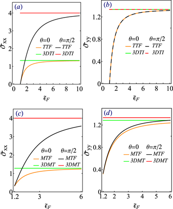
Figure 5. The two components of the conductivity σxx and σyy of a 3DTI and a TTF are shown in panels (a) and (b). Panels (c) and (d) show the two component of the conductivity of a 3DMT and an MTF.
Download figure:
Standard image High-resolution imageAccording to figure 5(a), when the external electric field is applied in the x direction, the charge conductivity of a TTF differs significantly from the charge conductivity of a 3DTI if  . However, this is not true when the spins of the magnetic impurities are perpendicular to the surface of the TTF, i.e. θ = 0. In contrast to the case of
  , figure 5(b) shows that when
  , the difference between the charge conductivity of a TTF and a 3DTI is insensitive to the variations in the orientation of the magnetic impurities. The zero conductivity of the TTF corresponds to the situation in which the Fermi energy lies at the bottom of both bands. It should be noticed that since the Fermi energy is fixed in the conduction band of the 3DTI, its conductivity is always nonzero and constant.
Now, we compare the conductivity of a 3DMT with the conductivity of a MTF. By dopping a 3DTI with strong magnetic dopants, the time-reversal symmetry is broken, which leads to the removal of the surface chiral states and the conversion of the degenerate massless Dirac cones to degenerate massive Dirac cones. However, in contrast to the 3DMT, the breaking of the time-reversal symmetry in a TTF removes also this degeneracy and consequently results in dispersion with two non-degenerate massive Dirac cones, each with distinct chirality, see panel (c) in figure 1.
Figures 5(c) and (d) show that the conductivity of a 3DMT is larger than the conductivity of a MTF. By decreasing the size of the hybridization induced gap, increasing  , the difference between the conductivity of these two systems decreases.
When all the magnetic impurities lie in-plane, it is shown that the conductivity of a 3DMT is insensitive to a change in the size of Δm [50]. In the same condition, due to the hybridization between two opposite surfaces in a MTF, the charge conductivity is highly sensitive to any change in Δm and consequently in the size of the gap 2|Δ ± Δm |. Then, the insensitivity of the charge conductivity of such a system to the gap implies that the system is thick enough, and the finite size effect gap is absent. By altering the thickness of the system, and then again checking the sensitivity of the charge conductivity to the gap, one can determine the critical thickness of the system for which a crossover from a 3DMT to a MTF occurs.
Breaking the time-reversal symmetry decreases the conductivity of the 3DMT, and accordingly increases its resistivity. When the Fermi energy lies in the conduction band, there is always a non-zero resistivity against the charge transport since the degenerate bands both are simultaneously involved in the charge transport. However, in the absence of time-reversal symmetry in a MTF, we can reach a regime in which the resistivity is zero. This will be clarified in detail in section 4.2.
4.1.5. Effect of the gap
In this section, we investigate how changing the size of the gap, 2(Δ + νΔm ), influences the charge transport in a MTF. Here, we keep the value of Δ constant and just change the size of Δm .
The conductivity of each band and the total conductivity of the MTF are plotted versus  , for two critical values of θ, 0 and
  , in a system with constant Fermi energy and Δ, i.e. constant
  . By increasing Δm
, the contribution of electrons with plus chirality decreases while the conductivity of electrons with minus chirality increases, whatever is θ or the direction of the electric field (see figure 6(a)). At
. By increasing Δm
, the contribution of electrons with plus chirality decreases while the conductivity of electrons with minus chirality increases, whatever is θ or the direction of the electric field (see figure 6(a)). At  , the electron occupation number in both bands is the same; see figures 6(c) and (d). When the size of Δm
increases, although the occupation number of electrons with minus chirality increases, the yellow curve in figures 6(c) and (d), the occupation number of conducting electrons with plus chirality decreases and finally reaches zero value at
, the electron occupation number in both bands is the same; see figures 6(c) and (d). When the size of Δm
increases, although the occupation number of electrons with minus chirality increases, the yellow curve in figures 6(c) and (d), the occupation number of conducting electrons with plus chirality decreases and finally reaches zero value at  , see the blue curves in figures 6(c) and (d). The velocity of electrons in both bands interestingly shows a similar trend (see figure 6(e)). Therefore, when the external electric field is applied in the x direction, since the total occupation number of electrons, the red curve in figure 6(c), and the average velocity of electrons, the red curve in figure 4(e), both decrease by increasing the value of
  , the total corresponding conductivity decreases, the red and cyan curves in figure 6(b).

Figure 6. The contribution of each band to the total conductivity (a), and the total conductivity (b) versus  for two critical values of θ and when
  . Panels (c) and (d) show the occupation number of electrons in each band with respect to
  for constant values of θ and
  . Panel (e) shows the velocity of electrons with distinctive chirality against
  .
.
Download figure:
Standard image High-resolution imageWhen the external electric field is applied in the y direction the corresponding conductivity changes too slowly (almost constant) for  , as the total occupation number of electrons changes too slowly, see the black and the green curve in figure 6(b).
4.2. The single-band regime
Here, we investigate the charge transport of a MTF when only the band with minus chirality is filled. To keep the MTF in this regime the Fermi energy can range within Δ − Δm ⩽ ɛF ⩽ Δ + Δm .
If only electrons with minus chirality participate in transport, it is expected that the generated charge current shows some exotic features, which are absent in the two-band regime. To explain why we have such an expectation, let us check the chiral selection rule, which governs the transition of electrons between different states in a MTF. The interaction between an electron and a local magnetic impurity is given by

where
in the spin-chirality Hilbert space. The full Hamiltonian of electrons is  . To check how the chirality of electrons varies through different transitions, one can define the chirality operator in the spin-chirality basis set as
where  , C2 = 1 and
  . We can check the possible conservation of chirality by calculating the commutator
 ![$\left[\mathcal{H},C\right]$](https://content.cld.iop.org/journals/1367-2630/22/12/123004/revision3/njpabc989ieqn100.gif) . Using equations (2), (26) and (25) we arrive at
. Using equations (2), (26) and (25) we arrive at

Since [H0, C] = 0, and ![$\left[{H}_{m}^{\left(1\right)},C\right]=0$](https://content.cld.iop.org/journals/1367-2630/22/12/123004/revision3/njpabc989ieqn101.gif) , one finds
, one finds ![$\left[\mathcal{H},C\right]=\left[{H}_{m}^{\left(2\right)},C\right]$](https://content.cld.iop.org/journals/1367-2630/22/12/123004/revision3/njpabc989ieqn102.gif) . We can conclude that scatterings caused by
. We can conclude that scatterings caused by  has to conserve chirality (corresponding to the intraband transitions), while scatterings caused by
  change the chirality (corresponding to the interband transitions). When all the magnetic impurities are perpendicular to the surface, θ = 0, one finds
  , and consequently only intraband transitions are allowed. For an in-plane orientation of the magnetic impurities, θ = π/2, one finds
  , and only interband transitions can occur. In the single-band regime interband transitions are forbidden because of the conservation of energy. A dissipationless charge current can therefore be expected in the single-band regime for a MTF if θ = π/2.
Now, we calculate the resistivity of a MTF in this regime to prove this exciting finding. Since in what follows, we discuss the charge transport of just electrons with minus chirality, we drop the chirality index for the sake of convenience. The found transition rate for the electrons with minus chirality is

where ϕ− = ϕ
k'
− ϕ
k
,  ,
,  . As equation (28) shows, the out of plane component of the magnetic impurities controls the transition of electrons. By weakening this component of the magnetic impurities, the scattering probability decreases for all possible scattering events, and eventually vanishes at
  . In other words, if all the magnetic impurities lie in-plane, electrons stay forever in their host state and never scatter into the other states.
Substituting equation (28) in equation (16) yields the following relaxation time for electrons in this regime

This indicates that the relaxation time of electrons increases by increasing θ and diverges at  , which once again confirms that electrons with minus chirality do not encounter any scattering events in this situation.
Replacing the relaxation time in equation (17) with equation (29) yields the following charge conductivity of electrons in this regime
Accordingly, the resistivity matrix will be

where ![${\rho }_{xx}\left[\frac{h}{{e}^{2}}\right]={\rho }_{yy}\left[\frac{h}{{e}^{2}}\right]={\rho }_{0}\enspace {\mathrm{cos}}^{2}\enspace \theta \enspace \frac{3{\tilde {\varepsilon }}_{\text{F}}^{2}+{\left({\tilde {{\Delta}}}_{m}-1\right)}^{2}}{{\tilde {\varepsilon }}_{\text{F}}^{2}-{\left({\tilde {{\Delta}}}_{m}-1\right)}^{2}}$](https://content.cld.iop.org/journals/1367-2630/22/12/123004/revision3/njpabc989ieqn111.gif) , and
, and  .
.
This result also shows another remarkable finding: the conductivity of a MTF in the single-band regime is always isotropic, σxx = σyy , in contrary to the extracted conductivity for this system in the two-band regime, equation (22). The anisotropy in the conductivity for a MTF in the two-band regime originates from the in-plane component of the magnetic impurities. However, in the single-band regime, the in-plane component of the magnetic impurities is not able to scatter electrons, see equation (28), and consequently, the calculated conductivity for this regime is isotropic.
Figure 7(a) shows this resistivity as a function of θ. It decreases by increasing θ, and indeed eventually vanishes at  , regardless of the value of
  , and
, and  . This provides us with another criterion to distinguish the single-band regime from the two-band regime in the charge transport of a MTF. Since Δ is constant, the value of the energy gap 2|Δ − Δm
| decreases by increasing the value of Δm
. Therefore, by increasing the value of Δm
, or
. This provides us with another criterion to distinguish the single-band regime from the two-band regime in the charge transport of a MTF. Since Δ is constant, the value of the energy gap 2|Δ − Δm
| decreases by increasing the value of Δm
. Therefore, by increasing the value of Δm
, or  , the conductivity increases, and consequently, the corresponding resistivity decreases (figure 7(b)).

Figure 7. The resistivity of an MTF in the single-band regime versus θ (a), and  (b).
(b).
Download figure:
Standard image High-resolution imageFinally, we want to stress that the charge current in this regime stays dissipationless as long as the chirality selection rule remains unchanged. The presence of extra effects can modify the band dispersion and may break the chirality selection rule, making the charge current dissipative. For example, an in-plane magnetic field causes the band dispersion to be an asymmetric, tilted Dirac cone [51, 52]. Hence, it can generate a finite resistivity in this regime. A perpendicular electric field can also modify the transition selection rule by breaking the inversion symmetry [53], even though the dispersion relation remains symmetric.
5. Conclusion
The charge transport of a MTF is investigated by applying the Boltzmann semi-classical formalism along with a modified relaxation time scheme. Two distinct regimes are identified depending on whether both conduction bands are engaged in the charge transport or not. For each regime, the relaxation times of electrons and the charge conductivity of the system are found analytically. When both conduction bands are filled with electrons, the generated charge current is anisotropic. In contrast to this regime, we found that the conductivity of a MTF is isotropic when only a single conduction band is involved in the transport. The extracted conductivity in both of these regimes is highly sensitive to the orientation of the magnetic impurities, the size of the energy gap, and the value of the Fermi level.
Interestingly, the magnetic impurities induce a chirality selection rule which governs the transitions of electrons during different scattering events. When both of the conduction bands are filled, the charge current is always dissipative. Nevertheless, when only a single band is occupied, the chiral selection rule forbids all the transport channels for electrons if the magnetic impurities lie in-plane. In consequence, the charge transport across a MTF will be surprisingly dissipation-less.
This work provides a criterion to specify a crossover from a 3DTI to a MTF. When all the magnetic impurities are in-plane in a 3DMT, the measured charge conductivity is insensitive to the gap. In contrast to this system, in a MTF with in-plane magnetic impurities, the charge conductivity is highly sensitive to the gap. Therefore, by altering the thickness of the system, and then again checking the sensitivity of the charge conductivity to the gap, one can determine the critical thickness of the system for which a crossover from a 3DMT to a MTF occurs.
Acknowledgments
MZ acknowledges support from the U.S. Department of Energy (Office of Science) under Grant No. DE-FG02- 05ER46203.
Appendix A.: Comparing the standard relaxation time with the modified relaxation time
In this appendix we quantitatively compare our calculated modified relaxation times with usual standard relaxation times. By making this comparison, we show the importance of using the modified relaxation time in our work.
By applying the equations (19) and (13) the standard relaxation time of an electron in band ν and state k will be

The standard relaxation time scheme is applicable only when all the scattering events are isotropic, in which the transition rate depends only on the angle between
k
and
k', Δϕ = ϕ
k
− ϕ
k'
. Consequently, the corresponding relaxation time depends only on the magnitude of
k
, not on its direction. Nevertheless, the expression in equation (A.1) contradicts this point. The apparent contradiction implies that the system is not isotropic. However, we can ignore this contradiction and still follow this approach in order to just make an estimation for the relaxation time, without going through a lengthy calculation that solving equation (16) requires. We will demonstrate that the value of the standard relaxation times  deviate too much from the modified relaxation times
  in a system with in-plane magnetization.
Figure A1 quantitatively compares  , with
  and
and  . In all panels dashed and solid curves correspond to the electrons with minus and plus chirality, respectively. The red and cyan curves in panels (a)–(c) are
  and
and  , and in panels (d)–(f) are
  and
and  , respectively.
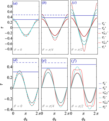
Figure A1.
 (cyan),
  (red), and
  (blue) are shown versus ϕ
k
for three different orientations of the magnetic impurities. In all panels dashed and solid curves correspond to the electrons with minus and plus chirality, respectively.
(blue) are shown versus ϕ
k
for three different orientations of the magnetic impurities. In all panels dashed and solid curves correspond to the electrons with minus and plus chirality, respectively.
Download figure:
Standard image High-resolution imageAs equation (19) indicates, when the MTF has a perpendicular magnetization, all electrons keep their chirality unchanged during a scattering event and encounter an isotropic transition. Therefore, it is obvious why these two methods produce the same relaxation times. However, when one increases the in-plane component of the magnetization, the standard relaxation time starts to deviate from the other accurate ones. At  , the value of the standard relaxation time differs too much from the accurate value, in all panels. Apart from that, since the external electric field causes electrons to leave their band, the lifetime of most electrons (blue curves in this figure) is greater than their relaxation time. In addition, changing the orientation of the magnetic impurities from θ = 0 to
  makes electrons with minus chirality distinguishable from those with plus chirality by referring to their relaxation times.
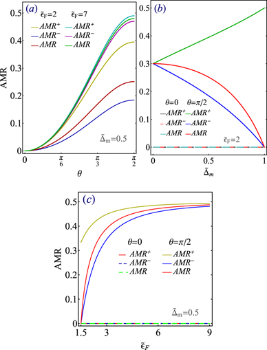
Appendix B.: Anisotropic magneto-resistance
In this appendix, we investigate the dependency of the generated charge current in a MTF on the direction of the electric field. The external electric field affects the momentum of electrons, and due to the large spin-momentum locking, it consequently affects the spins of electrons. On the other hand, since the spin of electrons interacts with the spin of magnetic impurities, the external electric field subsequently influences the strength of scatterings and consequently the conductivity of the system. Then, it is obvious why changing the direction of the external electric field can strongly affect the conductivity of a MTF.
By using equation (22), we find

According to equation (B.1), for a MTF with a fully out of plane magnetization, θ = 0, the value of AMRν
is zero for both bands and as we already knew, the system is isotropic. On the other hand, for a MTF with a completely in-plane magnetization, ![${\text{AMR}}^{\nu }\left[\theta =\frac{\pi }{2}\right]={{\Gamma}}^{{\nu }^{\prime }}$](https://content.cld.iop.org/journals/1367-2630/22/12/123004/revision3/njpabc989ieqn132.gif) . Accordingly, the value of the AMRν
for each band ranges from 0 to Γν
'. According to equation (B.1), AMRν
depends on Γν
', which implies that the anisotropy in the conductivity of a particular band originates from the interband scatterings, in agreement with equation (19).
. Accordingly, the value of the AMRν
for each band ranges from 0 to Γν
'. According to equation (B.1), AMRν
depends on Γν
', which implies that the anisotropy in the conductivity of a particular band originates from the interband scatterings, in agreement with equation (19).
Figure B1(a) compares the AMR with AMR+ and AMR−, for a particular value of θ, with  = 2, 7, and
  = 0.5. All curves increase by increasing θ, regardless of the value of
  and the chirality of the electrons. This is due to the fact that the strength of interband scattering, which is responsible for the anisotropy, increases by increasing θ, see equation (19).
Figure B1. The AMR, AMR−, AMR+ with respect to  ,
,  and θ.
Download figure:
Standard image High-resolution image
As figure 4(a) demonstrates, when the Fermi energy lies on the bottom of the band with plus chirality,  ,
,  , though
  , which eventually leads to AMR+ ≳ AMR−, (see figure B1(a)). Hence, for this case, electrons with plus chirality play the important role in the anisotropy of the derived conductivity of the MTF.
For the case of  , (figure 4(b)),
  and
and  , which results in AMR+ ≃ AMR−. Therefore, electrons that reside in the top of their host bands have the same share in generating the anisotropy in the conductivity.
The red and green curves in figure B1(a) demonstrate that the anisotropy in the total conductivity increases by increasing θ. This is due to the fact that σxx diverges greatly from σyy by increasing θ (see figures 4(a) and (b)).
Now, we assume that all the magnetic impurities are aligned in a fixed particular direction, and consider that the position of the Fermi energy is also fixed. Note that the value of the hybridization induced gap Δ is fixed in this work. However the size of the energy gap 2|Δ + νΔm | can be altered by changing the value of Δm . In what follows, we investigate how the degree of the anisotropy in the conductivity of each band and also the total conductivity can be controlled by tuning the size of the energy gap.
Figure B1(b) shows AMR−, AMR+ and AMR versus  , for two values of θ and with
  . As expected, the contribution of each band and also the total conductivity is isotropic when all magnetic impurities are aligned perpendicular to the surface of a MTF. In case of having all the magnetic impurities aligned in-plane, AMR− and AMR have a decreasing trend versus
  , while AMR+ has an increasing trend against
  .
.
When  , based on equation (19), just interband scatterings are possible for electrons, regardless of their chirality. In addition, as equation (19) indicates, the transition rate ωνν
'(
k
,
k
') for an interband scattering is symmetric with respect to the chirality index. Accordingly, the probability of an interband scattering is independent of the chirality of electrons. However, during an interband transition, the band with minus chirality can host much more electrons. Therefore, the produced conductivity by electrons with plus chirality is much more anisotropic compared to the generated current by electrons with minus chirality, see figure B1(b). Regarding the anisotropy in the total charge current, because the transition rate of all interband scatterings decreases with increasing
, based on equation (19), just interband scatterings are possible for electrons, regardless of their chirality. In addition, as equation (19) indicates, the transition rate ωνν
'(
k
,
k
') for an interband scattering is symmetric with respect to the chirality index. Accordingly, the probability of an interband scattering is independent of the chirality of electrons. However, during an interband transition, the band with minus chirality can host much more electrons. Therefore, the produced conductivity by electrons with plus chirality is much more anisotropic compared to the generated current by electrons with minus chirality, see figure B1(b). Regarding the anisotropy in the total charge current, because the transition rate of all interband scatterings decreases with increasing  , the amount of produced anisotropy decreases (the red curve in figure B1(b)).