Global Seismic Noise Entropy

Introduction

The preparation processes for strong earthquakes are accompanied by changes in the statistical properties of seismic noise (Lyubushin, 2012, 2013, 2015, 2017, 2018, 2020c). As shown in (Berger et al., 2004, Fukao et al., 2010, Koper and de Foy, 2008, Koper et al., 2010; Ardhuin et al., 2011; Aster et al., 2008; Friedrich et al. 1998; Grevemeyer et al., 2000; Kobayashi, Nishida, 1998; Nishida et al., 2008, Nishida et al., 2009, Stehly et al., 2006; Rhie, Romanowicz 2004, 2006; Tanimoto, 2001, 2005), the main source of energy of seismic noise is ocean waves affecting the shelf and coast, as well as variations in atmospheric pressure on the Earth's surface arising from the movement of cyclones. In (Lyubushin, 2012; Lyubushin, 2013; Lyubushin, 2018; Lyubushin, 2020c), changes in the temporal and spatial structure of seismic noise in Japan and California, which are precursors of strong earthquakes, are identified. The article investigates the properties of seismic noise entropy from continuous records of the global network of broadband seismic stations for 23 years, 1997–2019. The main goal of the article is to evaluate the spatial and temporal correlations of entropy changes and the relationship between the entropy of seismic noise and the length of day (LOD) parameter (day length), which is a sequence of day length values and a characteristic of the Earth’s irregularity of rotation, and to estimate the possible trigger effect of the irregularity of the Earth’s rotation on the occurrence of the strongest earthquakes.

Seismic Noise Data

The used data present vertical components of continuous records of seismic noise with a sampling time interval of 1 s which were downloaded by request from the site of Incorporated Research Institutions for Seismology by the address http://www.iris.edu/forms/webrequest/ from 229 broadband seismic stations of the following three networks:

Global Seismographic Network: http://www.iris.edu/mda/_GSN.

GEOSCOPE: http://www.iris.edu/mda/G.

GEOFON: http://www.iris.edu/mda/GE.

Seismic noise records with a sampling rate of 1 Hz (LHZ records) were considered for 23 years of registration (from January 1, 1997, to December 31, 2019). These data were converted to a time series with a time step of 1 min by calculating averages for successive time slices of 60 s. Orthogonal wavelets were used to calculate daily entropy values for low-frequency seismic noise.

An important issue in the application of the technique used to study the properties of seismic noise is that, formally, the frequency range of signals recorded using seismic sensors does not include periods from two to about 1,000 min, which are actually investigated after the transition to a time step of 1 min at a time interval of 1 day length. The question arises about the legality of the transition to such a low-frequency region of the seismic signal records. We believe that when solving the problems of geophysical monitoring, there is a fundamental possibility of a wider application of broadband seismic equipment, which exceeds the formal limitations on the operating frequency band, which is traditionally used in the study of individual earthquakes. The basis for this assumption is the estimates of the power spectra of seismic signals after the transition to a time step of 1 min and even 1 h, shown in Figure 1 for two seismic stations. In Figures 1A,B, it can be seen that the spectral estimates contain peaks corresponding to the excitation of natural oscillations of the Earth as a result of constantly occurring earthquakes of low and medium strength and peaks corresponding to the 12 and 24 h groups of tidal harmonics. From the graphs of the estimates of the power spectra after the transition to a time step of 1 h, presented in Figures 1A',B', it can be seen that the 12 and 24 h spectral peaks in Figures 1A,B are additionally split into separate tidal harmonics. Thus, broadband seismometers have a sensitivity which allows investigating fine structure of tidal spectral peaks.

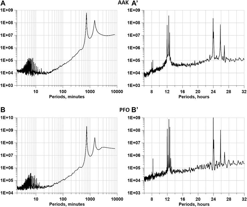
FIGURE 1. Power spectra estimates for 2 seismic stations: AAK ((a) and (a′) - Ala Archa, Kyrgyzstan, Latitude = 42.639, Longitude = 74.494) and PFO ((b) and (b′) - Pinon Flat, California, USA, Latitude = 33.611, Longitude = −116.456). Plots (a) and (b) correspond to range of periods from 2 up to 10000 minutes, whereas (b) and (b′) - to range of periods from 6 up to 32 hours.

Let us consider an auxiliary network of 50 reference points, the positions of which will be determined using the hierarchical cluster analysis of the positions of 229 seismic stations by the “far neighbor” method. This method of cluster analysis has the ability to form compact clusters (Duda et al., 2000). The positions of both 229 seismic stations and 50 reference points are shown in Figure 2.

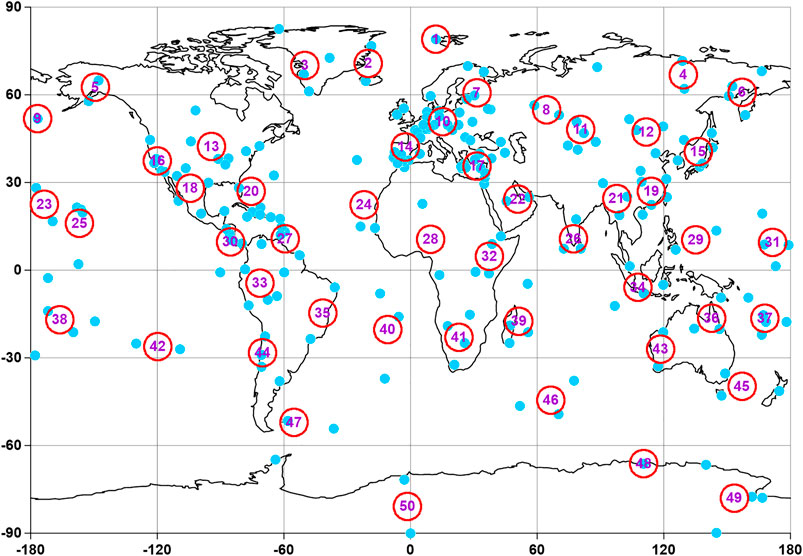
FIGURE 2. Blue circles - positions of 229 broadband seismic stations; red numbered circles - 50 reference points.

Minimum Wavelet-Based Normalized Entropy

Let $x\left(t\right)$ be the time series of a certain random signal, and let $t=1,\mathrm{.},N$ be the index enumerating the successive data points (the discrete time). Normalized entropy of the finite sample is defined by the following formula:

Here, $c_k,k=1,N$ are the coefficients of decomposition by certain orthogonal wavelet basis. We used 17 orthogonal Daubechies wavelets: 10 ordinary bases with minimal support width with 1–10 vanishing moments and seven bases of the so-called Daubechies symlets (Mallat, 1999) with 4–10 vanishing moments. We defined an optimal basis providing minimum to entropy in Eq. 1.

It should be noted that the sum of squared coefficients is equal to the variance (energy) of the signal $x\left(t\right)$. It means that quantity in Eq. 1 presents the entropy of energy distribution of the oscillations on the different frequencies and time scales.

The minimum normalized entropy $E_n$ was suggested in (Lyubushin, 2012) and was used for investigating seismic noise properties in (Lyubushin, 2013; Lyubushin, 2014; Lyubushin 2020a; Lyubushin 2020b; Lyubushin 2020c). The used entropy in Eq. 1 could be considered as multiscale and has some common features with entropy which was introduced in (Costa et al., 2003; Costa et al., 2005) for analysis of time series. The multiscale property follows from the use of orthogonal wavelet transform of the signal which allows decomposition into discrete dyadic time-frequency “atoms” with energy equal to $c_k^2$. In the natural time approach (Varotsos et al., 2011; Sarlis et al., 2018), the related entropy construction was proposed for data analysis. Application of Tsallis non-extensive entropy to investigating properties of ambient seismic noise was performed in (Koutalonis and Vallianatos, 2017; Vallianatos et al., 2019).

Our choice of wavelet-based entropy in Eq. 1 is due to the fact that it has the property to take into account the variety of vibration energy distribution over a system of independent time-frequency scale atoms, due to the use of a discrete orthogonal basis of functions with a finite support. In addition, the value in Eq. 1 is very simple and fast to calculate (because of using fast discrete wavelet transform), which is important when processing large amounts of data.

Figure 3 shows graphs of values of entropy at 50 reference points, calculated daily as medians of values at the five nearest operational stations. In order to get rid of the influence of tidal and thermal deformations of the Earth’s crust and to proceed to the study of noise characteristics, before calculating the normalized entropy in Eq. 1, an operation was performed to eliminate the trend by an 8th order polynomial within each daily time window. The values presented in Figure 3 can be considered as samples of typical entropy behavior in the vicinity of reference points, covering the entire world. These 50 time series with a sampling time step of 1 day, having 8,400 samples, will be the object of investigation further on in the article.

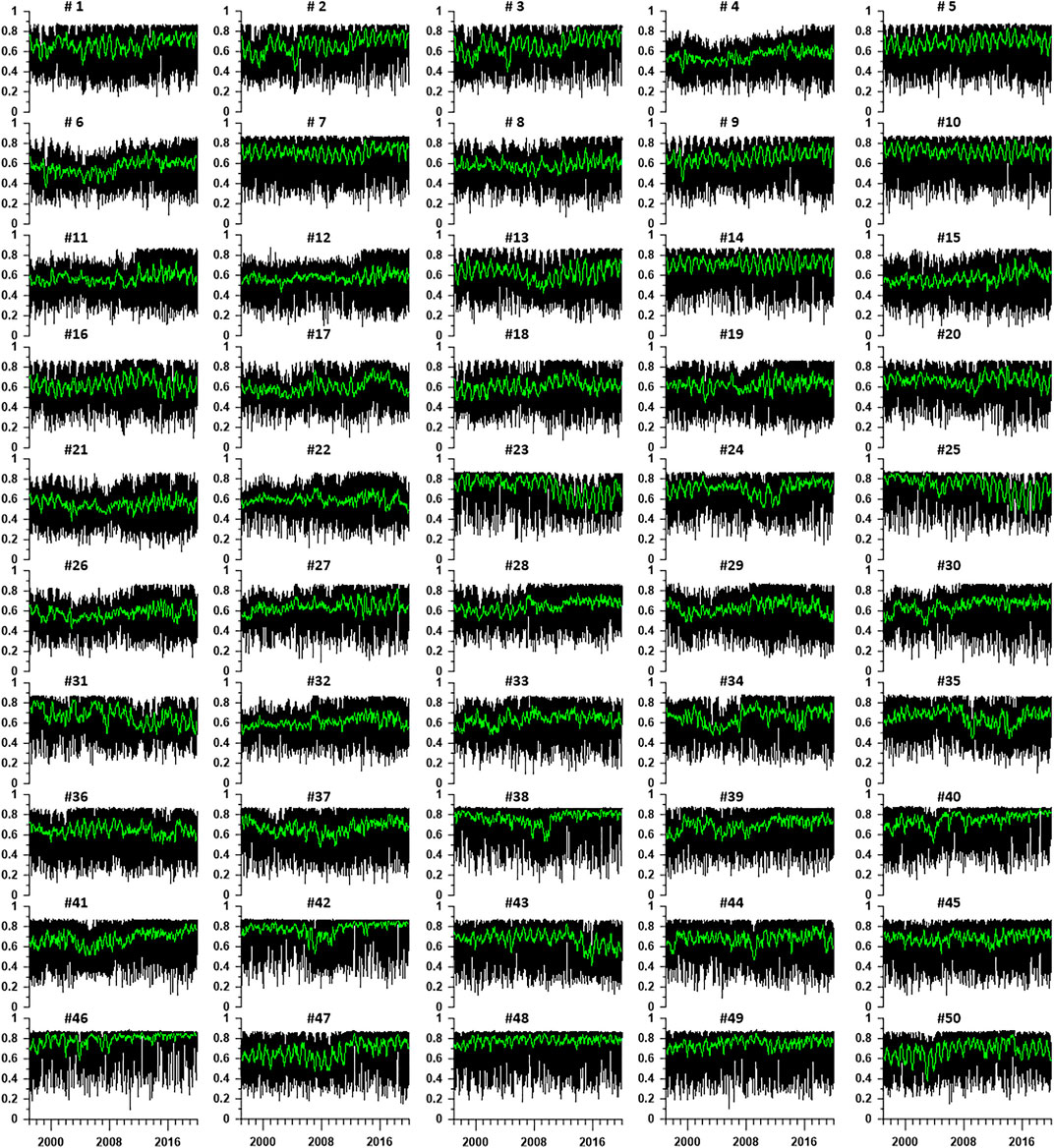
FIGURE 3. Graphs of daily values of the minimum normalized seismic noise entropy for each of the 50 reference points. The values are obtained as median values from the five nearest operational stations. The green lines represent the moving averages in a 57-day window.

Spatial Correlations of Entropy

Let us consider a sequence of time windows of 365 days in length taken with an offset of 3 days. In each such window, we calculate the correlation coefficients between the entropy values in all pairs of reference points (for 50 points, the number of such pairs is 1,225) and take the average value of their modules. In addition, we will separately consider strong correlations, the values of which exceed the threshold of 0.7.

Figure 4 shows the results of estimates of the temporal and spatial correlations of the entropy values at the reference points, obtained in a moving time window of 365 days in length, taken with a mutual shift of 3 days. The graphs are plotted depending on the position of the right end of the time window. Figure 4A represents the average values of all pairwise correlation coefficients, and Figure 4B represents maximum values of the correlation coefficient in each window. Figure 4C represents a graph of the number of strong pairwise correlations between entropy values at 50 reference points exceeding the 0.7 threshold. Figure 4D shows the maximum distances between pairs of reference points that have strong correlations.

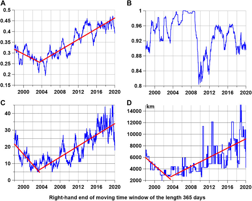
FIGURE 4. (A,B) Mean and maximum values of pairwise correlation coefficients of entropy values at 50 reference points. (C) The number of pairs of 50 reference points, between which in the current time window, there is a correlation exceeding the threshold of 0.7 in absolute value. (D) The maximum distance between pairs of reference points, between which a correlation has arisen in the current time window, exceeding the threshold of 0.7 in magnitude. The red lines represent piecewise linear trends with a corner point in 2003.5.

First of all, a common feature of the graphs in Figures 4A,C,D could be noticed, the presence of a time point 2003.5 of the position of the right end of the time window, for which the downward linear trend is abruptly replaced by an upward one and its growth continues until the end of 2019. This feature is highlighted in Figure 4 by graphs of piecewise linear trends depicted by red lines. Taking into account that the window length is 365 days, this means that the temporal and spatial dynamics of the global seismic noise entropy underwent rapid changes during the year time interval from mid-2002 to mid-2003. For the average value of the correlations (Figure 4A), this feature was previously identified in (Lyubushin, 2020a), where it was associated with the peculiarities of the uneven rotation of the Earth. The rapid increase in the number of strong correlations and their spatial scale since 2004, as seen in Figures 4C,D, is a new result.

Also, note the unusual behavior of the maximum correlation coefficient in Figure 4B—a sharp drop for the timestamp of the right end of the window at the end of 2009. After this drop, outliers began in the values of the maximum distances between the reference points with strong entropy correlations (Figure 4D).

Figure 5 shows the results of identifying strong correlations between the control points. In each 365-day time window, we connect with a straight line those pairs of reference points for which the calculated correlation coefficient in absolute value exceeded the threshold of 0.7. Figure 5A presents correlation connectivity for a time window with low number of strong correlations (2003 years, 10 correlations), whereas Figure 5A′ corresponds to the time window with a large number of strong correlations (from mid-2018 to mid-2019, 43 correlations). The whole number of time windows of 365 days in length taken with a mutual shift of 3 days within 23 years of observations (1997–2019) equals 2,679. Figure 5B presents a histogram with 100 bins for the set of distances between reference points with strong entropy correlations for all time windows. This histogram has three intervals of maximum: 1,250–1,400 km, 1,810–1,950 km, and 2,790–2,630 km. A question arises whether these most frequent intervals of strong correlation distances could occur because they are most frequent for the nearest distances between reference points. The whole number of nearest distances between reference points equals 37 varying from 1,111 km up to 4,880 km. Figure 5B′ presents histogram with 12 bins for this set of nearest distances. The histogram in Figure 5B′ has two intervals of maximum with distances 2,054–2,368 km and 2,682–2,996 km. Taking into account the roughness of the histogram in Figure 5B′, we can propose that maximum in a histogram of strong correlation distances could occur due to most frequent nearest distances between reference points. After comparing histograms in Figure 5B,B′ we can conclude that strong correlation distances which exceed 4,000 km reflect important changes in the global seismic noise spatial structure which could be connected with activation of global seismic process after 2004. These changes are illustrated by a broken linear trend in Figure 4D.

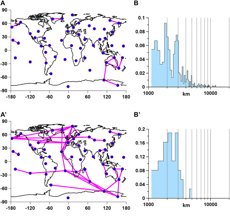
FIGURE 5. (A,A') Red lines show pairs of reference points, between which correlations of seismic noise entropy values that exceed the threshold of 0.7 arose in two time windows of 365 days in length with a small [(A), 2003-10 correlations] and a large number of strong correlations [(A'), 2018.5–2019.5-43 correlations]. (B) Histogram of distances between pairs of reference points, between which a correlation arose exceeding the threshold of 0.7, for all time windows of 365 days in length, taken with an offset of 3 days. (B') A histogram of the values of the nearest distances between all pairs of reference points.

Temporal dynamics of strong correlations could be presented as the graphs of the number of strong correlations for each of the reference points that arose in all moving time windows. The graphs of these numbers are shown in Figure 6.

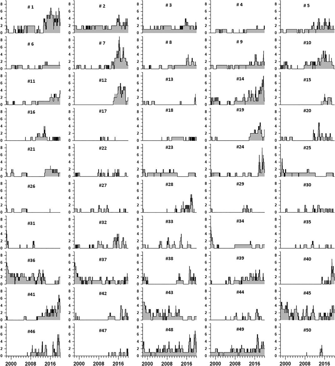
FIGURE 6. Graphs of the numbers of strong correlations that arose for each of 50 reference points with some other reference point in a sliding window of 365 days in length with an offset of 3 days. Graphs are plotted in dependence on position of the right end of the moving time window.

Figure 6 shows that the reference points differ greatly from each other in the number of strong correlations and in the time of their occurrence. Reference points with a large number of strong correlations can be called “sensitive” points on the Earth’s surface. It is interesting to represent graphically the distribution of the “intensity” of strong correlations and the change of this intensity over time in the form of maps. For each time window and for each reference point, you can specify the number of strong correlations, which, according to the graphs in Figure 6, can vary from 0 to 9. For each time window, we construct a spatial distribution map of the number of strong correlations by extrapolating the number of strong correlations from the reference points to the nodes with a regular grid of 100 nodes in longitude and 50 nodes in latitude using a Gaussian smoothing kernel (Duda et al., 2000):

Here ${\zeta }_k,k=1,\mathrm{.},m$, are the coordinates of reference points, in our case, $m=50$; are the number of strong correlations in the reference point #k, $r$ represents coordinates of nodes of regular grid, $d({\zeta }_k,r)$ is the distance from the surface of spherical Earth between points ${\zeta }_k$ and $r$, and $h$ is a smoothing parameter (bandwidth). We take the bandwidth $h={15}^{\circ }$ which corresponds to the distance ≈1,700 km from the surface of the spherical Earth. The value $\widehat{Z}\left(r\right)$ is extrapolated and the number of strong correlations from reference points to the nodes of regular grid is smoothed. We will call $\widehat{Z}\left(r\right)$ as the intensity of strong correlations for the node with coordinates $r$.

After calculating the values (Eq. 2) in all nodes of regular grid of the size for some time windows, we will have the map of correlation intensities corresponding to this window. Let us call such maps as “elementary” ones. For the sequence of time windows of the length 365 days taken with a mutual shift of 3 days covering interval 1997–2019, the number of elementary maps equals 2679. By averaging all elementary maps, we will have a mean map of strong correlation intensity which is presented in Figure 7A. According to this map, the most “sensitive” regions of the Earth are sub-Arctic including Greenland in the northern hemisphere and Australia and west Antarctica in the southern hemisphere. Equatorial latitudes and most of temperate latitudes are not “sensitive.”

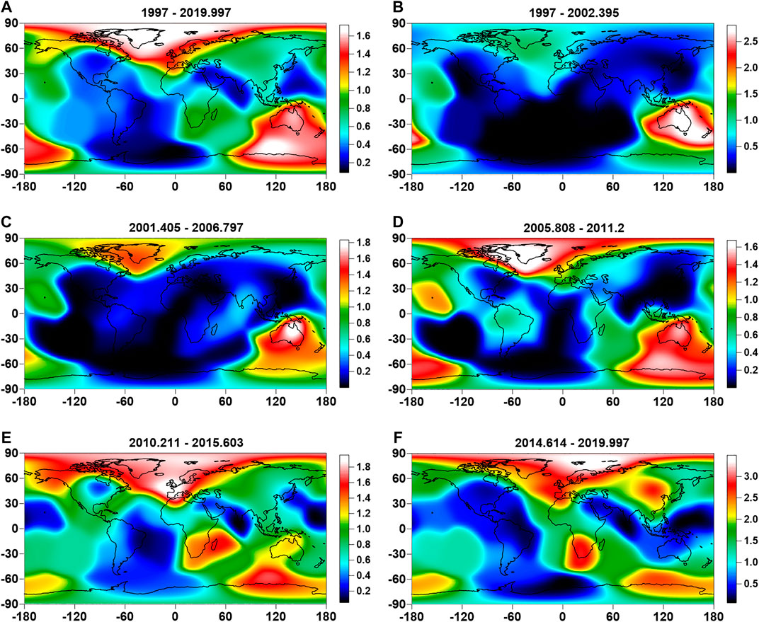
FIGURE 7. Averaged maps of intensity of correlation links which were obtained by spatial smoothing and extrapolating numbers of strong correlations within time windows of the length 365 days with a mutual shift of 3 days in 50 reference points (Figure 6) by using Gaussian kernel with smoothing radius 15°. Each map has time marks of most left and most right ends of time windows laying between two dates, given in fractional year format. Map (A) is obtained by averaging elementary maps from all time windows. Maps (B–F) correspond to averaging of equal successive number of elementary 365-day maps.

Other maps in Figure 7 present the temporal dynamics of correlation intensity as the sequence of maps which are obtained by averaging equal successive parts: 536 elementary maps in Figures 7B–E and 535 elementary maps in Figure 7F. From the sequence of maps in Figures 7B–F, it can be seen that the correlation intensity at the beginning of the considered time interval was maximum in the south, but then moved to the north.

Connection of Seismic Noise Entropy to Irregularity of Earth’s Rotation

The influence of the irregularity of the Earth’s rotation on the sequence of strong earthquakes has been studied in many works, for example, in (Shanker et al., 2001; Bendick and Bilham, 2017). This article continues the study of the relationship between the irregularity of rotation with the synchronization of the properties of seismic noise and the possible triggering effect of the irregular rotation of the planet on the seismic process, begun in (Lyubushin, 2020a; Lyubushin, 2020b).

Figures 8A,B present graphs of LOD) and mean noise entropy which is obtained by averaging all values from reference points (Figure 3). The data on the length of the day are taken from the International Earth Rotation and Reference Systems Service (IERS) database from the address https://hpiers.obspm.fr/iers/eop/eopc04/eopc04.62-now.

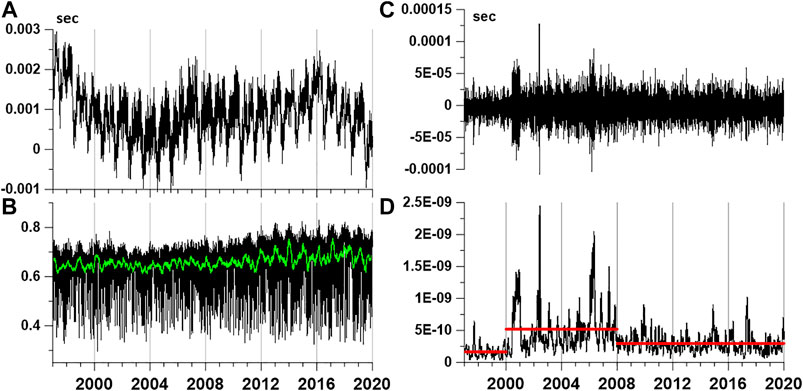
FIGURE 8. (A) Values of the length of the day [time series length of day (LOD)]. (B) Mean values of the minimum normalized seismic noise entropy for all 50 control points in Figure 3; green line presents the moving average in a 57-day window. (C) High-frequency component of LOD with periods less than 6 days. (D) Variance of high-frequency LOD component within a moving time window of 28 days in length; red lines present mean values of variance in three successive time fragments: 1997–2000.106, 2000.106–2007.926, and 2007.926–2020.

Figure 8C is a graph of high-frequency LOD component with periods less than 6 days, and Figure 8D presents an estimate of variance of high-frequency LOD variations within moving time window of the length 28 days. We can notice that evolution of high-frequency LOD component variance could be split into three time intervals, 1997–2000.106, 2000.106–2007.926, and 2007.926–2020, with different mean values which are drawn by horizontal red lines. Bounds of three time intervals in fractional years were found automatically from minimum of variance of deflections from local mean values. The time interval 2000.106–2007.926 corresponds to high power of high-frequency LOD variations. This time interval is interpreted as the reason of abrupt changes in temporal and spatial correlations of global seismic noise properties which are presented in Figure 4 (Lyubushin, 2020a; Lyubushin, 2020b).

Figure 9A shows the graphs of the logarithm of energy (Joules) released as a result of seismic events in the whole world in a moving time window of length 365 days with a 3-day shift, whereas Figure 9B is the parallel graph of bursts maxima of squared coherence between LOD and daily mean entropy in the same time windows. Information about global seismicity is taken from the USGS site from the address https://earthquake.usgs.gov/earthquakes/search/. The coherence estimation was performed using a 5th-order vector autoregressive model (Marple, 1987) with preliminary removal of linear trends and transition to increments. Figure 9C presents the time-frequency diagram of squared coherence evolution, and we can notice that bursts of coherence are mainly concentrated within narrow frequency band with periods from 11 up to 14 days. Estimates of maxima of squared coherence were already used in (Lyubushin, 2020a; Lyubushin, 2020b) when analyzing trends in the properties of global seismic noise and their relationships with the uneven rotation of the Earth.

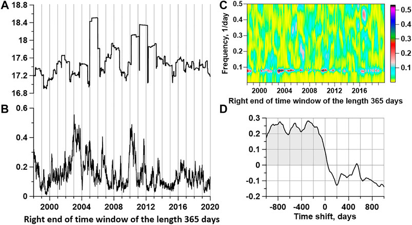
FIGURE 9. (A) A plot of the decimal logarithm of the released seismic energy (Joules) in a sliding time window of 365 days. (B) The maximum values with respect to the frequencies of the quadratic coherence between length of day (LOD) and the average value of the entropy in a moving time window of 365 days. (C) A time-frequency diagram of the change in the quadratic coherence between the LOD time series and the average entropy value (see panel 8B) in a sliding window of 365 days long with an offset of 3 days. (D) The correlation function between the values of the logarithm of the released seismic energy and the maximum of coherence between the day length and the average value of entropy. Negative values of time shifts correspond to the lag in the release of seismic energy relative to bursts of coherence between LOD and noise entropy.

From Figures 9A,B, it is visually noticeable that the curve of the logarithm of the released energy often lags after the curve of the maxima of the coherence spectrum when it is calculated in a moving time window.

Let us quantitatively estimate this shift by calculating their cross-correlation function for time shifts ± 1,000 days, the graph of which is shown in Figure 9D. From the estimate of the correlation function in Figure 9D, it can be seen that its values for negative time shifts significantly exceed the values for positive shifts, which confirms the fact that the release of seismic energy is delayed, relative to bursts of the coherence measure. As for the lag time, it is not determined unambiguously, since the values of the correlation function for negative shifts actually reach a certain plateau, which contains three local maximums for shifts of -280, -510, and -720 days.

The estimation of the coherence maxima between LOD and average entropy in a 4-year window deserves special attention. Since 1 year out of four consecutive years is a leap year, the length of the 4-year time window is 1,461 days. Figure 10 shows a graph of estimates of the maxima of the quadratic coherence in a sliding time window with a length of 1,461 days with an offset of 3 days. Since the window length is four times larger than the previously used 365-day window, a model of the order 20 was used to estimate the coherence spectrum instead of the 5th-order autoregressive model.

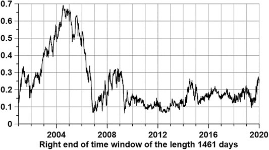
FIGURE 10. Maximum values of the quadratic coherence between length of day and the average value of the entropy in a moving time window of 1,461 days (4 years).

The coherence estimate in Figure 10 is interesting because before the Sumatran mega-earthquake at the end of 2004, after which the global seismic process began to activate, the coherence estimate reaches a very significant maximum, reaching almost 0.7. We interpret this peak of coherence as a manifestation of the triggering effect of the anomaly of the uneven rotation of the Earth, previously considered in (Lyubushin, 2020a; Lyubushin, 2020b).

Conclusion

Software tools have been developed to study the global low-frequency seismic noise recorded continuously from the beginning of 1997 to the end of 2019 on a network of 229 broadband seismic stations located around the world. The analyzed value is determined daily at the nodes of the auxiliary network of 50 reference points as the median of the Shannon information entropy of the distribution of the squares of the orthogonal wavelet coefficients of the seismic noise waveforms at the five nearest operable stations. The time interval from mid-2002 to mid-2003 was determined, when the downward trend of the average correlation of the noise entropy changed abruptly to an upward trend, which persists until the end of 2019. Along with the growth of the average correlation, an increase in the radius of spatial correlations of the noise entropy is observed, and the increasing trend of spatial correlations persists until the end of 2019 as well.

At the same time, with an increase in the average correlation, an increase in the radius of spatial correlations of the entropy of noise is observed, and after 2010, bursts of maximum distances between the reference points with strong pairwise entropy correlations, reaching 10–15 thousand km, began to appear.

These features of the behavior of global seismic noise are interpreted as a result of the triggering effect of the unevenness of the Earth’s rotation on an increase in noise correlation and, at the same time, on an increase in the intensity of the strongest seismic events in the world after the Sumatran mega-earthquake of December 26, 2004, M = 9.3. This interpretation is confirmed by a correlation estimate of the seismic energy release lag in relation to bursts of coherence between the average entropy value and the length of the day when estimated in a sliding time window of 365 days.

The emergence of sharp bursts of an increase in the maximum distance between the reference points with a strong entropy correlation after 2010 can be associated with the destabilization of the global seismic noise field after two mega-earthquakes close in time: February 27, 2010, M = 8.8, in Chile and March 11, 2011, M = 9.1, in Japan. The persistence of an increasing trend of increasing average correlations of noise entropy and distances at which maximum correlations occur is interpreted as persistence of a high global seismic hazard that arose after 2004. A spatial measure of entropy correlations was introduced by extrapolating and averaging the numbers of strong correlations at each reference point in an annual sliding time window using a Gaussian smoothing kernel function. It turned out that areas of strong correlation are adjacent to the polar regions of the Earth, and for the period 1997–2019, the region of strong entropy correlation gradually moved from the south to the north.

Data Availability Statement

Publicly available datasets were analyzed in this study. These data can be found as follows: http://www.iris.edu/mda/_GSN, http://www.iris.edu/mda/G, http://www.iris.edu/mda/GE, https://hpiers.obspm.fr/iers/eop/eopc04/eopc04.62-now, https://earthquake.usgs.gov/earthquakes/search/.

Author Contributions

The author is the developer and programmer of all algorithms used in the article.

Conflict of Interest

The authors declare that the research was conducted in the absence of any commercial or financial relationships that could be construed as a potential conflict of interest.

Funding

The research was supported by the Russian Foundation for Basic Research, Grant No. 18-05-00133, project “Estimation of fluctuations of seismic hazard on the basis of complex analysis of the Earth’s ambient noise.”

References

Ardhuin, F., Stutzmann, E., Schimmel, M., and Mangeney, A. (2011). Ocean wave sources of seismic noise. J. Geophys. Res. 116, C09004. doi:10.1029/2011jc006952
Aster, R. C., McNamara, D. E., and Bromirski, P. D. (2008). Multidecadal climate-induced variability in microseisms. Seismol Res. Lett. 79, 194–202. doi:10.1785/gssrl.79.2.194
Bendick, R., and Bilham, R. (2017). Do weak global stresses synchronize earthquakes?. Geophys. Res. Lett. 44, 8320–8327. doi:10.1002/2017GL074934
Berger, J., Davis, P., and Ekström, G. (2004). Ambient earth noise: a survey of the global seismographic network. J. Geophys. Res. 109, B11307. doi:10.1029/2004jb003408
Costa, M., Goldberger, A. L., and Peng, C.-K. (2005). Multiscale entropy analysis of biological signals. Phys. Rev. E 71 021906. doi:10.1103/physreve.71.021906
Costa, M., Peng, C.-K., Goldberger, A. L., and Hausdorff, J. M. (2003). Multiscale entropy analysis of human gait dynamics. Physica A 330, 53–60. doi:10.1016/j.physa.2003.08.022
Duda, R. O., Hart, P. E., and Stork, D. G. (2000). Pattern classification. New York, Chichester, Brisbane, Singapore, Toronto: Wiley-Interscience Publication
Friedrich, A., Krüger, F., and Klinge, K. (1998). Ocean-generated microseismic noise located with the Gräfenberg array. J. Seismol. 2 (1), 47–64. doi:10.1023/a:1009788904007
Fukao, Y., Nishida, K., and Kobayashi, N. (2010). Seafloor topography, ocean infragravity waves, and background love and rayleigh waves. J. Geophys. Res. 115, B04302. doi:10.1029/2009jb006678
Grevemeyer, I., Herber, R., and Essen, H.-H. (2000). Microseismological evidence for a changing wave climate in the northeast Atlantic Ocean. Nature 408, 349–352. doi:10.1038/35042558
Kobayashi, N., and Nishida, K. (1998). Continuous excitation of planetary free oscillations by atmospheric disturbances. Nature 395, 357–360. doi:10.1038/26427
Koper, K. D., and de Foy, B. (2008). Seasonal anisotropy in short-period seismic noise recorded in South Asia. Bull. Seismol. Soc. Am. 98, 3033–3045. doi:10.1785/0120080082
Koper, K. D., Seats, K., and Benz, H. (2010). On the composition of Earth’s short-period seismic noise field. Bull. Seismol. Soc. Am. 100 (2), 606–617. doi:10.1785/0120090120
Koutalonis, I., and Vallianatos, F. (2017). Evidence of non-extensivity in earth’s ambient noise. Pure Appl. Geophys. 174, 4369–4378. doi:10.1007/s00024s-017-1669-9
Lyubushin, A. (2012). Prognostic properties of low-frequency seismic noise. Nat. Sci. 4, 659–666. doi:10.4236/ns.2012.428087
Lyubushin, A. (2013). How soon would the next mega-earthquake occur in Japan? Nat. Sci. 5, 1–7. doi:10.4236/ns.2013.58A1001
Lyubushin, A. (2018). “Synchronization of geophysical fields fluctuations -,” in Complexity of seismic time series: measurement and applications. Editors T. Chelidze, L. Telesca, and F. Vallianatos, (Amsterdam, Oxford, Cambridge: Elsevier 2018), Chap. 6, 161–197.
Lyubushin, A. (2020a). Trends of global seismic noise properties in connection to irregularity of Earth’s rotation. Pure Appl. Geophys. 177 (2), 621–636. doi:10.1007/s00024-019-02331-z
Lyubushin, A. A. (2014). Analysis of coherence in global seismic noise for 1997–2012. Izvestiya Phys. Solid Earth. 50 (3), 325–333. doi:10.1134/s1069351314030069
Lyubushin, A. A. (2015). Wavelet-based coherence measures of global seismic noise properties. J. Seismol. 19 (2), 329–340. doi:10.1007/s10950-014-9468-6
Lyubushin, A. A. (2017). Long-range coherence between seismic noise properties in Japan and California before and after Tohoku mega-earthquake. Acta Geod. Geophys. 52, 467–478. doi:10.1007/s40328-016-0181-5
Lyubushin, A. A. (2020c). Seismic noise wavelet-based entropy in southern California. J. Seismol. doi:10.1007/s10950-020-09950-3
Lyubushin, A. (2020b). Connection of seismic noise properties in Japan and California with irregularity of Earth’s rotation. Pure Appl. Geophys. 177, 4677–4689. 10.1007/s00024-020-02526-9
Mallat, S. A. (1999). Wavelet tour of signal processing. 2nd Edn. San Diego, London, Boston, New York, Sydney, Tokyo, Toronto: Academic Press
Marple, S. L., and Jr, (1987). Digital spectral analysis with applications. Englewood Cliffs, NJ: Prentice‐Hall, Inc.
Nishida, K., Kawakatsu, H., Fukao, Y., and Obara, K. (2008). Background love and rayleigh waves simultaneously generated at the Pacific Ocean floors. Geophys. Res. Lett. 35, L16307. doi:10.1029/2008gl034753
Nishida, K., Montagner, J.-P., and Kawakatsu, H. (2009). Global surface wave tomography using seismic hum. Science 326 (5949), 112. doi:10.1126/science.1176389
Rhie, J., and Romanowicz, B. (2004). Excitation of Earth’s continuous free oscillations by atmosphere-ocean-seafloor coupling. Nature 431, 552–554. doi:10.1038/nature02942
Rhie, J., and Romanowicz, B. (2006). A study of the relation between ocean storms and the Earth’s hum. Geochem. Geophys. Geosyst. 7 (10). doi:10.1029/2006gc001274
Sarlis, N. V., Skordas, E. S., Mintzelas, A., and Papadopoulou, K. A. (2018). Micro-scale, mid-scale, and macro-scale in global seismicity identified by empirical mode decomposition and their multifractal characteristics. Sci. Rep. 8, 9206. doi:10.1038/s41598-018-27567-y
Shanker, D., Kapur, N., and Singh, V. P. (2001). On the spatio temporal distribution of global seismicity and rotation of the earth - a review. Acta Geod. Geophys. Hung. 36, 175. doi:10.1556/ageod.36.2001.2.5
Stehly, L., Campillo, M., and Shapiro, N. M. (2006). A study of the seismic noise from its long-range correlation properties. J. Geophys. Res. 111, B10306. doi:10.1029/2005jb004237
Tanimoto, T. (2001). Continuous free oscillations: atmosphere-solid earth coupling. Annu. Rev. Earth Planet. Sci. 29, 563–584. doi:10.1146/annurev.earth.29.1.563
Tanimoto, T. (2005). The oceanic excitation hypothesis for the continuous oscillations of the Earth. Geophys. J. Int. 160, 276–288. doi:10.1111/j.1365-246X.2004.02484.x
Vallianatos, F., Koutalonis, I., and Chatzopoulos, G. (2019). Evidence of Tsallis entropy signature on medicane induced ambient seismic signals. Physica A 520, 35–43. doi:10.1016/j.physa.2018.12.045
Keywords: entropy, seismic noise, correlation, length of day, wavelets, coherence
Citation: Lyubushin A (2020) Global Seismic Noise Entropy. Front. Earth Sci. 8:611663. doi: 10.3389/feart.2020.611663
Received: 29 September 2020; Accepted: 27 October 2020;
Published: 24 November 2020.
Edited by:
Giovanni Martinelli, National Institute of Geophysics and Volcanology, ItalyReviewed by:
Filippos Vallianatos, Technological Educational Institute of Crete, GreecePaolo Harabaglia, University of Basilicata, Italy
Copyright © 2020 Lyubushin. This is an open-access article distributed under the terms of the Creative Commons Attribution License (CC BY). The use, distribution or reproduction in other forums is permitted, provided the original author(s) and the copyright owner(s) are credited and that the original publication in this journal is cited, in accordance with accepted academic practice. No use, distribution or reproduction is permitted which does not comply with these terms.
*Correspondence: Alexey Lyubushin, lyubushin@yandex.ru