An Intelligent Radiomic Approach for Lung Cancer Screening

Abstract

The efficiency of lung cancer screening for reducing mortality is hindered by the high rate of false positives. Artificial intelligence applied to radiomics could help to early discard benign cases from the analysis of CT scans. The available amount of data and the fact that benign cases are a minority, constitutes a main challenge for the successful use of state of the art methods (like deep learning), which can be biased, over-fitted and lack of clinical reproducibility. We present an hybrid approach combining the potential of radiomic features to characterize nodules in CT scans and the generalization of the feed forward networks. In order to obtain maximal reproducibility with minimal training data, we propose an embedding of nodules based on the statistical significance of radiomic features for malignancy detection. This representation space of lesions is the input to a feed forward network, which architecture and hyperparameters are optimized using own-defined metrics of the diagnostic power of the whole system. Results of the best model on an independent set of patients achieve 100% of sensitivity and 83% of specificity (AUC = 0.94) for malignancy detection.

1. Introduction

Lung cancer is both the most frequently diagnosed cancer and cause of cancer death [1]. The National Lung Screening Trial (NLST) (Study performed in United States) [2] and Dutch-Belgian Randomized Lung Cancer Screening Trial (NELSON) [3] have shown that lung cancer screening (LCS) with computed tomography of low dose (CTLD) reduces mortality by 20–25%. However, the average of false positive rate of the radiological diagnosis obtained by visual inspection of scans was 23% of the nodules detected. This inaccuracy meant long follow-up of patients with repetitive CT or performing an invasive procedure like a biopsy or surgery, which accounted to be futile in 73% of the cases. A reduction of false positives would increase the efficiency of screening for early detection of lung cancer.

The largest screening program in Europe, the NELSON study, introduced volumetry of the nodules in consecutive CT, which meant a significant reduction of the average of false positive rate to 13%. This suggests that the application of radiomics [4] (a recent discipline that extracts a large number of image features correlating to treatment outcome), could represent a critical shift in the reduction of the false positive rate and an improvement of early diagnosis of lung cancer.

In this sense, in a pilot study [2] the authors retrospectively extracted 150 quantitative image features and performed a random forest classification, which finally obtained a significantly better predictive value than volumetry alone (AUC = 0.87 vs. 0.74). More recently, Peikert et al. [5] built a radiomic classifier based upon eight quantitative radiologic features selected by the least absolute shrinkage and selection operator (LASSO) method from 726 indeterminate nodules of the LCST. These eight features include variables capturing location, size, shape descriptors and texture analysis. In this retrospective study, the optimism-corrected AUC for these eight features was 0.939 with a sensitivity and specificity of, respectively, 90% and 85%.

An alternative to classic radiomics is the use of machine learning methods that extract image features using well known methods such as, Gabor, Local Binary Patterns (LBP), or SIFT descriptor to represent a nodule. Then machine learning technics (e.g., Support Vector Machine (SVM) and Random Forest) are used to define a classification of nodules in this representation space according to their diagnosis [6,7]. This methods achieve better diagnostic power than radiomic methods with AUC equal to 0.97, sensitivity equal to 96% with 95% of specificity for [6].

Recently, deep CNN (CNN stands for Convolutional Neural Network) have achieved great success in various computer vision tasks, such as image classification, segmentation, and enhancement. Researchers are therefore inspired to classify nodules by using CNNs. Existing works based on CNNs can be classified according to some key points: input data (2D or 3D), level of the input image (volume, slice, nodule), CNN architecture, resources needed and obtained performance.

The early work of Shen et al. proposed to use a multi-crop CNN [8] to make the model robust to scales of nodules while keeping 2D input images. Results showed an overall accuracy (including malign and benign cases) of 87%. However, the authors did not report sensitivity for malignancy detection and specificity for discarding benign nodules and, thus, its true clinical value is uncertain.

Since nodules are 3D structures, recent works have addressed the problem using 3D CNNs. Yan et al. [9] explored 3D CNNs for pulmonary nodule classification in comparison to a slice-level 2D CNN and a nodule-level 2D CNN analysis. The 3D approach was the best performer with a 87% of overall accuracy and similar specificity and sensitivity at the cost of a significantly higher demand of computational resources and annotated data. Zhu et al. [10] used 3D deep dual path networks (DPNs) a 3D Faster Regions with Convolutional Neural Net (R-CNN) designed for nodule detection with 3D dual path blocks and a U-net-like encoder-decoder structure to effectively learn nodule features. Despite the complex architecture used, this approach could only achieve a 81% of sensitivity and specificity was not reported. Jiang et al. [11] sequentially deployed a contextual attention module and a spatial attention module to 3D DPN to increase the representation ability. A main novelty of this work is that it ensembles different model variants to improve the prediction robustness. Results show an increase of sensitivity to 90% while keeping a specificity similar to [9]. A main concern is the huge amount of parameters that require extensive data and computational resources for training. In an attempt to minimize computational and data costs, the very recent [12] uses automatic Neural Architecture Search (NAS) technique [13] to design optimal 3D network architectures including attention modules. Results on a subset of the LIDC-IDRI database [14] show a specificity of 95% at the cost of a drop in sensitivity to 85%.

A main challenge in the application of deep learning to biomedical problems is the limited amount of good quality data with annotations, which is a must for training new models with complex architectures. Besides, in the case of benign nodule screening, this is aggravated with the fact that the problem is highly unbalanced with benign cases being the minority class. Under such experimental settings, models are often over-fitted [15] results are non-reproducible [15,16] and most times [9,10,11,12] do not outperform conventional machine learning approaches [6]. Another pitfall, especially for deep methods is models should also be easily interpreted from a clinical point of view to allow the analysis of the clinical factors that have an impact on the clinical decision [17].

The output of a classic CNN are features that have no meaning from radiological point of view. In this way, introducing classic radiomic features in the models will be helpful for radiologist in the interpretability of the results by means of most correlated features to malignancy of tumours. It is worth to mention that radiomic features can describe tumour heterogeneity [18], which is a parameter related to malignancy and well known from radiologist. To address the above challenges, we propose to embed 2D slices into a low dimensional radiomic space defined by the classic radiomic features that significantly correlate to malignancy. These features are the input to a fully connected network with an architecture optimized in order to ensure maximum clinical outcome. To do so, novel specific criteria and metrics measuring diagnostic power are presented. Models were optimized in a set of 51 nodules coming from an own collected data base. Results on an independent set of patients from the same data base and LIDC-IDRI database show that our approach outperforms deep approaches with only requiring 290 parameters (in contrast to the thousands required by deep methods).

2. Materials and Methods

This work complies with the fundamental ethical principles of research (Declaration of Helsinki—Fortaleza/Brazil, 2013). In each case, informed consent is requested, and both the images with clinical data are treated anonymously, safeguarding the confidentiality of the patient. This study was approved by the ethics committee of the HUGTiP prior to the start of recruitment (CEIC H. Germans Trias i Pujol: PI-19-169).

2.1. Dataset Description

The patients were recruited at the Germans Trias i Pujol University Hospital (HUGTiP), Barcelona, Spain, from which images and clinical/demographic data were collected between December 2019 and September 2020. The 60 recruited patients have CT-chest and pulmonary nodule (PN) tributary of surgery, and meet the following inclusion and exclusion criteria. The inclusion criteria includes: have a single PN, diameter from 8 to 30 mm, final diagnosis of non-small cell lung carcinoma and non-malignant tumor. And the exclusion criteria includes: have been previously diagnosed with lung cancer, diagnosis of uncured extra-pulmonary cancer (except non-melanoma skin cancer), pregnancy, have received chemotherapy or cytotoxic drugs in the last 6 months and decline to sign the consent. The PNs have been classified in every case by means of a biopsy.

Scans were acquired with GE Medical Systems and Philips CT scan. For both devices, acquisition parameters in all cases were 120 kv, 100–350 mA (dose modulation range), soft tissue reconstructions, high frequency algorithms and 512 × 512 matrix. These parameters are the gold standard used to ensure enough scan resolution and quality to radiologically evaluate malignancy [19,20].

Table 1. Details of the acquisition parameters by scanner manufacturer.

Description\Manufacturer	GE Medical Systems	Philips
Model Name	LightSpeed VCT BrightSpeed Optima CT540 Discovery ST	GeminiGXL 16 Brilliance 16 TruFlight Select
Convoluton Kernel	SOFT STANDARD LUNG	B YA YB YC
Pixel XY size	0.56–0.87	0.36–0.72
Slice Thickness	0.63–1.25	1–2
Benign Nodules	3	6
Malignant Nodules	21	30

report the acquisition setting for each manufacturer, as well as the number of benign and malign nodules.

A respiratory medicine physician with seven years of experience annotated the Region of Interest (ROI) of each nodule with 3D-Slicer (version 4.11.20200930), which is a free, open source and multi-platform software package widely used for medical, biomedical, and related imaging research. The physician was asked to define ROIs fitting the minimal nodule space as possible. The coordinates of the bounding box defining the ROI were stored in csv format for its further use in the method pre-processing step described in Section 2.3. A ROI per patient was annotated, since the cases conforming our database have one nodule per patient. The

Table 2. Details of our database.

	Description	Male	Female	Total
Demographic population	Patients Age avg ± std Benign PNs Malign PNs	36 70.67 ± 6.87 5 31	24 63.96 ± 12.35 4 20	60 67.98 ± 9.92 9 51
Nodule characterization	Benign Slices min/max/avg Malign Slices min/max/avg	6/111/48 8/152/45	28/39/32 12/82/45	6/111/41 8/152/43

shows detailed information about our database. We report demographic information, as well as, the minimum, maximum and every number of slices for each nodule type and sex.

2.2. Methodology Description

Our methodology aggregates, for each nodule, the classification at slice level to obtain a prediction of nodule malignancy. The classification of 2D slices bases on radiomic 2D textural features computed on a mask of the nodule to implicitly account for (2D) shape. Texture descriptors are the input to a feedforward neural network with optimized architecture.

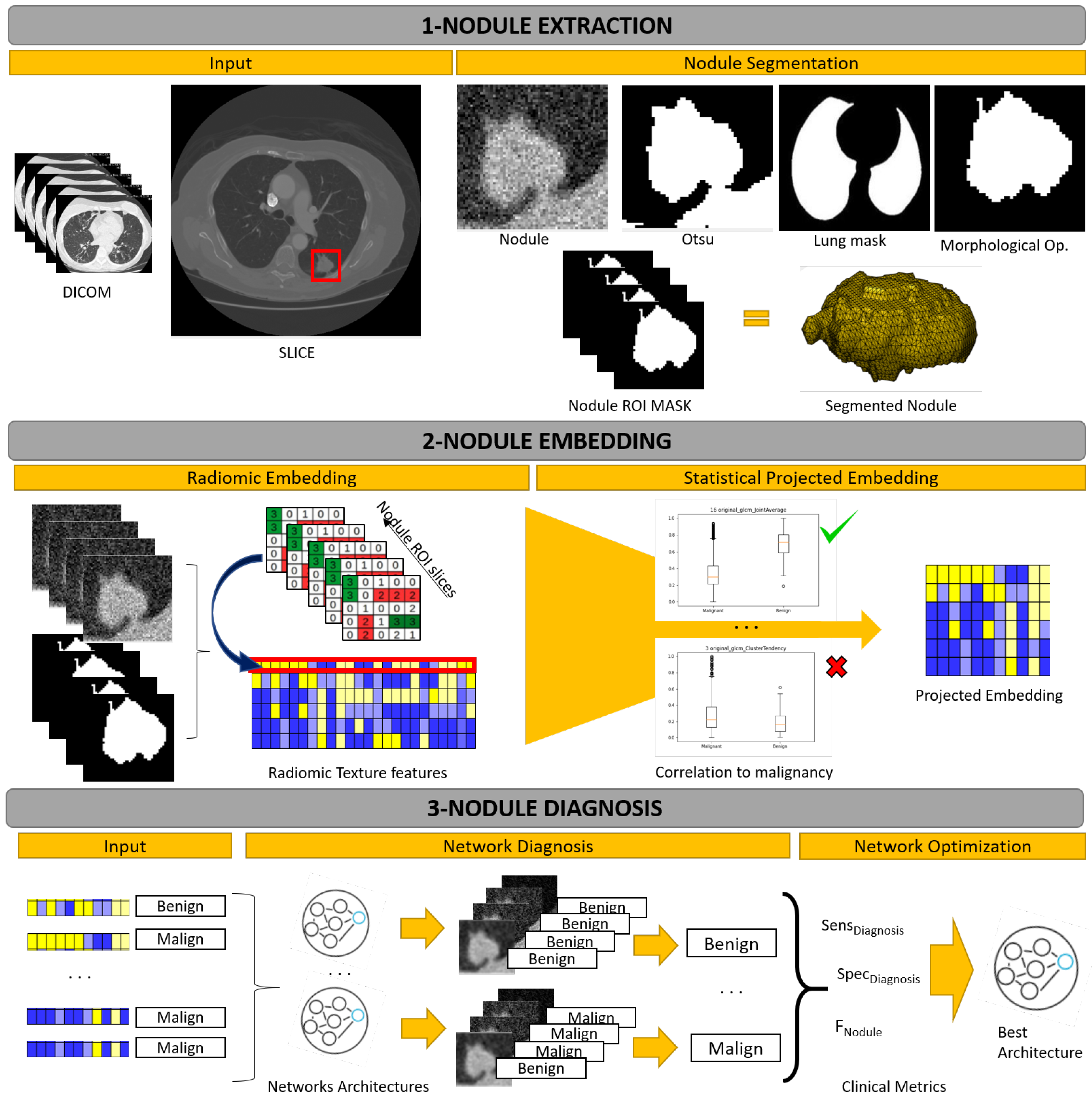
Figure 1 shows a general overview of our workflow, which consists in 3 main phases: extraction of nodules from CT scans, embedding of nodules into a space representing malignancy and nodule diagnosis with optimized network architecture. In the extraction step, the nodule is segmented in the ROI volumes using Otsu thresholding and morphological operations. In the embedding phase, PyRadiomics [21] GLCM descriptors are computed in 2D slices of masked volumes and a t-test is used to select those features that significantly correlate to malignancy. In the diagnosis phase, the selected features are the input to an optimized feedforward network trained and the most frequent classification among each nodule 2D slices determines the final diagnosis. The architecture and hyperparameters of the diagnostic networks are optimized according to an own-defined metrics measuring the clinical performance of the system.

2.3. Nodule Extraction

In the preprocessing phase we used the anonymized CT-chest DICOMs and the annotated nodule ROIs. A nodule ROI always includes the intranodule region (inside nodule region), but depending on the nodule shape, the perinodular region (around nodule region) is included in greater or lesser extent. Since, in [22,23], it is reported that the importance of using perinodular region in the classification of benign and malignant nodules, the size of ROIs was enlarged 15% of its original size. The volume ROI extracted using the coordinates of the annotated bounding box is the input to the whole workflow. This is the only manual annotation required.

In order to segment the nodule, we applied Otsu thresholding to the ROI volume. Since the segmentation of peripheral nodules can include non-pulmonary tissue, the binarized volumes were masked with a segmentation of lungs. The final nodule segmentation was the largest connected component of the masked volumes. The segmentation of lungs was computed using thresholding and morphological operations [24]. Specifically, CT lungs were selected as the larger connected component of the voxels with intensity between 950 to −300 Hounsfield Units, followed by a closing with a structuring element of size 5.

2.4. Nodule Embedding

To extract radiomics features we used PyRadiomics [21] (version 3.01), an open-source python package for the extraction of radiomic features from medical imaging volumes. PyRadiomics features include shape features, first order features, and textural features (Gray Level Co-ocurrence Matrix (GLCM), Gray Level Size Zone (GLSZM), Gray Level Run Length Matrix (GLRLM) and Gray Level Dependency Matrix (GLDM)) describing several aspects of the lesion. In this study, we used GLCM texture features [25] by its proven efficiency for cancer diagnosis in a wide range of medical imaging modalities [26,27,28,29,30].

GLCM textural features are probabilistic descriptors computed from a gray level co-ocurrence matrix. This matrix encodes textural patterns in a neighbourhood of each pixel based on different contrasts. To do so, intensity gray values are first discretized using the histogram of the original volume intensity. The width of the histogram bins sets the granularity that GLCM features describe, since neighbouring pixels with a difference in gray level below such parameter are filtered. Bin width, namely Δ, is given by:

$$\Delta =\frac{max(Pixel\_value)-min(Pixel\_value)}{Nbins}$$

(1)

for $Pixel\_value$ the intensities of the volume and $Nbins$ the number of histogram bins.

In [29,30], the authors showed the importance of, both, intensity ranges and number of bins. It is reported that a fixed bin count between 30 and 130 bins has good reproducibility and performance. In order to allow for different ranges of intensity in ROIs, while still keeping the texture features informative and comparable inter lesion [26], we first normalize the CT Hounsfield Units (HU) to a common intensity range. Hounsfield Units are related to intensity values with the following linear transformation:

$$HU=Pixel\_value\ast Slope+Intercept$$

(2)

for $Slope$ and $Intercept$ are acquisition parameters of the CT scan.

HU were mapped to a common intensity range $[0,MaxIntensity]$ using the following formula:

$$\begin{array}{c}\hfill Pixel\_value=\frac{(HU-Intercept)/Slope}{max\left(HU\right)-min\left(HU\right)}\ast MaxIntensity\end{array}$$

(3)

$$\begin{array}{c}\hfill =\frac{(HU-Intercept)/Slope}{4000}\ast MaxIntensity\end{array}$$

(4)

where $max\left(HU\right)=2976$ was computed as the maximum of the training set volumes HU and $min\left(HU\right)=-1024$ is the HU value for air. The intensity range $MaxIntensity$ and number of bins, $Nbins\in [30,130]$, are hyper-parameters that were set using grid-search. The optimal values were $MaxIntensity=24$ and $Nbins=128$.

The GLCM features (extracted on 2D slices) are selected according to their correlation to lesion malignancy. It is expected that the most discriminant features have values significantly different for slices containing malign and benign nodules. Such differences are detected, for each GLCM feature, with a Student t-test comparing average values for malign and benign slices. In order to account for unbalancing between malignant and benign cases, a k-fold subsampling of malignant slices was performed and max-voting aggregation of significance was used to select the most discriminative features. Sample size was large enough to guarantee normality.

The concatenation of the GLCM features with a p-value under 0.01 are selected to be the input to the classification network. Given that the performance of neural networks is not bias in case of correlated features (unlike other classifiers like logistic regression), no further selection to discard correlations is needed. The most statistically significant 19 GLCM textural features that were selected are shown in

Table 3. GLCM Features Selected with the t-test. The first column lists the 24 GLCM textural features. The second one indicates the 19 GLCM features selected by the t-student test with a ✓.

GLCM Textural Features	t-Test Selection
Autocorrelation	✓
Cluster Prominence	✓
Cluster Shade	✓
Cluster Tendency	✓
Contrast	×
Correlation	✓
Difference Average	×
Difference Entropy	✓
Difference Variance	×
Inverse Difference	✓
Inverse Difference Moment	✓
Inverse Difference Moment Normalized	×
Informational Measure of Correlation 1	✓
Informational Measure of Correlation 2	✓
Inverse Difference Normalized	×
Inverse Variance	✓
Joint Average	✓
Joint Energy	✓
Joint Entropy	✓
Maximum Probability	✓
Maximal Correlation Coefficient	✓
Sum Average	✓
Sum Entropy	✓
Sum Squares	✓

.

2.5. Nodule Diagnosis

The extracted radiomic features are used to feed a feedforward neural network that makes a slice by slice classification. We have defined 4 feedforward neural network architectures composed by a sequence of linear layers with ReLU activation function between them.

Table 4. Neural network architectures.

Num.	Architecture	# Trainable Parameters
1	$[(N_i,N_h),(N_h,N_h),(N_h,2)]$	$N_h(N_i+N_h+4)+2$
2	$[(N_i,N_h),(N_h,N_h),(N_h,⌊\frac{N_h}{2}⌋),(⌊\frac{N_h}{2}⌋,2)]$	$N_h(N_i+N_h+⌊\frac{N_h}{2}⌋+2)$ $+3⌊\frac{N_h}{2}⌋+2$
3	$[(N_i,N_h),(N_h,N_h),(N_h,N_h),(N_h,⌊\frac{N_h}{2}⌋),(⌊\frac{N_h}{2}⌋,2)]$	$N_h(N_i+\frac{5}{2}{N}_h+\frac{7}{2})+2$
4	$[(N_i,N_h-1),(N_h-1,N_h-2),(N_h-2,N_h-3),$ $(N_h-3,N_h-4),(N_h-4,N_h-5),(N_h-5,2)]$	$(N_h-1)(N_i+(N_h-2))+$ $(N_h-3)(N_h-6)+$ $(N_h-5)(N_h-1)+$ $4N_h-8$

shows the architectural configurations and the equations to obtain the amount of trainable parameters of each configuration. Each layer of the architecture is described by a tuple $(N_{input}^i,N_{output}^i)$ where $N_{input}^i$ represents the number of inputs and $N_{output}^i$ represents the number of outputs of the i-th layer. For the first layer, $N_{input}^1$ is the dimensionality, denoted by $N_i$, of the input features. For the hidden layers, $N_{input}^i=N_{output}^{i-1}$ and, for the last layer, $N_{output}^{last}=2$ is the network’s output for a binary classification problem with classes equal to benign and malignant (label 1). In our case, $N_{output}^i$ is a function of the number of outputs of the first layer, $N_{output}^1=N_h$. The last column in Table 4 also reports the number of trainable parameters. The number of trainable parameters for a layer is the number of inputs multiplied the number of outputs plus the number of neuron’s bias (which is equal to the number of the outputs). Thus, for the i-th layer, the number of parameters is equal to $N_{input}^i\ast N_{output}^i+N_{output}^i$. Its accumulation is the total amount of trainable parameters of the network that is shown in the last column.

In order to account for unbalancing in training data, the loss function is a weighted cross entropy given by:

$$\mathrm{loss}=\frac{{\sum }_{i=1}^{N}weight\left[class\left[i\right]\right]loss(i,class\left[i\right])}{{\sum }_{i=1}^{N}weight\left[class\left[i\right]\right]}$$

(5)

where $loss(i,class[i\left]\right)$ is the cross-entropy loss for the i-th class computed from the classifier prediction x and the true class as:

$$\mathrm{loss}(x,class)=-log\left(\frac{exp\left(x\right[class\left]\right)}{{\sum }_{j=1}^{N}exp\left(x\left[j\right]\right)}\right)$$

(6)

and the weight $weight\left[class\right[i\left]\right]$ is given by the inverse of the class frequency.

The final diagnosis of a nodule is computed from the classification of all the slices of the ROI by an aggregation operation. In our case, the aggregation is given by a max voting of the classifications of 2D slices, so that the most frequent slice classification yields the nodule final diagnosis. That is, if half of the 2D slices are classified as malign, the diagnosis is malign, benign otherwise. In case of tie, a malignant diagnosis is given.

2.6. Network Optimization

In order to select the optimal architectures for malignancy diagnosis, we have defined a criteria for selection of best models that uses 3 metrics assessing the diagnostic capability of the system at nodule and slice levels. Taking the malignant nodules as the positive cases, the metrics used to validate the clinical diagnostic accuracy are:

1.

Diagnostic Sensitivity. This measures the percentage of correctly diagnosed malign nodules:

$$Sen{s}_{Diagnosis}:=100\frac{T{P}_{Nodules}}{T{P}_{Nodules}+F{N}_{Nodules}}$$

(7)

for $T{P}_{Nodules}$, $F{N}_{Nodules}$ denoting, respectively, true positives and false negatives for malignancy detection at nodule level.

2.

Diagnostic Specificity. This measures the percentage of correctly diagnosed benign nodules:

$$Spe{c}_{Diagnosis}:=100\frac{T{N}_{Nodules}}{T{N}_{Nodules}+F{P}_{Nodules}}$$

(8)

for $T{N}_{Nodules}$, $F{P}_{Nodules}$ denoting, respectively, true negatives and false positives for benign detection at nodule level.

3.

Slice Diagnostic Index. This index is an adaptation of the well-known F1-score to measure the percentage of correctly diagnosed slices:

$$F_{Nodule}:=\frac{Sen{s}_{Nodule}Spe{c}_{Nodule}}{Sen{s}_{Nodule}+Spe{c}_{Nodule}}$$

(9)

being $Sen{s}_{Nodule}$ and $Spe{c}_{Nodule}$, the average sensitivity and specificity for the classification of 2D slices at nodule level. Sensitivity is given by:

$$Sen{s}_{Nodule}:=\frac{1}{N_{Malign}}\sum _i\frac{T{P}_{Slice}^i}{NSlic{e}^i}$$

(10)

for $N_{Malign}$ the number of malign nodules, $T{P}_{Slice}^i$ the true positives for the i-th malign nodule and $NSlic{e}^i$ its number of slices. Specificity is given by:

$$Spe{c}_{Nodule}:=\frac{1}{N_{Benign}}\sum _i\frac{T{N}_{Slice}^i}{NSlic{e}^i}$$

(11)

for $N_{Benign}$ the number of benign nodules, $T{N}_{Slice}^i$ the true positives for the i-th benign nodule and $NSlic{e}^i$ its number of slices.

The $F_{Nodule}$ score measures the trade-off between benign and malign accuracy at nodule level.

Our criteria for selection of best models is applied in the next cascade sequence: (1) select the models with highest Diagnostic Sensitivity. If there is only one model, then it is selected. Otherwise, (2) select the models with the highest Diagnostic Specificity. If there is only one model, then it is selected. Otherwise, (3) select the model with highest Slice Diagnostic Index.

3. Results

Two different experiments were carried out:

1.

Model Optimization. A training and selection of models, which consists in a leave-one-out validation on a training set of patients to select the best model for the benign and malignant classification. In order to assess the benefits of our embedding (labelled t-test), models were also trained using all 24 GLCM features (labelled None) and the selection based on reproducibility (labelled Reproducibility) reported in [31] excluding the shape class (see

Table 5. Features from the study [31].

Class	Feature
Fist Order	Entropy TotalEnergy Uniformity
GLCM	Inverse Difference Inverse Difference Moment Joint Energy Joint Entropy Maximum Probability
GLDM	Dependence Non Uniformity Normalized Dependence Variance Large Dependence Emphasis
GLRLM	Run Length Non Uniformity Normalized Run Percentage Short Run Emphasis

).

2.

Model Verification. A testing and assessment of models reproducibility, which is a validation of the best model on an independent set of test patients to assess the reproducibility of results. To assess the advantages of the proposed strategy, the best model selected in the first experiment was compared to state of the art methods.

3.1. Model Optimization

For this experiment, 51 (85%) patients of the dataset described in Section 2.1 were randomly selected for the optimization of models. This training set had 8 benign and 43 malignant nodules.

The search space for optimizing network architectures given in Table 4 together with their hyperparameters was the following: (1) $N_h\in [6,7,\cdots ,16,17]$; (2) optimizer: SGD, Adam, RMSprop; (3) learning rate: 0.01, 0.001, 0.0001; (4) weight initialization: Normal, Xavier, Kaiming, Orthogonal; (5) epochs: 500, 1000, 1500. For each embedding (None, $N_i=24$, Reproducibility, $N_i=14$ and t-test, $N_i=19$), we use a grid search to optimize networks and the best configuration was selected according to the criteria given in Section 2.6.

Table 6. Architecture of best models.

Model	Radiomic Embedding	Arch. Num.	Arch. Setting ${\mathit{N}}_{\mathit{i}},{\mathit{N}}_{\mathit{h}}$	Architecture	# Param.
Model 1	None	1	24, 6	[(24,6),(6,6),(6,2)]	206
Model 2	Reproducibility	1	14, 8	[(14,8),(8,8),(8,2)]	210
Model 3	t-test	1	19, 9	[(19,9),(9,9),(9,2)]	290
Model 4	None	2	24, 9	[(24,9),(9,9),(9,4),(9,2)]	365
Model 5	Reproducibility	2	14, 9	[(14,9),(9,9),(9,4),(9,2)]	275
Model 6	t-test	2	19, 9	[(19,9),(9,9),(9,4),(9,2)]	320
Model 7	None	3	24, 8	[(24,8),(8,8),(8,8),(8,4),(4,2)]	382
Model 8	Reproducibility	3	14, 9	[(14,9),(9,9,(9,9),(9,4),(4,2)]	362
Model 9	t-test	3	19, 9	[(19,9),(9,9),(9,9),(9,4),(4,2)]	407
Model 10	None	4	24, 8	[(24,8),(8,7)(7,6)(6,5),(5,4),(4,2)]	305
Model 11	Reproducibility	4	14, 14	[(14,14),(14,13),(13,12),(12,11), (11,10),(10,2)]	745
Model 12	t-test	4	19, 8	[(19,8),(8,7),(7,6),(6,5),(5,4),(4,2)]	270

shows the selected architectures and

Table 7. Hyperparameters of best models.

Model	Radiomic Embedding	Weight Init.	Optimizer	Learning Rate	Epochs
Model 1	None	Kaiming	RMSProp	0.001	1500
Model 2	Reproducibility	Orthogonal	Adam	0.001	1500
Model 3	t-test	Xavier	SGD	0.001	1500
Model 4	None	Orthogonal	Adam	0.001	1000
Model 5	Reproducibility	Xavier	Adam	0.01	1000
Model 6	t-test	Xavier	Adam	0.001	1000
Model 7	None	Orthogonal	Adam	0.001	1000
Model 8	Reproducibility	Orthogonal	Adam	0.001	1000
Model 9	t-test	Kaiming	Adam	0.001	1000
Model 10	None	Kaiming	Adam	0.001	1000
Model 11	Reproducibility	Xavier	Adam	0.001	1000
Model 12	t-test	Orthogonal	Adam	0.001	1000

shows the best hyperparameters.

Table 8. Diagnosis scores of best models.

Model	${\mathit{Sens}}_{\mathit{Diagnosis}}$	${\mathit{Spec}}_{\mathit{Diagnosis}}$	${\mathit{F}}_{\mathit{Nodule}}$
Model 1	100	100	0.856
Model 2	93.02	75	0.683
Model 3	100	100	0.903
Model 4	100	87.5	0.846
Model 5	97.67	37.5	0.595
Model 6	100	100	0.839
Model 7	100	100	0.804
Model 8	100	37.5	0.619
Model 9	100	100	0.834
Model 10	100	87.5	0.840
Model 11	100	37.5	0.617
Model 12	100	100	0.831

reports the diagnostic metrics defined in Section 2.6 with top performance highlighted in boldface. For all architectures, the proposed embedding (corresponding to Models 3, 6, 9 and 12) is the one that achieves better metrics with 100% of diagnostic sensitivity and specificity. Among them, the one with highest Slice Diagnostic Index is Model3, which is the one with the simplest architecture.

3.2. Model Verification

In order to statistically evaluate the reproducibility our system, we have conformed an independent set of test patients from our database and the LIDC-IDRI public database. From our database we used one benign and eight malignant nodules. Regarding the LIDC-IDRI database, since it was not collected to evaluate malignancy, scans are, in general, of a too low quality to assess malignancy. Following [19,20], we selected cases fulfilling the minimum acquisition requirements that allow radiological assessment of malignancy, which are slice thickness $<=2.5$, resolution $<=0.71$, except in case thickness is $<=1.5$, that resolution can be $<=0.86$ and only taking in consideration those nodules that have been diagnosed through a biopsy as benign or malign. After this filtering, 18 cases with diagnosis (five benign and 13 malign) were selected. In this way, the independent set of test patients is conformed by a total amount of 27 nodules with 6 benign and 21 malign.

We have compared Model3 with state of the art methods which include the three type of approaches: radiomics [5], machine learning [6] and deep CNN [8,9,10,11,12]. In order to compare to the results reported for each of them, we have computed the following metrics from true positive, $TP$, true negative, $TN$, false negative, $FN$, and false positive, $FP$ diagnosis at nodule level:

$$\mathrm{Sensitivity}=100·\frac{TP}{TP+FN}$$

(12)

Sensitivity measures the percentage of correctly diagnosed malignant nodules:

$$\mathrm{Specificity}=100·\frac{TN}{TN+FP}$$

(13)

Specificity measures the percentage of benign nodules correctly identified:

$$\mathrm{Accuracy}=100·\frac{TP+TN}{NumberofNodules}$$

(14)

for Number of Nodules denoting the total amount of nodules. The accuracy measures the percentage of correctly diagnosed nodules (both malign and benign nodules) among the total number of nodules in the dataset:

$$\mathrm{F}1\mathrm{Score}=100·\frac{2·Prec·Rec}{Prec+Rec}$$

(15)

for $Rec$, $Prec$ denoting, respectively, the precision and recall at diagnosis level:

$$Rec=100·\frac{TP}{TP+FN}Prec=100·\frac{TP}{TP+FP}$$

(16)

The metric (15) measures the trade-off between recall and precision, and in general, a higher F1-score means a better performance. We also computed the receiver operating characteristic (ROC) curves and the area under the curve (AUC).

Table 9. Results of our method compared to the state of the art with malignant nodules as positive cases.

Approaches	Accuracy	Sensitivity	Specificity	F1 Score	AUC	Param. (M)
Radiomics
Peikert et al. [5]	–	90.40	85.50	–	0.939	<0.29
Machine Learning
Zhang et al. [6]	96.09	96.84	95.34	–	0.979	<0.29
Deep CNN
Multicrop [8]	87.14	77.00	93.00	–	0.930	–
Nodule-level 2D [9]	87.30	88.50	86.00	87.23	0.937	–
Vanilla 3D [9]	87.40	89.40	85.20	87.25	0.947	–
DeepLung [10]	90.44	81.42	–	–	–	141.57
AE-DPN [11]	90.24	92.04	88.94	90.45	0.933	678.69
NASLung [12]	90.77	85.37	95.04	89.04	–	16.84
Hybrid
model3 (Our)	96.30	100	83.33	97.67	0.940	0.29

shows the metrics for state of the art methods grouped according to the type of approach (Radiomics, Machine Learning, Deep CNN) and our method. As in Table 8, best performances are in boldface. Table 9 reports the metrics obtained by Model3 in our test set together with the results reported by each state of art method using their datasets. We also report the number of parameters of each method as indicator of its complexity and computational and data cost for training. Our method outperforms in Accuracy, Sensitivity and F1 Score. In computer-aided diagnose, sensitivity is significant because correctly finding out patients with malignant nodules is crucial. Besides, the highest F1 Score implies that our method achieves the best trade-off between precision and recall. Our method has a splendid compromise between the performance of the system and the number of trainable parameters. A remarkable point compared to Deep CNN approaches, is that, our method needs strongly less samples to train the model, which is a must in medical imaging.

4. Discussion

Intelligent artificial methods applied to medical imaging have to face two key drawbacks. The available small amount of labelled data and the obligation that methods must ensure good rates avoiding false positives. In order to overcome with these two main challenges, we have proposed an hybrid method that combines an embedded radiomic texture features to characterize nodules and an optimized feedforward network for nodule diagnosis. The nodule embedding step is based on selecting those radiomic features that significantly correlate to malignancy ensuring reproducibility with minimal training data. The fully connected network architecture and hyperparameters are optimized using own-defined metrics of the diagnostic power to ensure maximum clinical outcome.

Results demonstrate the power of the two main contributions. Table 8 results demonstrate the power of using t-test analysis for statistical significance and nodule embedding, as best results are achieved on those models (3, 6, 9, 12). Table 9 confirms that the whole hybrid strategy outperforms in Accuracy (96.30), Sensitivity (100) and F1 Score (97.67) the state of the art methods. Notice that in computer-aided diagnose, sensitivity is significant because correctly finding out patients with malignant nodules is crucial. A remarkable outcome is that our approach outperforms deep approaches with only requiring 290 parameters (in contrast to the thousands required by deep methods). This has a direct impact with the small training data needed.

Our work could be improved in the following aspects. Nodule embedding bases on a combination of simple t-tests as a first approach to a statistical selection of features, which disregards correlations across GLCM features. Future work will explore the use of other statistics (like regression models) taking into account multiple comparisons across features. In addition, it is planed to increase the database and introduce our own-defined metrics as the loss function of the fully connected network to guide training to ensure maximum clinical outcome.

References

- Bray, F.; Ferlay, J.; Soerjomataram, I.; Siegel, R.L.; Torre, L.A.; Jemal, A. Global cancer statistics 2018: GLOBOCAN estimates of incidence and mortality worldwide for 36 cancers in 185 countries. CA Cancer J. Clin. 2018, 68, 394–424. [Google Scholar] [CrossRef] [PubMed] [Green Version]
- National Lung Screening Trial Research Team. The national lung screening trial: Overview and study design. Radiology 2011, 258, 243–253. [Google Scholar] [CrossRef] [PubMed] [Green Version]
- Zhao, Y.R.; Xie, X.; de Koning, H.J.; Mali, W.P.; Vliegenthart, R.; Oudkerk, M. NELSON lung cancer screening study. Cancer Imaging 2011, 11, S79. [Google Scholar] [CrossRef] [PubMed] [Green Version]
- Xie, H.; Yang, D.; Sun, N.; Chen, Z.; Zhang, Y. Automated pulmonary nodule detection in CT images using deep convolutional neural networks. Pattern Recognit. 2019, 85, 109–119. [Google Scholar] [CrossRef]
- de Koning, H.; van der Aalst, C.; de Jong, P. Screening met een thoracale lage-dosis-CT-scan vermindert de sterfte na 10 jaar door longkanker bij mannelijke actieve of ex-rokers. N. Engl. J. Med. 2020, 382, 503–513. [Google Scholar] [CrossRef]
- Zhang, F.; Song, Y.; Cai, W.; Lee, M.Z.; Zhou, Y.; Huang, H.; Shan, S.; Fulham, M.J.; Feng, D.D. Lung nodule classification with multilevel patch-based context analysis. IEEE Trans. Biomed. Eng. 2013, 61, 1155–1166. [Google Scholar] [CrossRef]
- Lee, S.L.A.; Kouzani, A.Z.; Hu, E.J. Random forest based lung nodule classification aided by clustering. Comput. Med. Imaging Graph. 2010, 34, 535–542. [Google Scholar] [CrossRef]
- Shen, W.; Zhou, M.; Yang, F.; Yu, D.; Dong, D.; Yang, C.; Zang, Y.; Tian, J. Multi-crop convolutional neural networks for lung nodule malignancy suspiciousness classification. Pattern Recognit. 2017, 61, 663–673. [Google Scholar] [CrossRef]
- Yan, X.; Pang, J.; Qi, H.; Zhu, Y.; Bai, C.; Geng, X.; Liu, M.; Terzopoulos, D.; Ding, X. Classification of lung nodule malignancy risk on computed tomography images using convolutional neural network: A comparison between 2d and 3d strategies. In Asian Conference on Computer Vision; Springer: Berlin/Heidelberg, Germany, 2016; pp. 91–101. [Google Scholar]
- Zhu, W.; Liu, C.; Fan, W.; Xie, X. Deeplung: Deep 3d dual path nets for automated pulmonary nodule detection and classification. In Proceedings of the 2018 IEEE Winter Conference on Applications of Computer Vision (WACV), Lake Tahoe, NV, USA, 12–15 March 2018; pp. 673–681. [Google Scholar]
- Jiang, H.; Gao, F.; Xu, X.; Huang, F.; Zhu, S. Attentive and ensemble 3D dual path networks for pulmonary nodules classification. Neurocomputing 2020, 398, 422–430. [Google Scholar] [CrossRef]
- Jiang, H.; Shen, F.; Gao, F.; Han, W. Learning efficient, explainable and discriminative representations for pulmonary nodules classification. Pattern Recognit. 2021, 113, 107825. [Google Scholar] [CrossRef]
- Elsken, T.; Metzen, J.H.; Hutter, F. Neural architecture search: A survey. J. Mach. Learn. Res. 2019, 20, 1997–2017. [Google Scholar]
- Armato, S.G., III; McLennan, G.; Bidaut, L.; McNitt-Gray, M.F.; Meyer, C.R.; Reeves, A.P.; Zhao, B.; Aberle, D.R.; Henschke, C.I.; Hoffman, E.A.; et al. The lung image database consortium (LIDC) and image database resource initiative (IDRI): A completed reference database of lung nodules on CT scans. Med. Phys. 2011, 38, 915–931. [Google Scholar] [PubMed]
- Degenhardt, F.; Seifert, S.; Szymczak, S. Evaluation of variable selection methods for random forests and omics data sets. Briefings Bioinform. 2019, 20, 492–503. [Google Scholar] [CrossRef] [Green Version]
- Cohen, J.P.; Luck, M.; Honari, S. Distribution matching losses can hallucinate features in medical image translation. In Proceedings of the International Conference on Medical Image Computing and Computer-Assisted Intervention, Granada, Spain, 16–20 September 2018; Springer: Berlin/Heidelberg, Germany, 2018; pp. 529–536. [Google Scholar]
- Maicas, G.; Bradley, A.P.; Nascimento, J.C.; Reid, I.; Carneiro, G. Training medical image analysis systems like radiologists. In Proceedings of the International Conference on Medical Image Computing and Computer-Assisted Intervention, Granada, Spain, 16–20 September 2018; Springer: Berlin/Heidelberg, Germany, 2018; pp. 546–554. [Google Scholar]
- Bernatowicz, K.; Grussu, F.; Ligero, M.; Garcia, A.; Delgado, E.; Perez-Lopez, R. Robust imaging habitat computation using voxel-wise radiomics features. Sci. Rep. 2021, 11, 20133. [Google Scholar] [CrossRef]
- Kim, Y.J.; Lee, H.J.; Kim, K.G.; Lee, S.H. The effect of CT scan parameters on the measurement of CT radiomic features: A lung nodule phantom study. Comput. Math. Methods Med. 2019, 2019, 8790694. [Google Scholar] [CrossRef]
- Xu, Y.; Lu, L.; Sun, S.H.; Lian, W.; Yang, H.; Schwartz, L.H.; Yang, Z.H.; Zhao, B. Effect of CT image acquisition parameters on diagnostic performance of radiomics in predicting malignancy of pulmonary nodules of different sizes. Eur. Radiol. 2021. [Google Scholar] [CrossRef] [PubMed]
- van Griethuysen, J.J.; Fedorov, A.; Parmar, C.; Hosny, A.; Aucoin, N.; Narayan, V.; Beets-Tan, R.G.; Fillion-Robin, J.C.; Pieper, S.; Aerts, H.J. Computational radiomics system to decode the radiographic phenotype. Cancer Res. 2017, 77, e104–e107. [Google Scholar] [CrossRef] [Green Version]
- Beig, N.; Khorrami, M.; Alilou, M.; Prasanna, P.; Braman, N.; Orooji, M.; Rakshit, S.; Bera, K.; Rajiah, P.; Ginsberg, J.; et al. Perinodular and intranodular radiomic features on lung CT images distinguish adenocarcinomas from granulomas. Radiology 2019, 290, 783–792. [Google Scholar] [CrossRef]
- Calheiros, J.L.L.; de Amorim, L.B.V.; de Lima, L.L.; de Lima Filho, A.F.; Júnior, J.R.F.; de Oliveira, M.C. The Effects of Perinodular Features on Solid Lung Nodule Classification. J. Digit. Imaging 2021, 34, 798–810. [Google Scholar] [CrossRef]
- Gil, D.; Sanchez, C.; Borras, A.; Diez-Ferrer, M.; Rosell, A. Segmentation of distal airways using structural analysis. PLoS ONE 2019, 14, e0226006. [Google Scholar] [CrossRef]
- Haralick, R.M.; Shanmugam, K.; Dinstein, I. Textural Features for Image Classification. IEEE Trans. Syst. Man Cybern. 1973, SMC-3, 610–621. [Google Scholar] [CrossRef] [Green Version]
- Tixier, F.; Le Rest, C.C.; Hatt, M.; Albarghach, N.; Pradier, O.; Metges, J.P.; Corcos, L.; Visvikis, D. Intratumor heterogeneity characterized by textural features on baseline 18F-FDG PET images predicts response to concomitant radiochemotherapy in esophageal cancer. J. Nucl. Med. 2011, 52, 369–378. [Google Scholar] [CrossRef] [PubMed] [Green Version]
- Huang, C.L.; Lian, M.J.; Wu, Y.H.; Chen, W.M.; Chiu, W.T. Identification of Human Ovarian Adenocarcinoma Cells with Cisplatin-Resistance by Feature Extraction of Gray Level Co-Occurrence Matrix Using Optical Images. Diagnostics 2020, 10, 389. [Google Scholar] [CrossRef] [PubMed]
- Leijenaar, R.T.; Nalbantov, G.; Carvalho, S.; Van Elmpt, W.J.; Troost, E.G.; Boellaard, R.; Aerts, H.J.; Gillies, R.J.; Lambin, P. The effect of SUV discretization in quantitative FDG-PET Radiomics: The need for standardized methodology in tumor texture analysis. Sci. Rep. 2015, 5, 11075. [Google Scholar] [CrossRef] [PubMed]
- Pomeroy, M.; Lu, H.; Pickhardt, P.J.; Liang, Z. Histogram-based adaptive gray level scaling for texture feature classification of colorectal polyps. In Medical Imaging 2018: Computer-Aided Diagnosis; International Society for Optics and Photonics: Houston, TX, USA, 2018; Volume 10575, p. 105752A. [Google Scholar]
- Tan, J.; Gao, Y.; Liang, Z.; Cao, W.; Pomeroy, M.J.; Huo, Y.; Li, L.; Barish, M.A.; Abbasi, A.F.; Pickhardt, P.J. 3D-GLCM CNN: A 3-dimensional gray-level Co-occurrence matrix-based CNN model for polyp classification via CT colonography. IEEE Trans. Med. Imaging 2019, 39, 2013–2024. [Google Scholar] [CrossRef] [PubMed]
- Ligero, M.; Torres, G.; Sanchez, C.; Diaz-Chito, K.; Perez, R.; Gil, D. Selection of radiomics features based on their reproducibility. In Proceedings of the 2019 41st Annual International Conference of the IEEE Engineering in Medicine and Biology Society (EMBC), Berlin, Germany, 23–27 July 2019; pp. 403–408. [Google Scholar]
Figure 1.
Overall workflow of the proposed work.