


Abstract
Slip-rate function and the rupture velocity are two important parameters that are critical in understanding the physics of earthquakes. When conventional objective functions are used, the slip-rate function is not well resolved from seismic data. Here, we propose a new method to obtain the slip-rate function by utilizing the near-field phases recorded near the fault rupture. First we illustrate the sensitivity of near-field phases to the moment accumulation and modify the objective function in order to take advantage of this sensitivity. By utilizing near-field P waves along with S pulses on the near-source records and using a Bayesian approach, we show that we can constrain the average slip-rate function as well as the average rupture velocity for a strike-slip earthquake. As a case example, we apply this technique to the record of the 2003, Mw6.6 Bam Earthquake. Our results indicate an asymmetric slip-rate function, with acceleration duration of about 0.4 s, and deceleration duration of 1.4 s. The slip-rate function obtained from kinematic modelling of the 2003 Bam earthquake is consistent with those predicted by dynamic rupture simulations. The rupture velocity is about 82–90 per cent of the shear wave velocity, implying a sub-Rayleigh rupture velocity close to the Rayleigh wave speed. In future cases where abundant near-source strong-motion data exist and slip is well constrained, the method described in this study can be applied to obtain the variation of the slip-rate function along the fault which would improve our understanding of earthquake rupture physics.
1 INTRODUCTION
Slip-rate function (also called source–time function, slip-time function, rise time function or slip-function), determines how a point on the fault slips in time. The shape of the slip-rate function used for fitting the waveforms, significantly affects the estimation of dynamic parameters such as dynamic stress drop, strength excess and critical slip weakening distance (Piatanesi et al.2004).
Whether it is a crack (Kostrov 1964) or a pulse (Nielsen & Madariaga 2003), dynamic rupture models predict rapid acceleration (here referred to as rise) followed by a longer duration deceleration (here referred as fall) of the slip velocity. The exact evolution of slip at each point on the fault is extremely difficult to observe from seismic data (Guatteri & Spudich 2000). At periods that are relevant to finite-fault models of near-source strong-motion data (1–50 s), various slip-rate functions, which correspond to different frictional properties, can be suitable to fit the seismic data, hence it is challenging to resolve the slip-rate function from seismic data. Models show that at higher frequencies (>1.5 Hz) there is some sensitivity to the evolution of slip with time (Guatteri & Spudich 2000), yet these frequencies are difficult to model due to their dependence on the fine details of the structure. In addition, since the observations are made at the surface while most of the slip occurs at some depth, what we observe is already a convoluted version of the actual slip histories of the points on the fault, leading to a lack of resolution.
The kinematic modellers tend to use either a multiple time window approach (e.g. Hartzell & Heaton 1983; Sekiguchi & Iwata 2002) where the rupture velocity is constant and one inverts for the shape of the slip-rate function, or a predetermined functional shape with one or two variables where rupture velocity is typically variable (e.g. Hernandez et al.1999). Although it might seem that by using multiple time windows one might obtain the functional shape of slip-rate function, the problems related to the resolution as mentioned above still persist and adding more parameters does not alleviate the problem. Even when the shape of the slip-rate function is fixed, it is challenging to determine the duration of slip (rise time). Using the 1992 Landers Earthquake as a case example, Cohee & Beroza (1994) have shown that one can successfully model the strong-motion waveforms using either short or long rise times. On the other hand, Cohee & Beroza (1994) also argue that if the number of stations is insufficient, multiple time window approach might lead to problems with estimating rupture velocity, slip distribution and moment of the earthquake.
In consideration of this lack of resolution, many kinematic modellers choose to use a predetermined slip-rate function and invert for the duration of the slip-rate function using one or two parameters (e.g. Cohee & Beroza 1994; Cotton & Campillo 1995; Bouchon et al.2002; Ji et al.2002; Tinti et al.2005; Liu et al.2006). Konca et al. (2013) have shown that even using only two adjustable parameters to characterize the duration of the rise and fall of the slip-rate function with given functional shapes, one cannot obtain the asymmetry of the slip-functions. In their study, synthetic earthquakes are generated by spontaneous dynamic simulations with asymmetric slip-rate functions and ground velocity is calculated at a large number of station locations. Even in these idealized cases, in which no noise is added and there is abundant geodetic and near-source strong-motion data, the inverted slip-rate functions do not resolve the asymmetry apparent in the input slip-rate functions. Longer fall durations are statistically as likely as longer rise durations, showing that with standard kinematic inversions and the conventionally used frequency range (1–50 s) it is challenging to resolve the functional shape of the slip-rate function.
Here, we bring a new approach to determine the slip-rate function from kinematic finite-fault inversions by using the near-field phases and the following far-field S phases recorded very close to the fault rupture. First, we highlight the fact that the near-field term of the displacement is given by the integral of accumulated moment, which in turn is characterized by amount of slip, rupture velocity and slip-rate function. We demonstrate that this near-field phase along with the following S-wave pulse can be utilized to constrain the slip-rate function and the rupture velocity. Then, we apply this method to the 2003, Mw6.6 Bam Earthquake, which generated one of the best records of ground motion near a fault to date. In order to avoid pre-determining the slip-rate function, we employ a Bayesian approach and search for family of slip-rate functions and rupture velocities that explain the strong-motion data recorded very close to the rupture of 2003 Bam earthquake. Our results indicate that an average slip-rate function with acceleration duration of 0.4 s and deceleration duration of 1.4 s, with the functional shape similar to the prediction of dynamic models explains the transverse record of the Bam earthquake. The rupture velocity is about 82–90 per cent of the shear wave velocity, close to the Rayleigh wave speed.
2 THEORY AND METHODS
2.1 Near-field radiation at near-source stations
where θ is the angle to the observer measured from the x3 axis, φ is the corresponding angle in the x1−x2 plane measured from x1 direction and |$\hat r$| is the radial direction. The superscripts N, F stand for near-field and far-field, respectively.
In the Aki & Richards (2002) formulation, the integral boundaries of the first near-field term includes a term r which makes the term look as if it decays 1/r4. However, when the change of variables is applied, then it becomes clear that all the near-field terms decay with 1/r2 and far-field terms decay with 1/r (Valette 2014).
For a station very close to the fault, as the rupture propagates from the hypocentre toward the station, the radial direction lies along the fault line and the transverse direction is the |$\hat \theta $| direction. As a result, until the rupture comes very close to the station, the phases contributing to the transverse |$\hat \theta $| component motion will be the near-field and near-field P waves (eq. 1). The far-field P waves only contribute to the radial component, but since θ ≈ π/2 for a station very close to the rupture, the radial component does not record significant far-field P phase. Because the amplitude of the near-field phases decay rapidly (with 1/r2, they are well-recorded only for stations that are very close to the rupture. Moreover, for stations which are further away from the fault line, the radial component is not aligned with the rupture propagation direction so the transverse component also records the far-field P waves, so it becomes harder to isolate the near-field phases.
For the displacement seismograms, the contribution from the near-field term is the integral of the moment with time, while the near-field P and S terms scale with the moment itself and the far-field term scales with |$\dot M_0 $|.
For a velocity record, the near-field phase involves a direct summation of moment from each point on the fault, the near-field P and S waves scales with |$\dot M_0 $|, while the far-field phases are related to |$\ddot M_0 $| So the near-field term between the first arrival and S wave arrival is more sensitive the cumulative effect of the rupture until the S wave arrival, while the far-field terms are more sensitive to variations in slip, rupture velocity and slip-rate function. The near-field term involves a summation of the moment release at each point on the fault, so it is sensitive to the amount of slip at each point that contributes in that time window, as well as rupture velocity and slip-rate function.
On a near-source seismogram, the near-field terms will look like a ramp function on the transverse component (direction perpendicular to the fault strike) and are followed by reverse polarity and usually much larger S-wave pulses. As one moves away from the hypocentre, the P–S time difference increases and the near-field phase ramp becomes a longer ramp function.
The sensitivity of transverse component near-source seismograms to the kinematic parameters is shown for a numerical earthquake example in Fig. S1. Fig. S1 shows that the amplitude of the near-field P phase depends on how fast the moment is accumulated, so both the rupture velocity and the slip-function contribute to the near-field P phase waveform and the following transverse S pulse. Fig. S2 shows the dependence of the near-field phase and the following S wave pulse on the slip amplitude. This test also shows that the dependence of slip on the far-field waves is linear. On the other hand, for the near-field phase, a higher slip corresponds to a larger trend of the ramp function, since it depends on the accumulated moment as mentioned above.
Below, we demonstrate the dependence of the near-field phase to the slip-rate function using the data from the 2003 Bam Earthquake.
2.2 The 2003 Bam earthquake
The Mw6.6 2003 Bam Earthquake occurred on a NS trending right-lateral vertical strike-slip fault near the ancient city of Bam in southern Iran. The rupture initiated at the south of the city, and propagated unilaterally toward north, causing major destruction in the city.
The ground motion was recorded in the destroyed city itself at the north end of the rupture and about 400 m from the fault. Fig. 1(a) shows the three-component ground velocity recorded by the BAM station. The near-field P and SH pulses are clearly seen in the transverse (E–W) component, while the other two components do not contain any significant energy as expected from the theory. A late pulse observed on the vertical component is probably due to a shallow secondary faulting on a nearby thrust fault (Talebian et al.2004).
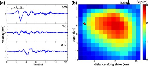
(a) The three component waveform data recorded at BAM station. The NF window covers the near-field P portion, and the S window covers the S-wave portion of the E–W seismogram. (b) Slip model taken from Funning et al. (2005) obtained from InSAR data. Red star is the hypocentre and black triangle shows the location of the BAM station.
This strong motion record was studied by Bouchon et al. (2006), who, through forward modelling, inferred a rupture velocity close to the Rayleigh wave velocity of the upper crust where rupture was confined.
There are three sets of parameters that characterize the seismic radiation from the earthquake; the slip distribution, the rupture arrival time at each point which is typically characterized by the rupture velocity and the time history of slip at each point which is commonly characterized by a slip-rate function. Slip distribution was independently determined from InSAR data by Funning et al. (2005), as shown in Fig. 1(b). The rupture velocity and slip-rate function are both assumed to be constant along the fault.
We first demonstrate the sensitivity of the near-field P and S waveforms to slip-rate function for the Bam earthquake by generating waveforms using various triangular-shaped source–time functions with rupture velocity fixed to 92 per cent of the shear wave speed (Fig. 2). As seen in Fig. 2, the rise and fall durations of the slip-rate function are critical in determining the transverse component waveforms. The sharper slip-rate functions accumulate moment more rapidly, yielding a higher amplitude near-field P phase. The pulse width and the peak of the later S-wave pulse also depend on the rise and fall durations of the slip-rate functions. This forward test clearly shows that the transverse ground motion contains crucial information about the slip-rate function.
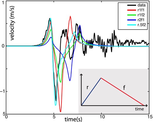
Data and model prediction of transverse component of velocity at BAM station, using four different triangular slip-rate functions and a rupture velocity of 92 per cent of shear wave velocity. Inset shows the triangular shape of the slip-rate function used for the forward models, where ‘r’ represents the rise (acceleration duration) and f represents the fall (deceleration duration) of slip velocity, for example, r1f2 is a triangular function with rise duration of 1 s and fall duration of 2 s.
2.3 The inversion method
In order to determine the shape of the slip-rate function and the rupture velocity, we go a step further in the analysis. We employ a Bayesian approach, where the goal is to find the family of slip-rate functions and the range of rupture velocity that produce waveforms which fit the observed near-field P waves and the S waves on the transverse component of the BAM recording. We use the slip distribution obtained from InSAR data by Funning et al. (2005), hence the only unknowns in the problem are the rupture velocity and slip-rate function, which are kept constant for all the sub-faults.
First, we generate a random set of slip-functions in certain time ranges, and a random set of rupture velocities. For each forward calculation we randomly select a slip-function and a rupture velocity in the pre-set ranges of parameters. Once the rupture velocity and the slip-rate function are chosen, with the predetermined slip distribution we calculate a forward model. We have generated 20 000 such forward models. Then the set of models are resampled by their fit to the near-field P and S pulse on the transverse component recording of the BAM station. We ignore the other two components, since not only they do not record any significant motion but also are sensitive to the details such as dip slip component of the rupture and other secondary source details and structural complexities.
2.4 Step 1: Generation of the slip-rate functions and the rupture velocities
For each forward model, a rupture velocity is randomly chosen between 74 and 94 per cent of the shear wave velocity. The prior distribution of randomly generated rupture velocities are shown in Fig. 4(a).
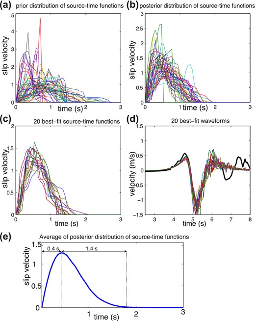
The results of the Bayesian sampling for σ2 = φmin. (a) 50 randomly selected slip-rate functions from the prior distribution of slip-rate functions. (b) 50 randomly selected slip-rate functions from the posterior distribution of models. (c) 20 best-fitting slip-rate functions. (d) 20 best-fitting waveforms where black is the data and the fits are shown in colours. (e) The average of the all posterior distribution of slip-rate functions.
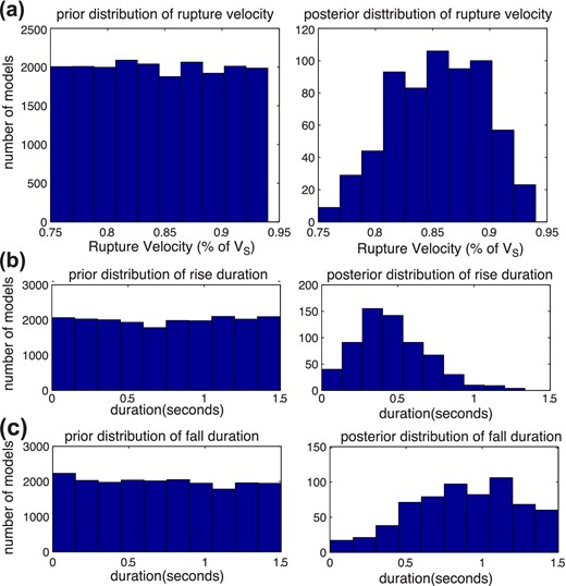
(a) Prior (left-hand side) and posterior (right) distribution of rupture velocity (b) Prior (left-hand side) and posterior (right-hand side) distribution of rise (acceleration) duration (c) prior (left-hand side) and posterior (right-hand side) distribution of fall (deceleration) duration.
Slip-rate functions are generated by randomly choosing rise and fall durations in a given time range (0–1.5 s). The only restriction on the slip-rate function is that it is forced to increase monotonically until a peak slip velocity, and decrease monotonically until the slip stops. This implies a single rupture front.
The construction of the slip-rate function is done in the following manner: Two random numbers are selected between 0 and 1.5 s which represent the peak velocity time (the acceleration or rise duration) and end time minus peak velocity time (deceleration or fall duration). In order to randomize the shapes of the functions, 10 random points are generated and sorted, which represent the random time steps that the slip-rate function increases to the peak velocity. Similarly the decrease from peak velocity to zero velocity is obtained at 10 random steps. 50 randomly generated slip-rate functions are shown in Fig. 3(a), and the prior distribution of rise and fall durations is shown in Figs 4(b) and (c).
2.5 Step 2: Calculation of the waveforms
Using the slip distribution obtained from geodesy, randomly generated slip-rate function and the rupture velocity as described in Step 1, we generate synthetic seismograms using the 1-D velocity structure inferred for the region by Tatar et al. (2005) and as previously used by Bouchon et al. (2006) (Table 1). The Green's functions are computed using the discrete wavenumber method (Bouchon 1981).
The 1-D upper crustal velocity structure from Tatar et al. (2005) which is used in this study.
| Thickness (km) | Vp (km s–1) | Vs (km s–1) | ρ (g cm–3) | Qp | Qs |
|---|---|---|---|---|---|
| 8.0 | 5.3 | 3.06 | 2.5 | 300 | 150 |
| 4.0 | 6.17 | 3.56 | 2.8 | 500 | 250 |
| 8.0 | 6.5 | 3.8 | 2.9 | 800 | 400 |
| Thickness (km) | Vp (km s–1) | Vs (km s–1) | ρ (g cm–3) | Qp | Qs |
|---|---|---|---|---|---|
| 8.0 | 5.3 | 3.06 | 2.5 | 300 | 150 |
| 4.0 | 6.17 | 3.56 | 2.8 | 500 | 250 |
| 8.0 | 6.5 | 3.8 | 2.9 | 800 | 400 |
2.6 Objective function and resampling
3 RESULTS
We generated 20 000 forward models which span the parameter space of possible slip-rate functions and rupture velocities. By resampling as described before, we obtain a posteriori probability density function (PDF) of accepted models.
In Figs 3(a) and (b), we show 50 randomly selected slip-rate functions from the prior and the posterior distribution, respectively. Fig. 3(c) shows the best-fitting 20 slip-rate functions and Fig. 3(d) shows their fit to the transverse component of the data. The results shown in Fig. 3 indicate that the type of slip-rate function that fits the near-field P and the S wave data is characterized by a sharp acceleration and slower deceleration. The models with slower acceleration phase do not accumulate the moment fast enough to explain the near-field phase.
Another way to inspect the obtained slip-rate function is to calculate the average of all the accepted models. The obtained average slip-rate function has acceleration duration of 0.4 s and deceleration duration of 1.4 s (Fig. 3e).
The asymmetry of the slip-rate function and plausible range of rupture velocity can also be inferred by comparing the distribution of the prior and posterior distribution of rupture parameters (Fig. 4). Fig. 4(a) shows the prior and posterior distribution of rupture velocities. The plausible range of rupture velocities is inferred as 82–90 per cent of the shear wave velocity, which is slightly less than the Rayleigh wave velocity. The characteristics of the slip-rate functions can be deduced from the posterior distribution of the rise and fall durations. The rise durations have a clear peak around 0.3–0.5 s, while the fall durations are harder to constrain with a broad range of solutions between 0.5 and 1.5 s (Figs 4b and c).
These results clearly reveal that the acceleration phase is faster than the deceleration phase, so the slip-rate function is asymmetric. The fall duration is harder to constrain, since it entails the later part of the seismogram and the smaller energy release at the very end of slip at a point does not lead to much radiation.
4 DISCUSSION
4.1 Robustness of the results
One critical issue is to ensure the robustness of our result for the Bam Earthquake case example. When the Bayesian resampling is performed; we use the minimum misfit rather than the data covariance in the formulation for the maximum likelihood solution. In order to test the effect of this arbitrariness, we try σ2 = 2φmin and |$\sigma ^2 = \frac{1}{2}\varphi _{{\rm min}} $| as two end member choices, and perform the resampling and obtain the posterior PDF (see Figs S3 and S4).
For |$\sigma ^2 = \frac{1}{2}\varphi _{{\rm min}} $| (Fig. S3), PDF becomes sharper, which means that we select less of the models that do not fit the data. When |$\sigma ^2 = \frac{1}{2}\varphi _{{\rm min}} $|, the a posteriori distribution of rupture parameters shows that the rupture velocity is 87–91 per cent of the shear wave velocity, the peak of the rise duration is about 0.3 s and the peak for the fall duration is 1.2–1.3 s. Hence, if we impose a sharper peak around the best-fitting model, the rupture velocity is closer to the Rayleigh wave velocity. The average slip-rate function does not change significantly.
For σ2 = 2φmin (Fig. S4), PDF becomes broader; therefore, more of the models that do not fit the data are included in the posterior PDF. Even in this case there is some constraint on the rupture velocity and slip-rate function. The rupture velocity is 80–90 per cent of the shear wave velocity and the peak of the rise duration is around 0.3–0.4 s. For the fall duration, any duration longer than 0.5 s seems plausible. The average slip-rate functions obtained from posterior distribution are very similar to the ones obtained for σ2 = φmin and |$\sigma ^2 = \frac{1}{2}\varphi _{{\rm min}} $|.
The acceleration duration can be better constrained due to the sensitivity of the near-field P phase to how fast the moment is accumulated. The deceleration duration is harder to constrain, since it produces the later parts of the seismogram where there is more trade-off. In addition, the smooth low amplitude ending part of the slip-rate function releases very small energy and does not add much to the seismic radiation, making it harder to constrain.
4.2 Implications for the slip-rate function
The theoretical solution of Kostrov (1964) for a self-similar crack implies a square-root singularity, followed by a longer deceleration where the slip-rate function goes to zero only after the crack stops and sends back healing pulses. For pulse-like ruptures, a similar truncated function is obtained by Nielsen & Madariaga (2003).
On the other hand, as mentioned before, the slip-rate function is very hard to retrieve from observations of seismic data (Cohee & Beroza 1994; Guatteri & Spudich 2000). Recognizing this lack of resolution, some of the kinematic modelers preselect a slip-rate function and use one or two parameters to obtain the duration of the slip-rate function, which is also referred to as ‘the rise time’. Amongst these commonly used slip-rate functions are two parameter cosine function (e.g. Ji et al.2002; Liu et al.2006), single parameter smooth ramp (Cotton & Campillo 1995; Bouchon et al.2002) or triangular function (Cohee & Beroza 1994).
Although various slip-rate functions are successfully adopted to fit the near-source waveforms in the typical frequency range (∼2–0.02 Hz) in conventional finite-fault modelling, these assumed slip-rate functions imply different earthquake source properties. One difference is that different slip-rate functions generate significantly different high frequency content (>1 Hz) (Guatteri & Spudich 2000). The choice of slip-rate function also leads to differences in estimation of dynamic parameters such as Dc (Guatteri & Spudich 2000; Tinti et al.2005).
Another important concern is that the slip-rate functions that are commonly used for source studies have different spectral decays, which would imply different source scaling relationship. Mena et al. (2010) compared the spectral decays of various slip-rate functions adopted by finite-fault modellers and showed that the spectral decay of the slip-rate function can be 1/f, 1/f2 or even of higher order. They preferred the slip-rate function of Dreger et al. (2007) which has 1/f spectral decay. For Haskell type source model (1964; Brune 1970) where the far-field displacement spectral decay is 1/f2, the rise time has to decay as 1/f, since another 1/f factor will arise from the finite propagation of the rupture.
Fig. 5(a) shows the spectral decay of the slip-rate function for the 2006 Bam Earthquake, which is the average of the 100 best-fitting slip-rate functions. The spectrum of our best-fitting slip-rate function is consistent with a 1/f2 spectral decay. This implies that although the slip-rate function that we obtain is asymmetrical as expected by dynamic simulations, the slip rate is function is broad around the peak so that the spectral decay is 1/f2.
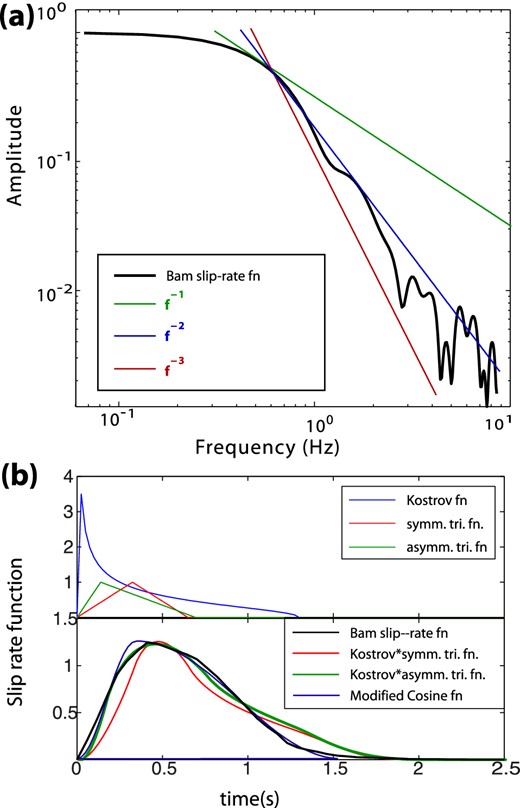
(a) The spectrum of the average of the 100 best-fitting slip-rate functions obtained for the 2003 Bam earthquake in comparison with 1/f, and 1/f3 spectral decays. (b) (top) A Yoffe function (blue) and the symmetric (0.325 s half-width) and asymmetric (green) triangular (0.2 s rise–0.5 s fall) functions that are used for convolution. (bottom) The slip-rate function for the Bam earthquake compared with the regularized Yoffe functions convolved with the symmetric and asymmetric triangles and also the two parameter cosine function.
Tinti et al. (2005) have suggested a two- parameter function, referred to as ‘Regularized Yoffe function’, which is motivated by dynamic models and is coherent with the scaling between kinematic and dynamic parameters obtained from numerical modelling assuming slip-weakening law and laboratory experiments (Ohnaka et al.1987). The proposed regularized Yoffe function, is a truncated Kostrov function which is convolved with a triangle to avoid singularity at the crack tip.
Here we compare the Bam earthquake slip-rate function with the regularized Yoffe function proposed by Tinti et al. (2005) and also with the 2 parameter modified cosine function which is also commonly used (Ji et al.2003; Liu et al.2006). Fig. 5(b) shows the Kostrov function truncated at 1.3 s and symmetric and asymmetric triangular functions which we have convolved to obtain the regularized Yoffe functions. Fig. 5(c) shows the comparison of the Bam slip-rate function with the regularized Yoffe functions and the two parameter cosine function. We found that when a symmetrical triangular function (width of 0.65 s) is convolved with the Kostrov function, the similarity between the regularized Yoffe function and the Bam earthquake slip-rate function is limited. When a narrower triangular function is used, observed broadness of the slip-rate function is hard to obtain. When a larger triangle is used for convolution, the rapid acceleration that is observed becomes hard to retrieve. Therefore, we add one more parameter and convolve the truncated Kostrov function with an asymmetric triangle (0.15 s rise and 0.55 s fall duration) and find a similar functional shape with the observed average slip-rate function. Fig. 5(c) shows that it is also possible to approximate the Bam slip-rate function with a two-parameter cosine function with 0.3 s rise and 1.1 s fall duration.
This test shows that although the asymmetry of the slip-rate function is clear, which favours solutions that are consistent with dynamic simulations, one cannot choose between different asymmetric parametrizations at this point. It would require studies of more earthquakes with near-source data to come up with family of solutions of slip-rate functions that fit the observations.
It is important to note that in this study we obtain an average slip-rate function for the whole fault rupture. Since there is only one record, it is not possible to obtain a detailed map of slip-rate function variation along the rupture. In future cases, where there might be multiple strong-motion records of earthquakes, using the techniques described here, it will be possible to obtain the variations of the slip-rate functions along the fault. When more observations accumulate, we will have a much better understanding of how to parametrize the slip-rate function. In addition, the variation of slip-rate function along the fault will significantly contribute to our understanding of physics of the rupture.
4.3 Implications for earthquake dynamics
One of the simple models of friction is the slip-weakening law, which assumes a linear decrease from yield strength to sliding friction, depending only on the accumulated slip (Ida 1972; Andrews 1976a,b). The characteristic slip, at which the friction coefficient decreases to the sliding friction, is called the slip-weakening distance (Dc). Mikumo et al. (2003) have shown that the time of the peak slip velocity is related to the slip weakening distance especially away from the edges of the slip areas (Fukuyama et al.2003). Therefore, the slip-rate function can be used to infer the slip weakening distance. Assuming an average slip of 2.5 m inside the main asperity implies a Dc ∼ 85 cm. This is in the same order of magnitude as the one obtained by Mikumo et al. (2003), for the 2000 Mw6.7 Tottori Earthquake (Dc ∼70–90 cm) and 1995 Mw7.2 Kobe Earthquake (Dc ∼40–90 cm). Peyrat et al. (2001), used 80 cm for the dynamic simulation of the 1992 Mw7.3 Landers Earthquake.
The total duration of the average rise time is shorter than 2 s, and most of the slip occurs during the first 0.5 s. Considering an average rupture velocity of 2.75 km s–1, and fault length of 15 km, the rupture duration is about 5.5 s. This is longer than the slip-rate function obtained here implying a pulse-like rupture propagation as Heaton (1990) has shown for many earthquakes.
4.4 Implications for the objective function
One critical element of kinematic modelling of earthquakes is choosing the objective (cost) function which determines the error that is to be minimized. Common practice is to use the L2 norm which is also consistent with Gaussian errors and Euclidean definition of distance (Hartzell & Heaton 1983). Alternatively the inversion can be done in frequency domain (Cotton & Campillo 1995) or wavelet domain (Ji et al.2002), in order to express the importance of various frequency bands and phase arrivals.
Although the amplitude of the near-field phases is smaller than the following S waves, they are of great importance due to their sensitivity to the moment accumulation. When standard L2 norm objective function is used, the contribution of the misfit to the near-field phase to the overall misfit is not significant in comparison to the following much larger amplitude S-wave pulse or later phases which might occur due to source or structural complexities. In fact, if we had used a standard L2 norm and all three components of the seismogram, the later pulse observed due to a secondary thrust faulting on the vertical component would have contributed more than the near-field phase on the E–W component (Fig. 1). The resolution in our analysis comes from adding weight to the near-field phases, as well as ignoring the later phases which might be present due to details of the structure or source. We suggest that an objective function that considers the sensitivity of various phases and emphasizes the beginning of the seismograms can be more suitable for inferring kinematic parameters.
4.5 Implications for strong-motion station locations
The near-field phases can only be observed at stations that are close to the fault rupture, since the amplitude of the near-field phases decays more rapidly (with 1/r2) in comparison to the far-field phases (1/r). Considering their importance in determining the source properties, it would be useful to get a sense of how close one should install the strong-motion seismometers to the fault lines in order to observe clean near-field phases.
In general, how far the near-field phases can be reliably recorded depends on the moment accumulation and fault geometry. Here, we would like to use the Bam example to quantify how close one should install strong-motion stations to capture these near-field phases for an event like the 2003 Bam Earthquake. The value we obtain might be valid for earthquakes similar to the Mw6.6 Bam Earthquake and larger ones.
We calculated the synthetic transverse seismograms along a profile that passes through the Bam station (Fig. S5). We used the slip distribution of the Bam earthquake as before, and an asymmetrical triangular slip-rate function with rise of 0.5 s and fall of 2 s. We calculated the transverse component seismograms at 0.4, 0.8, 1.2, 1.6, 2, 2.5 and 3 km (Fig. S5b). The transverse seismograms show that the near-field phase has significant amplitude only up to 2 km distance from the fault line. After 2 km, the near-field phase is of significant amplitude, while the following S wave pulse amplitude does not decrease significantly since it is a far-field phase. Hence one can infer that for an earthquake of Mw6.6 or larger, stations as far as 2 km can be used in for studying the near-field phases.
5 CONCLUSION
We obtained an average slip-rate function from kinematic inversion by using near-field P phase and S phase of the transverse component record of the 2003 Mw6.6 Bam Earthquake. Our method emphasizes the sensitivity of the near-field phase to moment accumulation, which depends both on slip-rate function and rupture velocity. We propose that a modified objective function that emphasizes near-field phases and the following transverse S waves will help constrain source parameters more effectively. The average slip-rate function obtained for the 2003 Bam Earthquake has acceleration duration of 0.4 s and deceleration duration of 1.4 s. This rapid accumulation of slip is consistent with dynamic models which predict a rapid acceleration and slower deceleration. The short duration of the slip-rate function relative to the rupture duration implies that the Bam Earthquake propagated as a pulse-like rupture. In future cases where multiple near-source records exist for an earthquake and slip distribution can be constrained independently from geodesy, this method can be used to obtain a detailed map of slip-rate functions and its variations along the fault, which would contribute significantly to our understanding of rupture dynamics.
This manuscript has benefited significantly from detailed comments from two reviewers, Prof Douglas Dreger, Prof Minoru Takeo and the editor Prof Eiichi Fukuyama. We would like to thank Prof Hayrullah Karabulut and Dr Yeliz Utku Konca for their help in improving the manuscript.
REFERENCES
SUPPORTING INFORMATION
Additional Supporting Information may be found in the online version of this article:
Figure S1. (a) The slip distribution of the synthetically generated Mw6.9 earthquake used for this test. (b) The location of stations (green triangles) with respect to the fault (red line), the hypocentre is shown with a red star. (c) The transverse component velocity seismograms at stations along the fault using rupture velocities of 2, 2.5 and 3 km s–1 and various triangular slip-rate functions. ‘r’ and ‘f’ represent the rise and fall durations of the triangular functions, similar to Fig. 2.
Figure S2. (a) The transverse component velocity seismograms along the fault for 1 m (red), 2 m (black) and 3 m (blue) of slip. (b) The station distribution and the location of the fault (blue line). The red star shows the hypocentre location. (c) The slip distribution used for the calculation. The red sub-faults demonstrate the slipping area with 1, 2 and 3 m slip, respectively. The rupture velocity is 2.5 km s–1 and rupture time contours are shown every 2 s. The slip-rate function is a symmetric triangular function with a width of 2 s.
Figure S3. The results of the Bayesian sampling for |$\sigma ^2 = \frac{1}{2}\varphi _{{\rm min}} $|. (a) 50 randomly selected slip-rate functions from the prior distribution of models. (b) 50 randomly slip-rate functions from the posterior distribution of models. (c) 20 best-fitting slip-rate functions. (d) 20 best-fitting waveforms where black is the data and the fits are shown in colours. (e) Prior (left-hand side) and posterior (right-hand side) distribution of rupture velocity. (f) Prior (left-hand side) and posterior (right-hand side) distribution of rise (acceleration) duration. (g) Prior (left-hand side) and posterior (right-hand side) distribution of fall (deceleration) duration. (h) The average of the all posterior distribution of slip-rate functions.
Figure S4. The results of the Bayesian sampling for σ2 = 2φmin. (a) 50 randomly selected slip-rate functions from the prior distribution of models. (b) 50 randomly slip-rate functions from the posterior distribution of models. (c) 20 best-fitting slip-rate functions. (d) 20 best-fitting waveforms where black is the data and the fits are shown in colours. (e) The average of the all posterior distribution of slip-rate functions. (e) Prior (left-hand side) and posterior (right-hand side) distribution of rupture velocity. (f) Prior (left-hand side) and posterior (right-hand side) distribution of rise (acceleration) duration. (g) Prior (left-hand side) and posterior (right-hand side) distribution of fall (deceleration) duration.
Figure S5. (a) Slip distribution and the station distribution, at which the transverse seismograms are calculated. The profile is along the actual location of the BAM station shown by the nearest station (blue triangle). (b) The calculated transverse seismograms at stations along the profile (Supplementary Data).
Please note: Oxford University Press is not responsible for the content or functionality of any supporting materials supplied by the authors. Any queries (other than missing material) should be directed to the corresponding author for the article.
