Assimilation of Deformation Data for Eruption Forecasting: Potentiality Assessment Based on Synthetic Cases
 M. Grace Bato
 Virginie Pinel
 Yajing Yan
- 1ISTerre, IRD, Centre National de la Recherche Scientifique, Université Savoie Mont-Blanc, Le Bourget du Lac, France
- 2LISTIC, Université Savoie Mont-Blanc, Annecy-le-Vieux, France
In monitoring active volcanoes, the magma overpressure is one of the key parameters used in forecasting volcanic eruptions. This parameter can be inferred from the ground displacements measured on the Earth's surface by applying inversion techniques. However, in most studies, the huge amount of information about the behavior of the volcano contained in the temporal evolution of the deformation signal is not fully exploited by inversion. Our work focuses on developing a strategy in order to better forecast the magma overpressure using data assimilation. We take advantage of the increasing amount of geodetic data [i.e., Interferometric Synthetic Aperture Radar (InSAR) and Global Navigation Satellite System (GNSS)] recorded on volcanoes nowadays together with the wide-range availability of dynamical models that can provide better understanding about the volcano plumbing system. Here, we particularly built our strategy on the basis of the Ensemble Kalman Filter (EnKF). We forecast the temporal behaviors of the magma overpressures and surface deformations by adopting a simple and generic two-magma chamber model and by using synthetic GNSS and/or InSAR data. We prove the ability of EnKF to both estimate the magma pressure evolution and constrain the characteristics of the deep volcanic system (i.e., reservoir size as well as basal magma inflow). High temporal frequency of observation is required to ensure the success of EnKF and the quality of assimilation is also improved by increasing the spatial density of observations in the near-field. We thus show that better results are obtained by combining a few GNSS temporal series of high temporal resolution with InSAR images characterized by a good spatial coverage. We also show that EnKF provides similar results to sophisticated Bayesian-based inversion while using the same dynamical model with the advantage of EnKF to potentially account for the temporal evolution of the uncertain model parameters. Our results show that EnKF works well with the synthetic cases and there is a great potential in using the method for real-time monitoring of volcanic unrest.
1. Introduction
Tracking the migration of magma as it propagates to the Earth's surface is crucial in eruption forecasting as well as in volcanic hazard assessment. When magma accumulates at shallow depth or propagates toward the surface, it induces seismicity as well as surface displacements, such that geophysical signals recorded at volcanoes have long been used to infer magma path and magma plumbing system characteristics (e.g., Swanson et al., 1983; Voight et al., 1998; Aoki et al., 1999; Roult et al., 2012; Sigmundsson et al., 2015). Recently the ability of geodesy to provide continuous and spatially extensive evolution of surface displacements during inter-eruptive periods has been drastically improved as a consequence of the increasing number of continuous Global Navigation Satellite System (GNSS) networks installed on volcanoes (e.g., Geirsson et al., 2012; Peltier et al., 2016) together with the improvement of the availability of Synthetic Aperture Radar (SAR) data (i.e., better spatial coverage, improved spatial and temporal resolution of SAR data from new satellite missions) (e.g., Pinel et al., 2014). This progress allows to characterize the geometry of magmatic plumbing systems underlying volcanoes in terms of reservoir shapes, depths and numbers. In particular, at some specific volcanoes, deep magmatic reservoirs, which had been ignored so far, are evidenced (e.g., Elsworth et al., 2008; Chadwick et al., 2011; Bagnardi and Amelung, 2012; Hautmann et al., 2014; Tiampo et al., in press). However, most of the models used to interpret geodetic data are kinematic and cannot provide information on the pressure within the magmatic system, which is the key parameter to control the timing of magma reservoir rupture as well as the ability of magma to reach the surface and thus to feed an eruption. Besides, the difficulty to determine independently the size of a magma chamber and its pressure change has been recognized for many years (McTigue, 1987; Segall, 2013). Basically, the same displacement field is expected from a small pressure change affecting a large magma reservoir and from a large pressure change experienced in a small magma chamber. However, consequences are not the same as the latter case is more prone to end in a short-term eruption. The good point is that the temporal evolution of the displacement field should help deciphering between those two cases, considering similar magma and crustal rheologies, the pressurization of a small chamber being much quicker than for a large one. One limitation of this approach, as recently demonstrated by Segall (2016), is that the temporal evolution actually results from a convolution between the history of a pressure source and the magma and crustal rheology (Reverso et al., 2014). It follows that additonal observations such as gravity data might be useful to discriminate both effects.
In addition to the recent progress in geodetic observations, several dynamical models of magmatic system evolution have been recently derived. They provide an interpretation of the temporal evolution of geodetic data as well as seismic observations considering either the rheology of the encasing medium (Nooner and Chadwick, 2009; Carrier et al., 2014; Got et al., 2017) or the evolution of the magma inflow at the bottom (Lengliné et al., 2008; Pinel et al., 2010; Reverso et al., 2014). The latter type of models has proven to be useful in recovering information of the deepest part of the magma plumbing system, such as the size of the deep storage zone as well as the bottom magma inflow (Reverso et al., 2014), which is always quite difficult to constrain. Segall (2013) has nicely demonstrated the interest to combine deformation data and a physics-based model of the plumbing system with a Bayesian-based approach in order to forecast eruptions. In particular, the Markov Chain Monte Carlo method was applied with success to Mount St Helens (Anderson and Segall, 2011, 2013). As noticed by Segall (2013), a limitation of this approach is that it cannot account for epistemic uncertainties. Another limitation is potentially that it is not efficient to estimate model parameters evolving through time. Also, the challenge remains in accommodating incoming data and using them efficiently. Inversion methods are data intensive (i.e., uses all observations from the beginning) and typically requires expensive calculations at each observation period, hence may not be suitable for real-time eruption forecasting. To address these issues, data assimilation–a common method used in ocean-weather forecasting and monitoring–is here applied as a way to combine volcano deformation data and physics-based models.
Data assimilation is a time-stepping process that combines models, observations and a priori information based on error statistics to forecast the state of a dynamical system. It was initially developed in ocean-atmosphere science (e.g., Talagrand and Courtier, 1987; Talagrand, 1997; Houtekamer and Mitchell, 2005; Yan et al., 2014), and has gained popularity in many other fields of geosciences such as vegetation and soil moisture (e.g., Reichle et al., 2007; Barbu et al., 2011), natural resource exploration (e.g., Lorentzen et al., 2001; Geir et al., 2003; Gu and Oliver, 2005; Chen and Oliver, 2010; Zoccarato et al., 2016) and geomagnetism (e.g., Fournier et al., 2007, 2010; Kuang et al., 2010; Gillet et al., 2015). Many assimilation algorithms are already available nowadays. Among them, is the Kalman Filter (KF). It was first introduced by Kalman (1960) and was regarded as the greatest achievement in estimation theory and control systems applications of the twentieth century, enabling the precise and efficient navigation of spacecrafts in the solar system (Grewal and Andrews, 2008). In earthquake research, KF has been used to determine fault slip evolutions (Segall and Matthews, 1997; McGuire and Segall, 2003; Bartlow et al., 2014; Bekaert et al., 2016). At active volcanoes where nonlinear processes are typical, variants of KF have been used in order to solve nonlinear equations. For example, Fournier et al. (2009) used unscented KF to track the magma recovery at Okmok, but the strategy is strongly dependent on assumptions such as initialization task and selection of hyperparameters that are typically problem-dependent (Julier and Uhlmann, 2004; Shirzaei and Walter, 2010). Shirzaei and Walter (2010) coupled genetic algorithm with KF to monitor volcano source at Campi Flegrei, which requires rerunning of KF for several times. In all these studies in the Earth Science field, the KF is used as a temporal filter without considering any forward dynamical model. So far, the application to volcanology of the KF based on a dynamical model has been restricted to one study (i.e., Gregg and Pettijohn, 2016) using a forward model accounting for a viscous rheology of the encasing medium. However, the model parameter controlling the temporal evolution of the medium and the crustal viscosity was in this study considered as a fixed parameter, thus limiting the interest of considering the temporal evolution of the system. Also, their approach was based on a finite element model which limits the application to real-time forecasting and their joint assimilation of GNSS and InSAR data was still problematic.
In this work, our main goal is to test the ability of Ensemble Kalman Filter (EnKF) to quantify the magma pressure evolution at depth from surface displacement data and thus to forecast pressure-based volcanic eruptions. As a first attempt, we focus on a specific dynamical model that well-describes the behavior of several often erupting basaltic volcanoes. We developed an efficient approach to assimilate GNSS and InSAR data into a two-magma reservoir model, which is a simple and generic dynamical model for the magma plumbing system, in order to forecast the overpressures and to constrain two model parameters related to the deepest part of the reservoir system. We begin by briefly discussing the two-magma reservoir model of Reverso et al. (2014) in Section 2, then reviewing the fundamentals of the EnKF approach in Section 3, followed by the experiment setup and the step-by-step implementation of our EnKF strategy in Section 4. We then present two synthetic cases (i.e., case A and case B) when considering the magma inflow at the bottom of the system as well as the size of the deepest reservoir as uncertain and given two kinds of initial conditions about the uncertain parameters (i.e., biased or unbiased distribution). In particular, case A is about state estimation wherein we only track the behavior of the overpressures, while case B demonstrates state-parameter estimation where the uncertain model parameters are estimated in parallel with the overpressures. In the discussion part, we tackle the effects of the spatial and temporal characteristic of the datasets (i.e., GNSS-like and InSAR-like data) used during the assimilation and how far-field data affect the performance of assimilation. We also compare the performance of EnKF with a Bayesian-based inversion. Then we present the advantages and limitations of the dynamical model we considered as well as the possibility of applying data assimilation to other types of models. Lastly, we discuss the ease of implementing our strategy and the future of EnKF for real-time volcano monitoring.
2. Forward Dynamical Model
We use the two-magma reservoir model proposed by Reverso et al. (2014). This model consists of two reservoirs embedded in an elastic medium and connected by a hydraulic pipe. The deeper reservoir is assumed to be fed by a constant magma inflow, which corresponds to the bottom boundary condition of the system. The magma is assumed to be incompressible. This model, presented on Figure 1, is characterized by a set of geometrical and rheological parameters listed in Table 1 and solves for the temporal evolution of the magma overpressures, ΔPs and ΔPd, for the shallow and the deep reservoirs, respectively. As shown by Reverso et al. (2014), this simple model provides a consistent explanation for the temporal evolution of the post-eruptive displacement measured at Grímsvötn volcano, Iceland after the three last eruptions (1998, 2004, and 2011). The initial and transient exponential behavior is due to the refilling of the shallow reservoir by the deeper one after the eruption. Then, once the system has been readjusted, a constant displacement rate is observed due to the constant magma inflow at the bottom of the system.
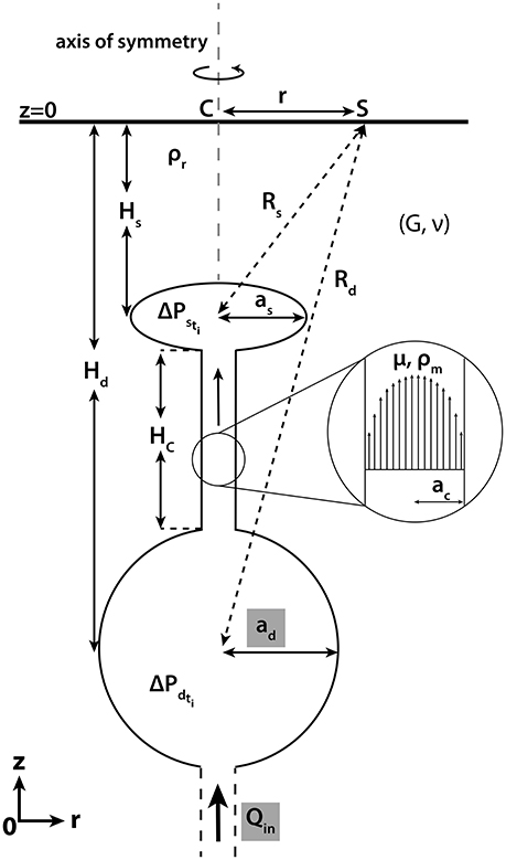
Figure 1. Schematic sketch of the two chamber model, modified after Reverso et al. (2014). The magma inflow rate at the bottom chamber Qin and the radius of the deep reservoir ad are the two parameters considered to be uncertain in this study. Observations (vertical and horizontal displacements) are recorded at the surface at a given location S characterized by its distance r from the center of the volcanic system C. and are distances between S and the shallow and deep reservoirs, respectively.
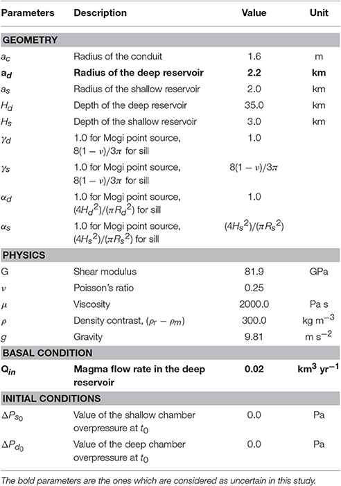
Table 1. Model parameters and true values assigned for the synthetic case.
In this model, the values of the overpressure within the shallow and deep reservoirs, respectively, ΔPs and ΔPd, at a given time ti+1 are derived from their values at the previous time step ti using the following discrete time-step equations (see equations derived in Appendix A of Reverso et al., 2014):
The shapes (i.e., spherical or sill-like) of the shallow and deep reservoirs are characterized by two geometrical constants, respectively, γs and γd (Reverso et al., 2014). The discrete formula stays valid as long as the time interval Δt = ti+1−ti remains small compared to the time constant τ of the system given by (Reverso et al., 2014). Note that when the bottom magma inflow rate Qin is set to zero and the deep reservoir is sufficiently large when compared to the shallower one (ad/as ≈ ∞), this model corresponds to the case of a unique magma reservoir fed by a deep magma source which remains at constant pressure as previously proposed for several basaltic volcanoes (Lengliné et al., 2008). This model can also represent the upper part of more complex plumbing system made of a large number of magma reservoirs lying at increasing depth. It thus benefits from the advantage of being both generic and simplistic.
Based on the Mogi model (Mogi, 1958), the radial uR and vertical uz displacements observed at the surface can be expressed using:
The shapes (i.e., spherical or sill-like) of the shallow and deep reservoirs are characterized by two geometrical constants, respectively αs and αd (Reverso et al., 2014). Provided that one has access to the deformation fields related to the activity of the volcano (i.e., inferred from GNSS observations and/or InSAR), Equations (3) and (4) create a link between the dynamical model and the observations, necessary for data assimilation.
3. Data Assimilation: Ensemble Kalman Filter
On one hand, forecasts given by a dynamical model incorporate errors due to the choices or limitations related to the model physics and parameters: including errors associated with assumptions, theory and/or conceptualizations within the underlying equations, errors due to the computational grid and its discretization, numerical errors related to the time-step or numerical methods used to solve the mathematical equations, and errors associated with the model parameters. On the other hand, uncertainties are also present in the observations due to the instrument itself, different perturbations during data acquisition, and noise generated during pre- and post-processing of data. Moreover, in most cases, observation is not spatially nor temporally complete because of the limitation in data acquisition. Data assimilation takes advantage of the complementary information provided by the dynamical model and the observations. It corrects model forecasts whenever observations are available in order to provide model state trajectory as accurate as possible. In ocean-atmosphere science, it has become the common approach for monitoring and forecasting.
Ensemble Kalman Filter is an ensemble-based stochastic data assimilation technique developed by Evensen (1994) and Evensen (2003) as an alternative route to solve the limitations of the classic Kalman Filter. The main characteristic lies on the use of N-ensemble of realizations to construct a Monte Carlo approximation of the mean and covariance of the state vector (i.e., vector containing all the model parameters to be improved by data assimilation).
We adopted the EnKF method in this paper. In general, the assimilation is divided into two steps: (1) the forecast step and (2) the update step (also known as the analysis step). The EnKF begins with the ensemble generation. N realizations (ensembles) of uncertain model parameters are performed according to an a priori distribution. Then, Monte Carlo simulation is performed while running forward the dynamical model for each ensemble member, resulting to the ensemble of model state forecast X, i.e., where Nx is the number of state variables and Nn is the ensemble size, and the associated covariance error Pf.
In the following section we further describe the EnKF scheme and equations based on Evensen (1994, 2003).
3.1. Forecast Step
The forecast is carried out by the model integration under the control of the model operator that represents the physical process governing the system. The model state at the current instance is forecasted from the model state at previous instance according to the model operator as expressed in Equation (5).
f and a: denote the forecast and analysis, respectively, : the model operator derived from Equations (1) and (2) that relates the state of the system at time, ti to ti+1 (see Appendices A,B), and q: the model error. Initial conditions of the model state variables are necessary to start the model.
At each time step, the error covariance Pf of the model forecast which is an Nx × Nx matrix can be obtained using:
3.2. Update Step
The update stage consists of correction of the model forecasts by the observations in order to obtain a more precise estimation of the model state. The observations D, i.e., where Nm is the total number of observations, can be anything that are related to the true model state x† by the observation operator .
Note that the observation error ϵ allows the derivation of the error covariance of the observations R, i.e., R = 𝔼(ϵϵT).
Updating Xf is straightforward and can be performed by first computing the Kalman gain K using Equation (8). The Kalman gain simply represents the magnitude of which the incoming observation corrects the model estimates in Equation (5).
To formalize the update, we use Equation (9).
The result of the update is called the analysis Xa. It is the linear sum of the model forecast and the correction introduced by the observation given the difference between the observations and model forecasts. In general, the analysis must be at least statistically as accurate as any of the individual observation or the model forecast.
Lastly, the error covariance of the analysis Pa is calculated using Equation (10).
4. Experiment Set-up
We will now describe in detail how the assimilation experiments are implemented. The state variables are the magma overpressures ΔPs and ΔPd within the shallow and deep magma reservoirs, respectively. The observations are the vertical and the radial surface displacements observed at a given time ti and at a given distance r from the axis of symmetry of the system. From a model simulation with a given set of parameters listed in Table 1 (see Section 4.1), we generate a set of synthetic observations and then using these observations and considering two of the parameters as uncertain, we perform the assimilation as described in Section 4.2 and compare the derived overpressures and model parameters obtained in two synthetic cases (i.e., state-only, state-parameter).
4.1. Generating Synthetic Observation
We perform a model simulation to produce synthetic data by setting each model parameter to a given value as defined in Table 1. In data assimilation, this step is referred to as the true run. These values are chosen such that they are consistent with the case of Grímsvötn volcano in Iceland. In particular, at Grímsvötn Volcano, the shallow storage zone has been well characterized by seismic and geodetic studies (Alfaro et al., 2007; Hreinsdóttir et al., 2014). Other geometrical parameters are chosen in consistent with the study of Reverso et al. (2014). The value taken for the shear modulus G however, represents an upper bound for the lower part of the crust (Auriac et al., 2014). This large value results in large magma overpressure values but it does not influence the interpretation of the assimilation technique.
To produce the synthetic overpressures, the analytical solution of Reverso et al. (2014) to the differential Equations (1) and (2) are used, i.e., :
with . The resulting overpressures are considered as the true values and are then used as input in Equations (3) and (4) in order to generate synthetic displacements , i.e., .
The observation is then generated by adding a white Gaussian noise, i.e., , to the synthetic displacements, where σu represents the instrument precision along the radial and vertical directions. We use the typical GNSS instrument errors that are 1 and 10 mm for uR and uz, respectively.
Figure 4 shows the observations (vertical and radial displacements) generated at various distances from the volcanic center (i.e., r = 1 to 4.9 km). Notice that for all the radial displacements and for those vertical displacements that are nearest to the volcano axis (i.e., r = 1 to 2.5 km), it is very difficult to discern the synthetic observation because the amplitude of the noise is very small relative to the signal. Note that in the results part (Section 5) we use a total of 80 observations (i.e., Nm = 80) to define the observation vector D, which comprises the vertical and radial displacements, uniformly (every 100 m) located at distance r = 1 to 4.9 km away from the volcano axis. The effect of the number of observations used as well as the frequency of incoming observations are discussed in Section 6.1.1.
4.2. Assimilation Strategy: Using EnKF
The state variables are the overpressures ΔPs and ΔPd and we consider two parameters, the radius of the deep reservoir ad and the basal magma inflow rate Qin as uncertain. We focused on these particular parameters characterizing the deeper part of the magma plumbing system because they are the most difficult to recover using surface displacement data.
The time interval Δt is fixed to 2 days, which is much smaller than the true time constant τ (i.e., τ = 0.11 yr). The start of the assimilation begins just after an eruption when the reservoirs are refilling and terminates after 500 time-steps (i.e., tf ~ 2.74 yr). The initial values of magma overpressures are set to zero (See Table 1), assuming that both reservoirs had been fully depressurized by the previous eruption (i.e., the magma pressures within the reservoirs equal the surrounding lithostatic one). The frequency of available observation fobs is usually fixed to one; meaning that at each assimilation step (i.e., every 2 days) there is always an available observation. In the case where no observation (fobs = 0) is available, the model forecast cannot be corrected by the observation. This particular case is hereafter called the free run and is presented for comparison.
Two cases are considered here: case (A) where we only forecast the state variables and case (B) where the state variables and the two uncertain parameters (ad and Qin) are both estimated. We used the classic EnKF where the observations are perturbed prior to assimilation (Burgers et al., 1998). Below we describe in detail the practical implementation of EnKF as summarized in Figure 2:
1. We start by defining an initial ensemble of 1,000 members. For ensemble generation, two distributions are considered for the uncertain parameters: (1) using a truncated-Gaussian distribution wherein the mean of each distribution is centered on the true value of the uncertain parameters (hereafter called unbiased) and (2) using a Gaussian-prior distribution that does not include the true value of the uncertain parameters, the mean of each distribution being very far from their true values (hereafter called biased).
2. For each of the ensemble members:
a. We run the forward model step-by-step from the initial condition until the data assimilation step ti+1. The state vector is built depending on which case is being tested. See Appendices A,B for the state-only estimation and state-parameter estimation, respectively.
Tip 1: When performing either state-only estimation or state-parameter estimation, an inflation factor ρinfl ∈ [0, 1] can be multiplied to the ensemble of state variables, i.e., , to prevent the ensemble from collapsing to a single value. For all the synthetic cases performed (Section 5), we used an inflation factor equal to 0.1 at each assimilation step.
Tip 2: In state-parameter estimation using EnKF, the parameters are only updated by the covariance between them and the state variables. When doing so, we randomly perturb the uncertain parameters by adding noise, , where αp is the additive inflation. This would help the filter to explore more possible values since their values do not change during the forecast step, i.e., . In our synthetic cases, we used an additive inflation of αad = 5 and αQin = 0.005 to tune the uncertain parameters during the assimilation. These are derived from empirical observations after several adjustments.
b. The error covariance of the forecast Pf is computed using Equation (6).
c. We perturb the field observation vector using:
where η is a random variable with distribution .
d. The state vector is then updated using Equation (9), replacing D with :
Tip 3: Resample the analysis state vector Xa using the strategy proposed by Evensen (2009) before moving to the next data assimilation time step if the updated values of the uncertain parameters fall beyond or exceed the boundary conditions.
e. The error covariance of the analysis Pa is obtained using Equation (10).
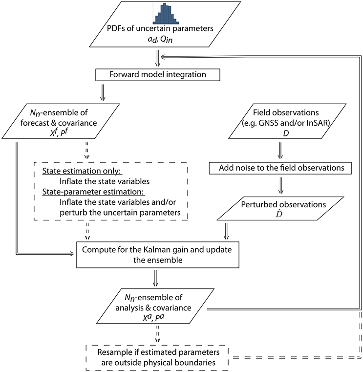
Figure 2. The step-by-step EnKF strategy that we implemented in this study. The broken borders and lines imply that the step is optional.
5. Results
5.1. Synthetic Case A: State Estimation
The first test case tracks only the evolution of the overpressures in the shallow and deep reservoirs, i.e., Equation (A1), given an initial condition where the distributions of the uncertain parameters are unbiased (Figure 3C) or biased (Figure 5C).
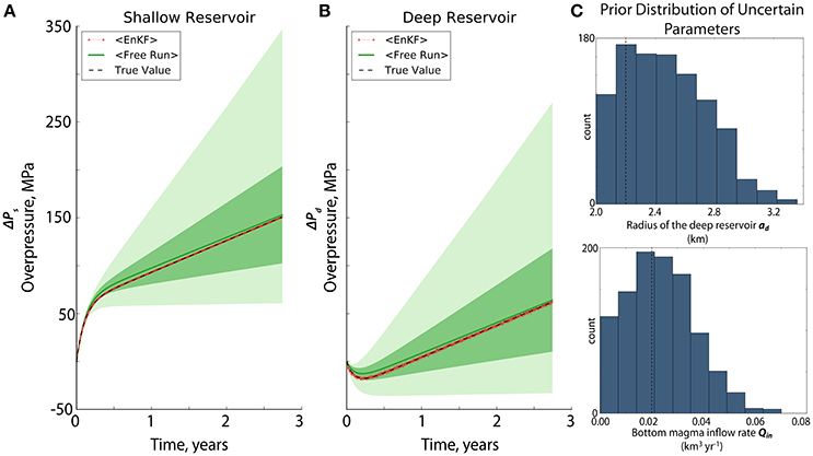
Figure 3. The evolution of the overpressures after performing the state estimation (A,B) given that the initial ensemble of the uncertain parameters (C) are non-Gaussian, centered on their true values (black broken lines). In (A,B) the black broken line represents the true value of the overpressures. The green ones represent the model forecasts where the green solid line is the mean, the dark green fill is the spread (1σ) and the light green fill covers the full extent of the ensemble (i.e., [min, max]). The red ones represent the result of EnKF where the red solid line is the mean, the dark red fill is the spread (1σ) and the light red is the full extent of the ensemble. Notice that the spread of the ensemble is very narrow for the assimilation case (~104–106).
In both cases, the EnKF performed well in forecasting the shallow and deep overpressures toward the end of the assimilation as evidenced by the red line (i.e., EnKF) that closely follows the black broken line (i.e., true value) in Figures 3, 5. In fact for the shallow overpressure, even with a poor knowledge about the uncertain parameters, the EnKF was able to catch almost perfectly the true overpressure. Unsurprisingly, the overpressure forecast for the deep reservoir is more likely affected by poor parameter initialization because the displacement induced by the deeper chamber is smaller, such that its overpressure is indirectly constrained by the dynamical model and consequently more influenced by the two uncertain parameters.
In Figure 5B, the result of EnKF is found closer to the free model forecast (i.e., results in green, labeled as free run) at the start of the experiment when the prior information about the uncertain parameters is far from their true values (see inset 2 for a magnified version). The model error seems smaller at the beginning as compared to the observation error, hence, the contribution of the model forecast is found to dominate the process. As the experiment goes on, the model error increases tremendously (i.e., the mean overpressure from the free run deviates away from the true overpressure) but thanks to the small measurement error, the analysis was able to converge closer to the true state of the system. Although overpressure estimation may have been unsuccessful toward the end of the assimilation, still, the resulting error differences between the true values and the EnKF-estimates are very small (i.e., 0.69% and 4.25% for the shallow and deep reservoirs, respectively). Note that this error difference may increase if the assimilation window is extended. The failure of estimation is due to the observation operator that relates the model and the observation, since it incorporates an uncertain parameter ad which is fixed to a bad value in this case.
In Table S1, we present the summary of the synthetic results after performing the experiments for the state estimation case. As expected, there is a significantly higher percentage of error when the model is freely propagated forward in time without the correction of the observations (free run).
We estimated the displacements using the overpressures derived from the assimilation run, i.e., applying Equations (3) and (4). Figures 4, 6 show 10 out of the 80 combined radial and vertical displacements used during the assimilation. Notice that in the case where the uncertain parameters are well constrained (i.e., Figure 3C), the displacements are correctly forecasted even at distances where the signal-to-noise ratio starts to weaken (i.e., vertical displacements at r ≥ 3 km, see Figure 4). However, in the case of poorly initialized parameters (i.e., Figure 5C), forecasting the displacement is not favorable especially along the vertical component (Figure 6) where the result worsens as one goes farther away from the volcano axis.
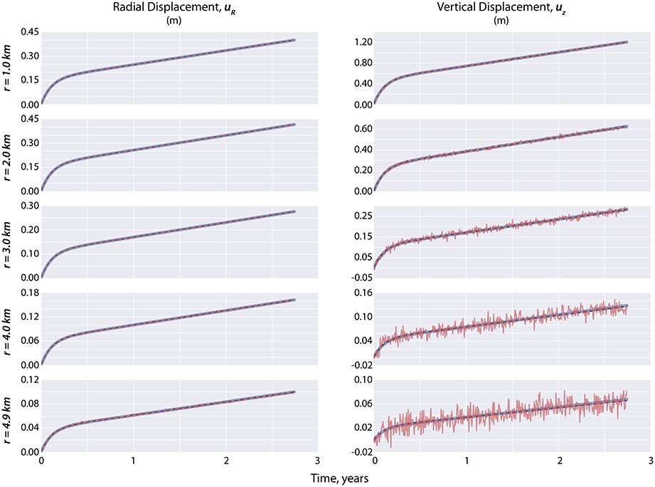
Figure 4. The EnKF-estimated displacements after performing assimilation via state estimation (i.e., blue solid line) given that the prior distribution of the uncertain parameters are close to their true values (Figure 3C). The synthetic displacements used as D during assimilation are the noisy red lines that are more evident in the vertical component at far-field distances. The black broken lines correspond to the true values.
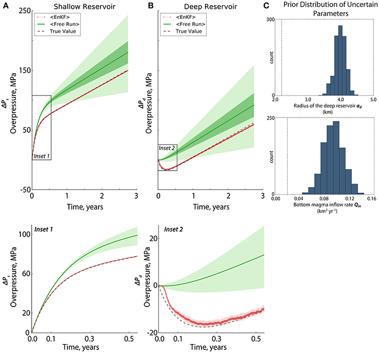
Figure 5. The evolution of the overpressures after performing the state estimation (A,B) given that the initial ensemble of the uncertain parameters (C) are Gaussian, not centered on their true values (black broken lines). The insets provide a magnified image of the overpressures at the beginning of the assimilation. In (A,B) as well as in the insets, the black broken line represents the true value of the overpressures; the green ones represent the result of the free run where the green solid line is the mean, the dark green fill is the spread (1σ) and the light green fill covers the full extent of the ensemble (i.e., [min, max]); the red ones represent the result of EnKF where the red solid line is the mean, the dark red fill is the spread (1σ) and the light red is the full extent of the ensemble. Notice that the spread of the ensemble is very narrow for the assimilation case (~104–106).
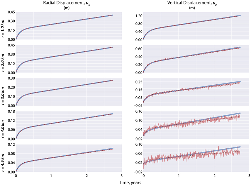
Figure 6. The EnKF-estimated displacements after performing assimilation via state estimation (i.e., blue solid line) given that the prior distribution of the uncertain parameters are far from their true values (Figure 5C). The synthetic displacements used as D during the assimilation are the noisy red lines that are more evident in the vertical component at far-field distances. The black broken lines correspond to the true values.
There are two possible ways to solve the issue in forecasting the displacement: (1) extend the state vector X incorporating the model-forecasted displacements, i.e., , where df = Hxf or (2) extend the state vector incorporating the uncertain parameters (i.e., Equation A4). We opted for the second strategy because it will not only improve the field observation estimates but will also allow us to properly estimate the overpressures and to be able to constrain and gain more knowledge about the uncertain parameters. Furthermore, in performing the first option, the computational cost can increase significantly when we increase the number of observations used during the assimilation, i.e., using InSAR data.
5.2. Synthetic Case B: State-Parameter Estimation
Parameter estimation is very challenging especially when the parameters have no direct link to field observations and if there are no means to compare them to the actual values. The characteristics of the deep magmatic reservoir for example is poorly known in volcanology since it is buried very deep (i.e., >10 km) into the Earth.
We followed the same initial conditions performed in the first case given that: (1) the uncertain parameters are “unbiased” or have truncated-normal distributions, centered on their true values (Figure 3C) and (2) the uncertain parameters are “biased” or have normal distributions but are not centered on their true values (Figure 7C). We used the augmented state vector in Equation (A4) to include the uncertain parameters in the forecasting.
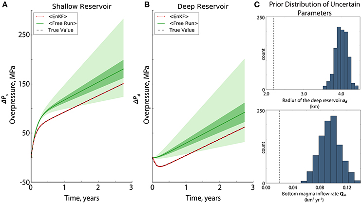
Figure 7. The evolution of the overpressures after performing the state-parameter estimation (A,B) given that the prior distributions of the uncertain parameters (C) are Gaussian, not centered on their true values (black broken lines). In (A,B) the black broken line represents the true value of the overpressures; the green ones represent the result of the free run where the green solid line is the mean overpressure, the dark green fill is the spread (1σ) and the light green fill covers the full extent of the ensemble (i.e., [min, max]); the red ones represent the result of EnKF where the red solid line is the mean, the dark red fill is the spread (1σ) and the light red is the full extent of the ensemble. Notice that the spread of the ensemble is very narrow for the assimilation case.
Results show that the filter tracks almost perfectly the true behavoir of the overpressures given the two different types of parameter initialization as shown for example in Figure 7, where the prior distributions of ad and Qin are biased. In fact, the final values of the overpressures have as little as 0.0−0.01% and 0.04−0.06% error difference with respect to their true values for the shallow and deep overpressures, respectively.
In Figure 8, we plotted ad and Qin at each assimilation step given two different a priori assumptions for the uncertain parameters. Notice how the EnKF-estimated parameters converged well near their true values regardless of how they were initialized. In fact, at the beginning of the assimilation, the filter immediately recognizes its supposed trajectory hence decreases ad and Qin allowing convergence to their true values. Interestingly, we find Qin more sensitive to the estimation than ad as evidenced by the steep drop at the start especially when the prior parameter distribution is biased. To a greater extent, it fell beyond the true value but eventually recuperates and adjusts to its correct behavior. In Table S2 we summarized the results of synthetic case B, showing that there is a very good fit between the EnKF-estimated state variables and model parameters and their true values.
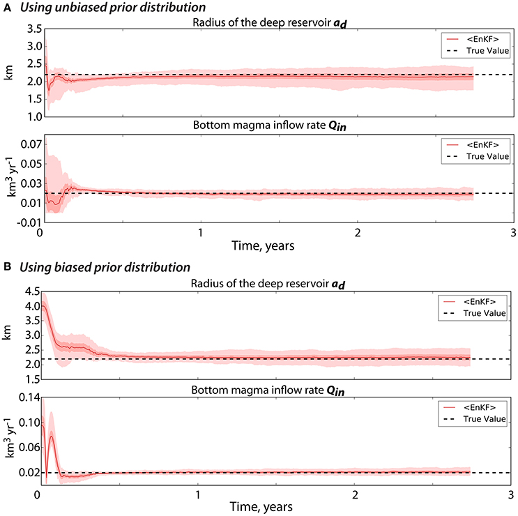
Figure 8. The EnKF-estimated uncertain parameters after performing state-parameter estimation given that the prior distributions of the uncertain parameters are (A) unbiased or (B) biased. The solid red line is the mean value of the uncertain parameters. The dark-shaded red and pink colors represent the spread (1σ) and the [min,max] of the ensemble, respectively. The true values are the black broken lines.
Figure 9 confirms our initial recommendation that augmenting the state vector to include the uncertain parameters in the estimation will correctly forecast the radial and vertical displacements.
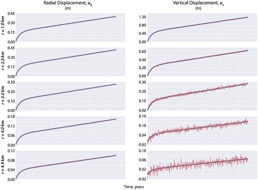
Figure 9. Ten of the 80 EnKF-estimated displacements after performing assimilation via state-parameter estimation (i.e., blue solid line) given that the prior distributions of the parameters are biased (Figure 7C). The synthetic observations used as D during assimilation are the noisy red lines that are more evident in the vertical component at far-field distances. The black broken lines correspond to the true values of the displacements.
6. Discussion
6.1. Influence of Spatial and Temporal Resolutions
6.1.1. High Spatial Resolution vs. High Temporal Resolution Dataset
Our results show the huge potential of EnKF in forecasting the overpressures and displacements as well as in estimating the uncertain model parameters. However, having 40 near-field GNSS stations that will provide 80 observations every 2 days is often not the case for most volcanoes. In Figure 10 we show how EnKF performs when the number of observations is varied using two types of dataset: (1) a GNSS-like dataset and (2) an InSAR-like dataset. The GNSS-like dataset is composed of 10 observations (i.e., five radial and five vertical displacements) located at distance r = 1−5 km away from the volcano axis and is uniformly spaced every 1 km. The InSAR-like data is an 11 × 11 grid centered on zero-axis (i.e., r = 0 as the volcano axis) with two components (i.e., vertical and radial directions) that have spatial resolutions of 1 km. This provides a total of 242 observations located at distance r = 1 to km away from the volcano axis. Each of the datasets is assimilated every 2 days (fobs = 1), consistent with the time interval of the model. We use a prior distribution which is Gaussian and not centered on the true values for the uncertain parameters (Figure 7C) because it is the most realistic and most critical case. Our findings show that both datasets are able to track the true behavior of the shallow and deep overpressures. However, when it comes to estimating the uncertain model parameters, only the InSAR-type data were able to allow convergence of Qin and ad to their true values.
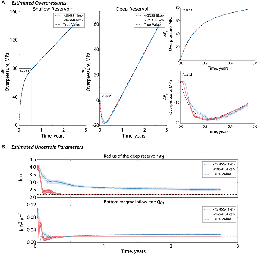
Figure 10. Influence of the spatial density of observations on the assimilation: GNSS (10 observations that are assimilated every time-step, fobs = 1, with distance to the volcanic center ranging from 1 to 5 km) vs. InSAR-like dataset (242 observations that are assimilated every time-step, fobs = 1, with distance to the volcanic center ranging from 1 to km). (A,B) illustrates the estimated overpressures and uncertain parameters, respectively, given that the initial conditions of the uncertain parameters are similar to those of in Figure 5C. The insets in (A) provide a closer look on the overpressures at the beginning of the assimilation. The light blue and red shades correspond to the spreads (1σ). Note that for the overpressures, the spreads are difficult to discern since they are very small when compared to the scale of the plot. The black broken lines represent the true values.
The challenge remains with the availability of InSAR data every 2 days. At the time of writing, only the Sentinel-1 satellite has the capability to provide radar data as frequent as every 6–12 days. TerraSAR-X can provide data every 11 days whereas COSMO SkyMed's routine return period can acquire data every 8 days by using different satellites in its constellation. To be more realistic, we then assimilated the InSAR-like dataset every 12 days (fobs = 1/6) and kept the frequency of available GNSS data to 2 days (fobs = 1). This means that for the InSAR-like data, the model forecasts are only corrected every 12 days. Figure 11 illustrates that the InSAR-like data failed to recover the true behavior of the overpressures toward the end of the assimilation. More precisely, it failed to recover the exponential part of the system or during the time when the shallow reservoir is refilled by the deep one after an eruption. As a consequence of the poor overpressure forecast at the beginning, parameter estimation cannot be performed because their resulting posterior distributions are physically meaningless (i.e., negative radius of the deep reservoir). Performing the resampling option cannot even solve the issue. Take note that in EnKF, uncertain model parameters are only updated by the sample covariance between them and the state variables (i.e., in this case, the overpressures), and that the model evolution for them is simply an identity.
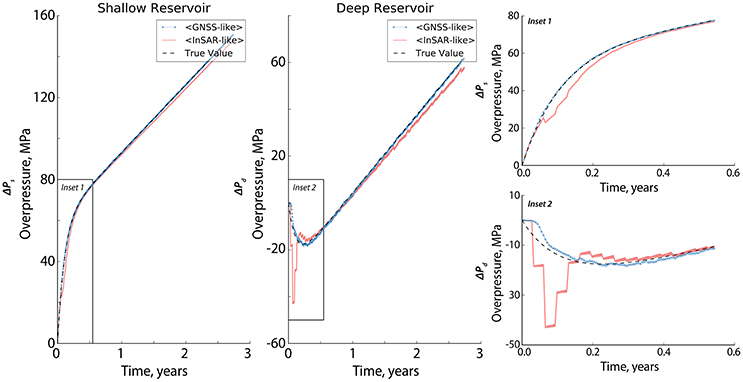
Figure 11. Influence of the frequency of observations on the assimilation: GNSS (10 observations that are assimilated every time step, fobs = 1, with distance to the volcanic center ranging from 1 to 5 km) vs. InSAR-like dataset (242 observations that are assimilated every 12 days, fobs = 1/6, with distance to the volcanic center ranging from 1 to km). Since parameter estimation is not possible to perform when InSAR dataset is used (see text), only the estimated overpressures are presented. Note that the initial conditions of the uncertain parameters are similar to those of in Figure 5C. The insets provide a closer image of the overpressures at the beginning of the assimilation. The light blue and red shades correspond to their spread (1σ). Note that these values are difficult to discern since they are very small when compared to the scale of the plot. The black broken lines represent the true values.
Given the aforementioned results, we know that the advantage of using GNSS data to capture the behavior of the overpressures is its high temporal resolution, in which it is possible to obtain daily observations that can be used for assimilation. InSAR data on the other hand, are less frequent to acquire but provide better spatial information about the surface deformations and constraints on the uncertain parameters. In order to exploit the advantages of both dataset, we jointly assimilated the GNSS-like and InSAR-like data. Figure 12 shows how the evolution of the overpressures is well captured and how the uncertain model parameters converged to their true values. In fact for this case, in as early as ~6 months of jointly assimilating GNSS and InSAR, it may already be possible to forecast the long term overpressure values that can later tell whether a critical overpressure–unique for each volcano–will most likely be achieved.
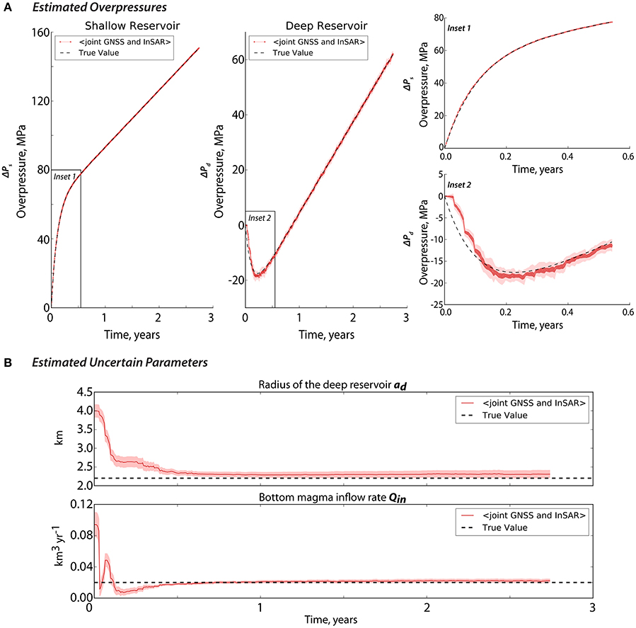
Figure 12. The estimated overpressures (A) and uncertain parameters (B) after jointly assimilating GNSS (10 observations that are assimilated every time-step, fobs = 1, with distance to the volcanic center ranging from 1 to 5 km) and InSAR-like observations (242 observations that are only assimilated every 12 days, fobs = 1/6, with distance to the volcanic center ranging from 1 to km). The initial conditions of the uncertain parameters are similar to those of in Figure 5C. The inset in (A) provides a magnified view of the overpressures at the start of the assimilation. The pink shade corresponds to the spread (1σ). The black broken lines represent the true values.
Retrieving the three-dimensional (3D) displacement vector using InSAR is not always possible and most of the time, only the line-of-sight (LOS) displacement is available. In the Supplementary Materials, we show that the joint assimilation of GNSS and InSAR in either ascending or descending LOS view can still capture the temporal behavior of the overpressures as well as estimate the two uncertain model parameters, thereby allowing the possibility of near-real time forecasting.
6.1.2. Including Far-Field Data
While InSAR data can cover up to hundreds of kilometers with one swath, most volcanoes are small in size and thus volcano deformation signals may cover only a small portion in the image. In Figure S3 we plot the radial and vertical displacements as a function of the distance from the volcano axis given the values of the parameters in Table 1. As one goes farther away from the volcano axis (i.e., r is increased), the deformation signal weakens and almost decays to zero. Decomposing the source of deformation, we find that the near-field signals are mostly related to the shallow reservoir whereas at farther distances (i.e., >16 km and >10 km for the radial and vertical displacements, respectively), the signals became dominated by the deep one. Given this, one can infer that far-field data can bring more information about the deep reservoir but note also that as one goes farther away from the volcano axis, the signal-to-noise ratio also weakens. Thus, when assimilating InSAR data, it is important to know the effect of including far-field data in order to avoid spikes in the root mean square error (RMSE) between the forecasted and the synthetic surface deformation associated with the use of InSAR especially when coupled with GNSS data as previously performed by Gregg and Pettijohn (2016).
To do so, we generated an 11 × 11 grid InSAR-like dataset with two components (i.e., vertical and radial directions), giving a total of 242 data points. However, unlike in the previous section where we assimilate near-field observations that are equally spaced every 1 km, here, we use non-uniform spacing and intentionally limit the number of far-field points to avoid overwhelming the dataset with noise. In Figure 13A, we plotted the location of these observations. Figures 13B,C show the estimated overpressures and the uncertain parameters after assimilating near-field and far-field observations every 2 days. Results show that while the true overpressures are correctly forecasted, the uncertain parameters failed to converge to their true values. In fact, the estimated uncertain parameters worsen when we compare them to the InSAR results in Figure 10 where we only assimilated near-field data. Perturbing the uncertain parameters was not even helpful. Cropping the InSAR data, then downsampling using quadtree (e.g., Simons et al., 2002; Sudhaus and Sigurjón, 2009) and/or placing weights on each pixel may be useful in the future in order to allow strategical assimilation of both near-field and far-field data.
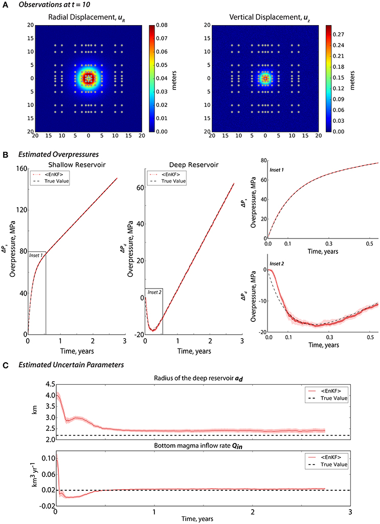
Figure 13. (A) The locations of the 242 observations (i.e., 121 radial and 121 vertical points) in gray dots and their corresponding displacement values at t = 10. The observations are assimilated every time-step such that fobs = 1. Note that the x and y axis are in kilometers. The EnKF-estimated (B) overpressures and (C) uncertain parameters after performing state-parameter estimation using the observations in (A). We used a biased prior distribution for the uncertain parameters like in Figure 5C or Figure 7C. Note that the pink shades represent the spread (1σ) of the estimation. The true values are the black broken lines.
We emphasize that all these discussions are based on specific set of parameters we chose for the synthetic case. In particular, the influence of the spatial and temporal resolution strongly depends on the time constant, τ = 0.11 years and reservoir depths set to 3 and 35 km for the shallow and deep reservoirs, respectively.
6.1.3. Defining the Observation Error Covariance, R
In this study, we added a white Gaussian noise to generate all the observations. This is one of the fundamental assumptions and a common approach in data assimilation that implies the use of diagonal observation error covariance, R, during the computation. Even in many operational weather forecast centers, this simplification is adopted in order to facilitate the implementation on one hand and to ensure the quality of the results on the other hand. In the case of complex data noise, it is usually difficult to precisely characterize the error. Using non-reliable information of observation errors in the computation may worsen the results. Here, we adopted a simple observation error covariance, but in practice, the error variance can be increased in order to take into account the part of error not represented by the error covariance used.
Spatially correlated noise can be present, especially in the case of InSAR data where atmospheric noise are usually embedded in the data. The spatial correlation can change the results depending on the quality, quantity and the distribution of the data points. Bekaert et al. (2016) suggest that neglecting InSAR covariance should be avoided as it may result to treating spatially correlated atmospheric noise as part of the signal. In the future, InSAR variance-covariance shall be applied when dealing with real case data. Furthermore, the approach presented by Brankart et al. (2009) and Ruggiero et al. (2016) can be considered.
6.2. Comparing with Inversion
When performing the comparison between EnKF and inversion, we want to make sure first that the model and the a priori information that we used are the same and are suitable for the two techniques. For example, if we start from a parameter distribution which does not cover the true values of the uncertain parameters (e.g., Figure 5C), the inversion will not work. On the other hand, if we start from a uniform distribution as we used to do in inversion, the EnKF estimation will not be the optimal solution since it requires a prior assumption that is Gaussian in nature. We then built the prior distributions for ad and Qin (Figure 14B) that agrees with the prerequisites of both the assimilation and inversion.
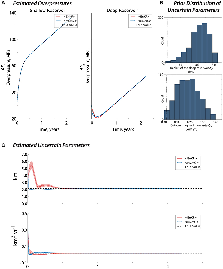
Figure 14. Comparison between the EnKF-estimated and MCMC-estimated (A) overpressures and (C) uncertain model parameters given the prior distributions of ad and Qin in (B). For the two techniques, we used 80 synthetic observations (i.e., combined radial and vertical displacements) located uniformly, every 100 m, at r = 1−4.9 km and are available every time-step. The light blue and pink shades represent the spread (1σ) of the estimation. The true values are the black broken lines.
Gregg and Pettijohn (2016) have previously compared data assimilation with inversion using two different models–a viscoelastic assumption for EnKF and an elastic one for the inversion. In our case, to be fair and consistent, the same forward dynamical model (the two-magma-chamber model) is applied to the two techniques.
For the EnKF, we performed the state-parameter estimation strategy similar to that in synthetic case B. Whereas, we implemented a Bayesian-based estimation, i.e., Markov Chain Monte Carlo (MCMC), for the inversion. MCMC is most useful in cases where models are non-linear and expressing an analytical solution is not possible (Segall, 2013). Note that we used 80 synthetic observations (i.e., 40 radial and 40 vertical displacements) that are uniformly (every 100 m) located at a distance r = 1−4.9 km with frequency of available observation consistent with the time interval (i.e., Δt = 2 days; fobs = 1) for the two techniques.
In performing MCMC, the posterior distribution of the uncertain parameters is sampled given their a priori distribution using the forward model and a proposed likelihood distribution. Models are selected based on the Metropolis-Hastings rules, which always accept models that fit better to observations than the previous iteration and randomly accept those that do not fit to avoid being trapped to a local minima (Segall, 2013). For example, at ti, a set of ad and Qin values are drawn from their initial distributions, generating model forecasts using the two-chamber model. These model forecasts are then compared to the GNSS and/or InSAR data and are always accepted if the fit is better than the last sampling iteration, creating the so-called Markov-Chain. The sampling iteration can be performed thousand to million times in order to build a full posterior distribution. In our case, we performed 11,000 MCMC sampling iterations at each time-step and burned-in the first 10,000 so that in the end we have a similar ensemble size (e.g., 1,000) to that of the EnKF. Take note that unlike in EnKF which is sequential and only uses incoming observations to capture the temporal evolution of the overpressures, MCMC utilizes all the observations from t0 up to the preferred time of observation ti. We performed up to 400 time-steps with interval similar to that in EnKF (i.e., Δt = 2 days).
Figure 14A presents the resulting overpressures after performing EnKF and MCMC. The shallow overpressure is well-estimated by the two approaches, whereas the overpressures in the deep reservoir both started from a deviated value but eventually converged to their true values. The MCMC-estimates are also found smoother than the EnKF-forecasts especially in the deep reservoir. Since EnKF always assumes that the dynamical model is uncertain and needs to be corrected by incoming observations, it then tends to closely follow the behavior of the observations, hence we observe a noisier estimation with EnKF. It follows that MCMC cannot account for epistemic model errors or those uncertainties related to processes not included in the physical forward model (Segall, 2013).
If we observe how the uncertain parameters are estimated by the two techniques in Figure 14C, we will find that both are able to estimate accurately the true values, but MCMC is faster to converge. Take note however, that the uncertain parameters we used in this study are static parameters. In the case of an evolving model parameter, which could be the case for the basal magma inflow (i.e., Poland et al., 2012), the inversion may not be the optimal method to use for estimation.
6.3. Toward More Realistic Physics-Based Models
The model that we used here is a highly simplified view on how a volcano plumbing system works based on idealized assumptions (e.g., elastic medium in a homogeneous half-space, incompressible magma). It can be implemented easily for real-time forecasting of effusive eruptions as contrary to the finite element model of Gregg and Pettijohn (2016). Although we only considered two uncertain model parameters (ad and Qin) in this study, since they are the most difficult to constrain using geodetic data through conventional approach, future work can be extended to explore other parameters such as the depth and the shape of the reservoirs and the strength of the hydraulic connection between them.
In addition to the simplicity and specificity of the model that we tested, we base the potentiality assessment of data assimilation on a synthetic case that is consistent with observations recorded at a specific volcano –Grímsvötn in Iceland. In fact, similar deformation behavior has been observed at other basaltic volcanoes: Kilauea and Mauna Loa in Hawaii (Lengliné et al., 2008, Westdahl Volcano (Lu et al., 2003), and Axial Seamount Volcano (Nooner and Chadwick, 2009) such that it can be accepted as generic for this type of frequently erupting volcanoes. However, except for Axial Seamount, the time constant derived at other places are larger than the one observed at Grímsvötn (Reverso et al., 2014). This parameter is expected to only influence the impact of the temporal frequency of available observations. In the case of Grímsvötn, it is indeed expected to be more restrictive regarding the importance of a high temporal resolution dataset. It was beyond the scope of this first paper to modify the parameters chosen for the synthetic case, but a systematic exploration of the dimensionless parameters will be required in further studies.
We emphasize that the focus of this work is to give a preliminary assessment of how EnKF can be utilized in eruption forecasting rather than validating the dynamical model that we considered. Unlike in the field of ocean-atmosphere science where models are more advanced and established, realistic and generic physics-based models of volcanoes are still in progress. However, one of the main interests in using data assimilation is that it takes into account the fact that models are not perfect and are mostly based on the simplification of the complex reality. This is represented by the model error, q, as depicted in Equation (5). Evensen (2003) have shown that the model error can be accounted in the EnKF scheme using the following expression:
where is the model covariance. represents the accumulated model errors from the beginning of the assimilation until the instant ti+1. In order to overcome the difficulty in quantifying directly the model error at each time-step, the EnKF represents the model error by an ensemble of model state generated from a large number of perturbations of uncertain model parameters. The model error covariance P in the EnKF practice is an approximation of the real model error. In case of infinite ensemble members, P is considered to equal the real model error. For this reason, a large ensemble size is always required. Any dynamical model can actually be used in data assimilation as long as there is a link between the model and the observations and the model can be restarted at any instant. However, take note that models that are too far from the reality would result in large model errors that would be difficult or impossible to correct by the observations, especially when the condition of the observations is not good enough (i.e., in terms of quantity, distribution and accuracy). The use of more realistic physics-based models that could better interpret field observations such as those that could account for magma rheology and compressibility (e.g., Rivalta and Segall, 2008; Anderson and Segall, 2011, 2013; Segall, 2016; Got et al., 2017) are then highly encouraged. Data assimilation can also be extended to models representing other plumbing mechanism such as magma reservoirs recharged by dikes at depth (e.g., Karlstrom et al., 2009) or even those eruptions that are related to dike intrusions.
6.4. Implications to Real-Time Volcano Monitoring
While parameter-estimation allows us to gain more knowledge about the plumbing system and the behavior of the volcano, in real-time crisis, one of the key variables to infer an impending effusive eruption is the overpressure. The EnKF strategy presented here uses a simple dynamical model that can be easily integrated with large amount of real-time geodetic data, allowing to quickly and accurately track the value of the overpressures both in short-term and long-term periods. Assuming a statistic distribution for the threshold magma overpressure leading to reservoir wall rupture, based on previous eruption for instance, the updated overpressure provided by EnKF can be used to estimate the timing of an impending eruption. Although the critical overpressure value is not always known, especially for volcanoes that do not erupt frequently, it depends on the rock strength that can be estimated and on the local stress field strongly influenced by the edifice geometry (Pinel and Jaupart, 2003).
Another important challenge of the assimilation approach is the availability of frequent data. Although for GNSS we can obtain daily observations, InSAR data are less frequent and are still dependent on the quality of interferograms produced. Also, in reality, the 3D-displacement field vector from InSAR are not always retrievable due to the satellite's acquisition geometry. Furthermore, while we only used deformation data alone, the observation vector can include gas emission and seismic data for a more deterministic approach in forecasting (i.e., seismic data in particular can be used to estimate the timing of an eruption), as long as they can be related to the dynamical model used.
Interestingly, when it comes to near-real time monitoring, it may be possible to use inversion and data assimilation jointly in order to accommodate vast amount of incoming data. MCMC allows faster forecasting of non-evolving model parameters whereas EnKF via state-estimation is easy to implement and only requires incoming observations. Meaning, the uncertain model parameters can be first constrained by MCMC and the overpressures will then be forecasted using EnKF via state-estimation strategy (e.g., synthetic case A).
7. Conclusions and Perspectives
Our work presents a simple yet efficient model-data fusion strategy using data assimilation (i.e., EnKF) that can be applied to real-time volcano monitoring. Synthetic GNSS and/or InSAR data are assimilated to a simple yet generic dynamical model (i.e., two-chamber model) to mainly forecast the overpressures–one of the key parameters when assessing volcanic eruptions. The EnKF method is tested on two synthetic cases: (A) state-estimation and (B) state-parameter estimation using different a priori information about the uncertain model parameters. This technique allowed us to provide posterior distributions of the overpressures and the uncertain model parameters at each time step. Our results show that the filter can successfully track the evolution of the overpressures both in the shallow and deep reservoirs using near-field observations if the prior assumptions about the uncertain parameters are well defined or if the uncertain parameters are also estimated along with the state variables (overpressures).
Based on the specific case considered in this study, frequent but spatially sparse observations like GNSS are more likely to recover the true evolution of the overpressures than with an infrequent but spatially dense dataset (e.g., InSAR). Although, using an InSAR-like data will better constrain the uncertain model parameters. While Gregg and Pettijohn (2016) pointed that the assimilation of InSAR creates spikes in the RMSE between the forecasted and the synthetic displacements when coupled with GNSS, our strategy presents a successful joint assimilation of these datasets for the first time, allowing to exploit both the high temporal characteristic of GNSS and the high spatial characteristic of InSAR. An important point to consider is the use of far-field data. While far-field displacements can provide more information about the deep reservoir, they can generate noisier and less accurate forecasts because of their weaker signal-to-noise ratio. Future work must be dedicated to strategically balance them with near-field observations when used for assimilation (i.e., resampling by quadtree and/or imposing weights on the data points). Although, we did not investigate the effect of spatially correlated noise especially in InSAR data, we acknowledge the need to apply InSAR variance-covariance matrix especially in real data as suggested by Bekaert et al. (2016).
The ability of the EnKF and sophisticated Bayesian inversion (MCMC) to constrain parameters of a dynamical model are similar. Both techniques can thus be used to forecast the temporal evolution of magma overpressure through time. Although the use of MCMC allows faster convergence of the uncertain model parameters to their true values, the advantage of data assimilation is clearly to improve the forecasts in near real-time by updating the parameter estimations (thus accounting for the temporal variations of the parameters) based on incoming observations. Interestingly, it may also be possible to combine both techniques in which MCMC will be used to first constrain the non-evolving model parameters followed by applying EnKF in order to forecast only the state variables (e.g., overpressures).
The strategy that we have developed here aims to give a preliminary assessment of EnKF as a tool to assess volcanic unrest. While our framework is simple, it offers a great potential in using the method toward a more deterministic approach in eruption forecasting and better understanding of the magma plumbing system. The use of more sophisticated physics-based models as well as other types of datasets such as gas emission and seismic data are highly encouraged for future studies. In terms of the real case application of the strategy to Grímsvötn volcano, additional uncertain model parameters such as the depth of the deep reservoir and the hydraulic strength between the two reservoirs should be accounted.
Author Contributions
All the authors contributed to the conceptualization and design of the study as well as to the writing of the manuscript. MB: performed the simulations and detailed analyses. VP: contributed to the dynamical model and volcanological point-of-view. YY: contributed mainly to data assimilation.
Conflict of Interest Statement
The authors declare that the research was conducted in the absence of any commercial or financial relationships that could be construed as a potential conflict of interest.
The reviewer GMC and handling Editor declared their shared affiliation, and the handling Editor states that the process nevertheless met the standards of a fair and objective review.
Acknowledgments
The authors would like to thank Dr. Bernard Valette and Dr. Jean-Michel Brankart for their helpful discussions about the inversion method and data assimilation, respectively. We are also grateful for the scientific comments of Dr. Marie-Pierre Doin and Dr. Jean-Luc Froger. Furthermore, we also acknowledge our two reviewers and Dr. Valerio Acocella for their constructive comments that helped to improve our work.
Supplementary Material
The Supplementary Material for this article can be found online at: https://www.frontiersin.org/article/10.3389/feart.2017.00048/full#supplementary-material
References
Alfaro, R., Brandsdóttir, B., Rowlands, D. P., White, R. S., and Gudmundsson, M. T. (2007). Structure of the Grímsvötn central volcano under the Vatnajökull icecap, Iceland. Geophys. J. Int. 168, 863–876. doi: 10.1111/j.1365-246X.2006.03238.x
Anderson, K., and Segall, P. (2011). Physics-based models of ground deformation and extrusion rate at effusively erupting volcanoes. J. Geophys. Res. Solid Earth 116:B07204. doi: 10.1029/2010jb007939
Anderson, K., and Segall, P. (2013). Bayesian inversion of data from effusive volcanic eruptions using physics-based models: application to Mount St. Helens 2004–2008. J. Geophys. Res. Solid Earth 118, 2017–2037. doi: 10.1002/jgrb.50169
Aoki, Y., Segall, P., Kato, T., Cervelli, P., and Shimada, S. (1999). Imaging magma transport during the 1997 seismic swarm off the Izu Peninsula, Japan. Science 286, 927–930. doi: 10.1126/science.286.5441.927
Auriac, A., Sigmundsson, F., Hooper, A., Spaans, K. H., Björnsson, H., Pálsson, F., et al. (2014). InSAR observations and models of crustal deformation due to a glacial surge in Iceland. Geophys. J. Int. 198, 1329–1341. doi: 10.1093/gji/ggu205
Bagnardi, M., and Amelung, F. (2012). Space-geodetic evidence for multiple magma reservoirs and subvolcanic lateral intrusions at Fernandina Volcano, Galápagos Islands. J. Geophys. Res. Solid Earth 117:B10406. doi: 10.1029/2012JB009465
Barbu, A., Calvet, J.-C., Mahfouf, J.-F., Albergel, C., and Lafont, S. (2011). Assimilation of soil wetness index and leaf area index into the ISBA-A-gs land surface model: grassland case study. Biogeosciences 8, 1971–1986. doi: 10.5194/bg-8-1971-2011
Bartlow, N. M., Wallace, L. M., Beavan, R. J., Bannister, S., and Segall, P. (2014). Time-dependent modeling of slow slip events and associated seismicity and tremor at the Hikurangi subduction zone, New Zealand. J. Geophys. Res. Solid Earth 119, 734–753. doi: 10.1002/2013JB010609
Bekaert, D., Segall, P., Wright, T., and Hooper, A. (2016). A network inversion filter combining GNSS and InSAR for tectonic slip modeling. J. Geophys. Res. Solid Earth. 121, 2069–2086. doi: 10.1002/2015jb012638
Brankart, J.-M., Ubelmann, C., Testut, C.-E., Cosme, E., Brasseur, P., and Verron, J. (2009). Efficient parameterization of the observation error covariance matrix for square root or ensemble kalman filters: application to ocean altimetry. Month. Weather Rev. 137, 1908–1927. doi: 10.1175/2008MWR2693.1
Burgers, G., Jan van Leeuwen, P., and Evensen, G. (1998). Analysis scheme in the ensemble Kalman filter. Month. Weather Rev. 126, 1719–1724.
Carrier, A., Got, J.-L., Peltier, A., Ferrazzini, V., Staudacher, T., Kowalski, P., et al. (2014). A damage model for volcanic edifices: implications for edifice strength, magma pressure, and eruptive processes Special Section. J. Geophys. Res. Solid Earth 120, 567–583. doi: 10.1002/2014JB011485
Chadwick, W. W., Jónsson, S., Geist, D. J., Poland, M., Johnson, D. J., Batt, S., et al. (2011). The may 2005 eruption of fernandina volcano, galápagos: the first circumferential dike intrusion observed by GPS and insar. Bull. Volcanol. 73, 679–697. doi: 10.1007/s00445-010-0433-0
Chen, Y., and Oliver, D. S. (2010). Ensemble-based closed-loop optimization applied to Brugge field. SPE Reserv. Eval. Eng. 13, 56–71. doi: 10.2118/118926-PA
Elsworth, D., Mattioli, G., Taron, J., Voight, B., and Herd, R. (2008). Implications of magma transfer between multiple reservoirs on eruption cycling. Science 322, 246–248. doi: 10.1126/science.1161297
Evensen, G. (1994). Sequential data assimilation with a nonlinear quasi-geostrophic model using Monte Carlo methods to forecast error statistics. J. Geophys. Res. 99, 10143–10162. doi: 10.1029/94JC00572
Evensen, G. (2003). The ensemble Kalman Filter: theoretical formulation and practical implementation. Ocean Dyn. 53, 343–367. doi: 10.1007/s10236-003-0036-9
Evensen, G. (2009). Data Assimilation: The Ensemble Kalman Filter. Berlin: Springer Science & Business Media.
Fournier, A., Eymin, C., and Alboussiere, T. (2007). A case for variational geomagnetic data assimilation: insights from a one-dimensional, nonlinear, and sparsely observed mhd system. Nonlin. Processes Geophys. 14, 163–180. doi: 10.5194/npg-14-163-2007
Fournier, A., Hulot, G., Jault, D., Kuang, W., Tangborn, A., Gillet, N., et al. (2010). An introduction to data assimilation and predictability in geomagnetism. Space Sci. Rev. 155, 247–291. doi: 10.1007/s11214-010-9669-4
Fournier, T., Freymueller, J., and Cervelli, P. (2009). Tracking magma volume recovery at Okmok volcano using GPS and an unscented Kalman filter. J. Geophys. Res. Solid Earth 114:B02405. doi: 10.1029/2008jb005837
Geir, N., Johnsen, L. M., Aanonsen, S. I., and Vefring, E. H. (2003). “Reservoir monitoring and continuous model updating using ensemble Kalman filter,” in SPE Annual Technical Conference and Exhibition (Denver: Society of Petroleum Engineers).
Geirsson, H., LaFemina, P., Arnadottir, T., Sturkell, E., Sigmundsson, F., Travis, M., et al. (2012). Volcano deformation at active plate boundaries: deep magma accumulation at Hekla volcano and plate boundary deformation in south Iceland. J. Geophys. Res. Solid Earth 117:B11409. doi: 10.1029/2012jb009400
Gillet, N., Barrois, O., and Finlay, C. C. (2015). Stochastic forecasting of the geomagnetic field from the COV-OBS. X1 geomagnetic field model, and candidate models for IGRF-12. Earth Planets Space 67:71. doi: 10.1186/s40623-015-0225-z
Got, J.-L., Carrier, A., Marsan, D., Jouanne, F., Vogfjörd, K., and Villemin, T. (2017). An Analysis of the non-linear magma-edifice coupling at Grimsvötn volcano (Iceland). J. Geophys. Res. Solid Earth 122, 826–843. doi: 10.1002/2016JB012905
Gregg, P. M., and Pettijohn, J. C. (2016). A multi-data stream assimilation framework for the assessment of volcanic unrest. J. Volcanol. Geothermal Res. 309, 63–77. doi: 10.1016/j.jvolgeores.2015.11.008
Grewal, M. S., and Andrews, A. P. (2008) Practical Considerations, in Kalman Filtering, 3rd Edn. Hoboken, NJ: John Wiley & Sons, Inc. doi: 10.1002/9780470377819.ch8
Gu, Y., and Oliver, D. S. (2005). History matching of the punq-s3 reservoir model using the ensemble Kalman filter. SPE J. 10, 217–224. doi: 10.2118/89942-PA
Hautmann, S., Witham, F., Christopher, T., Cole, P., Linde, A. T., Sacks, I. S., et al. (2014). Strain field analysis on montserrat (wi) as tool for assessing permeable flow paths in the magmatic system of soufrière hills volcano. Geochem. Geophys. Geosyst. 15, 676–690. doi: 10.1002/2013GC005087
Houtekamer, P. L., and Mitchell, H. L. (2005). Ensemble kalman filtering. Q. J. R. Meteorol. Soc. 131, 3269–3289. doi: 10.1256/qj.05.135
Hreinsdóttir, S., Sigmundsson, F., Roberts, M. J., Björnsson, H., Grapenthin, R., Arason, P., et al. (2014). Volcanic plume height correlated with magma-pressure change at Grimsvotn Volcano, Iceland. Nat. Geosci. 7, 214–218. doi: 10.1038/ngeo2044
Julier, S. J., and Uhlmann, J. K. (2004). Unscented filtering and nonlinear estimation. Proc. IEEE 92, 401–422. doi: 10.1109/JPROC.2003.823141
Kalman, R. E. (1960). A new approach to linear filtering and prediction problems. J. Basic Eng. 82, 35–45. doi: 10.1115/1.3662552
Karlstrom, L., Dufek, J., and Manga, M. (2009). Organization of volcanic plumbing through magmatic lensing by magma chambers and volcanic loads. J. Geophys. Res. Solid Earth 114:B10204. doi: 10.1029/2009jb006339
Kuang, W., Wei, Z., Holme, R., and Tangborn, A. (2010). Prediction of geomagnetic field with data assimilation: a candidate secular variation model for IGRF-11. Earth Planets Space 62, 775–785. doi: 10.5047/eps.2010.07.008
Lengliné, O., Marsan, D., Got, J. L., Pinel, V., Ferrazzini, V., and Okubo, P. G. (2008). Seismicity and deformation induced by magma accumulation at three basaltic volcanoes. J. Geophys. Res. Solid Earth 113, 1–12. doi: 10.1029/2008jb005937
Lorentzen, R. J., Fjelde, K. K., Frøyen, J., Lage, A. C., Nævdal, G., Vefring, E. H., et al. (2001). “Underbalanced and low-head drilling operations: real time interpretation of measured data and operational support,” in SPE Annual Technical Conference and Exhibition (Amsterdam: Society of Petroleum Engineers).
Lu, Z., Masterlark, T., Dzurisin, D., Rykhus, R., and Wicks, C. (2003). Magma supply dynamics at westdahl volcano, alaska, modeled from satellite radar interferometry. J. Geophys. Res. Solid Earth 108:2354. doi: 10.1029/2002jb002311
McGuire, J. J., and Segall, P. (2003). Imaging of aseismic fault slip transients recorded by dense geodetic networks. Geophys. J. Int. 155, 778–788. doi: 10.1111/j.1365-246X.2003.02022.x
McTigue, D. (1987). Elastic stress and deformation near a finite spherical magma body: resolution of the point source paradox. J. Geophys. Res. Solid Earth 92, 12931–12940. doi: 10.1029/JB092iB12p12931
Mogi, K. (1958). Relations between the eruptions of various volcanoes and the deformations of the ground surfaces around them. Bull. Earthquake Res. Inst. Univ. Tokyo 36, 99–134.
Nooner, S. L., and Chadwick, W. W. (2009). Volcanic inflation measured in the caldera of Axial Seamount: implications for magma supply and future eruptions. Geochem. Geophys. Geosyst. 10:Q02002. doi: 10.1029/2008gc002315
Peltier, A., Beauducel, F., Villeneuve, N., Ferrazzini, V., Di Muro, A., Aiuppa, A., et al. (2016). Deep fluid transfer evidenced by surface deformation during the 2014–2015 unrest at Piton de la Fournaise volcano. J. Volcanol. Geothermal Res. 321, 140–148. doi: 10.1016/j.jvolgeores.2016.04.031
Pinel, V., and Jaupart, C. (2003). Magma chamber behavior beneath a volcanic edifice. J. Geophys. Res. Solid Earth 108:2072. doi: 10.1029/2002jb001751
Pinel, V., Jaupart, C., and Albino, F. (2010). On the relationship between cycles of eruptive activity and growth of a volcanic edifice. J. Volcanol. Geothermal Res. 194, 150–164. doi: 10.1016/j.jvolgeores.2010.05.006
Pinel, V., Poland, M. P., and Hooper, A. (2014). Volcanology: lessons learned from synthetic aperture radar imagery. J. Volcanol. Geothermal Res. 289, 81–113. doi: 10.1016/j.jvolgeores.2014.10.010
Poland, M. P., Miklius, A., Sutton, A. J., and Thornber, C. R. (2012). A mantle-driven surge in magma supply to Kilauea Volcano during 2003–2007. Nat. Geosci. 5, 295–300. doi: 10.1038/ngeo1426
Reichle, R. H., Koster, R. D., Liu, P., Mahanama, S. P., Njoku, E. G., and Owe, M. (2007). Comparison and assimilation of global soil moisture retrievals from the Advanced Microwave Scanning Radiometer for the Earth Observing System (AMSR-E) and the Scanning Multichannel Microwave Radiometer (SMMR). J. Geophys. Res. Atmospheres 112:D09108. doi: 10.1029/2006jd008033
Reverso, T., Vandemeulebrouck, J., Jouanne, F., Pinel, V., Villemin, T., Sturkell, E., et al. (2014). A two-magma chamber model as a source of deformation at Grímsvötn Volcano, Iceland. J. Geophys. Res. Solid Earth 119, 4666–4683. doi: 10.1002/2013JB010569
Rivalta, E., and Segall, P. (2008). Magma compressibility and the missing source for some dike intrusions. Geophys. Res. Lett. 35:L04306. doi: 10.1029/2007gl032521
Roult, G., Peltier, A., Taisne, B., Staudacher, T., Ferrazzini, V., Di Muro, A., et al. (2012). A new comprehensive classification of the Piton de la Fournaise activity spanning the 1985–2010 period. Search and analysis of short-term precursors from a broad-band seismological station. J. Volcanol. Geothermal Res. 241, 78–104. doi: 10.1016/j.jvolgeores.2012.06.012
Ruggiero, G. A., Cosme, E., Brankart, J.-M., Le Sommer, J., and Ubelmann, C. (2016). An efficient way to account for observation error correlations in the assimilation of data from the future swot high-resolution altimeter mission. J. Atmospher. Ocean. Technol. 33, 2755–2768. doi: 10.1175/JTECH-D-16-0048.1
Segall, P. (2013). Volcano deformation and eruption forecasting. Geol. Soc. Lond. 380, 85–106. doi: 10.1144/SP380.4
Segall, P. (2016). Repressurization following eruption from a magma chamber with a viscoelastic aureole. J. Geophys. Res. Solid Earth 121, 8501–8522. doi: 10.1002/2016jb013597
Segall, P., and Matthews, M. (1997). Time dependent inversion of geodetic data. J. Geophys. Res. 102, 22–391. doi: 10.1029/97JB01795
Shirzaei, M., and Walter, T. (2010). Time-dependent volcano source monitoring using interferometric synthetic aperture radar time series: a combined genetic algorithm and Kalman filter approach. J. Geophys. Res. Solid Earth 115:B10421. doi: 10.1029/2010jb007476
Sigmundsson, F., Hooper, A., Hreinsdóttir, S., Vogfjörd, K. S., Ófeigsson, B. G., Heimisson, E. R., et al. (2015). Segmented lateral dyke growth in a rifting event at Bardarbunga volcanic system, Iceland. Nature 517, 191–195. doi: 10.1038/nature14111
Simons, M., Fialko, Y., and Rivera, L. (2002). Coseismic deformation from the 1999 Mw 7.1 Hector Mine, California, earthquake as inferred from InSAR and GPS observations. Bull. Seismol. Soc. Am. 92, 1390–1402. doi: 10.1785/0120000933
Sudhaus, H., and Sigurjón, J. (2009). Improved source modelling through combined use of insar and gps under consideration of correlated data errors: application to the june 2000 kleifarvatn earthquake, iceland. Geophys. J. Int. 176, 389–404. doi: 10.1111/j.1365-246X.2008.03989.x
Swanson, D., Casadevall, T., Dzurisin, D., Malone, S., Newhall, C., and Weaver, C. (1983). Predicting eruptions at Mount St. Helens, June 1980 through December 1982. Science 221, 1369–1376. doi: 10.1126/science.221.4618.1369
Talagrand, O. (1997). Assimilation of observations, an introduction. J. Meteorol. Soc. Japan II 75, 191–209. doi: 10.2151/jmsj1965.75.1B_191
Talagrand, O., and Courtier, P. (1987). Variational assimilation of meteorological observations with the adjoint vorticity equation. I: theory. Q. J. R. Meteorol. Soc. 113, 1311–1328. doi: 10.1002/qj.49711347812
Tiampo, K. F., González, P. J., Samsonov, S., Fernández, J., and Camacho, A. (in press). Principal component analysis of msbas dinsar time series from Campi flegrei, Italy. J. Volcanol. Geothermal Res. doi: 10.1016/j.jvolgeores.2017.03.004
Voight, B., Hoblitt, R., Clarke, A., Lockhart, A., Miller, A., Lynch, L., et al. (1998). Remarkable cyclic ground deformation monitored in real-time on Montserrat, and its use in eruption forecasting. Geophys. Res. Lett. 25, 3405–3408. doi: 10.1029/98GL01160
Yan, Y., Barth, A., and Beckers, J.-M. (2014). Comparison of different assimilation schemes in a sequential Kalman filter assimilation system. Ocean Model. 73, 123–137. doi: 10.1016/j.ocemod.2013.11.002
Zoccarato, C., Baù, D., Ferronato, M., Gambolati, G., Alzraiee, A., and Teatini, P. (2016). Data assimilation of surface displacements to improve geomechanical parameters of gas storage reservoirs. J. Geophys. Res. Solid Earth 121, 1441–1461. doi: 10.1002/2015jb012090
Appendix
A. The Overpressures as State Variables
The state vector, X, can be expressed as:
where ΔPs is the overpressure in the shallow reservoir and ΔPd is the overpressure in the deep reservoir.
From Equations (1) and (2), if we let, , A1 = (ρr − ρm)gHc, and , then we can write the dynamical model as:
where the model operator, .
The relationships of the surface displacements and the overpressures are described by Equations (3) and (4), if we let , and , then we can rewrite them into a matrix of the form:
where the observation vector, and the observation operator, . Note that r are the GNSS locations of the observations (i.e., distance at the surface to the center of the volcanic system) and, Hs and Hd are the depths of the shallow and deep reservoirs, respectively (see Figure 1). The observation error covariance, , in which σuR and σuz are the typical GNSS instrument error values equal to 1 and 10 mm, respectively.
B. The Overpressures and the Uncertain Parameters in the State Vector
Let the state vector be expressed as:
where ΔPs is the overpressure in the shallow reservoir, ΔPd is the overpressure in the deep reservoir, ad is the radius of the deep reservoir and Qin is the basal magma inflow rate. We rewrite the dynamical model into matrix form, i.e.,
such that the model operator is now . On the other hand, D and R will stay the same but the observation operator needs to be modified in order to be consistent with the equations. Hence, it should take the form, .
Keywords: data assimilation, Ensemble Kalman Filter, eruption forecasting, InSAR, GNSS, volcano deformation
Citation: Bato MG, Pinel V and Yan Y (2017) Assimilation of Deformation Data for Eruption Forecasting: Potentiality Assessment Based on Synthetic Cases. Front. Earth Sci. 5:48. doi: 10.3389/feart.2017.00048
Received: 31 January 2017; Accepted: 29 May 2017;
Published: 28 June 2017.
Edited by:
Jacopo Selva, Istituto Nazionale di Geofisica e Vulcanologia, ItalyReviewed by:
Gilda Maria Currenti, Istituto Nazionale di Geofisica e Vulcanologia, ItalyMatt Pritchard, Cornell University, United States
Copyright © 2017 Bato, Pinel and Yan. This is an open-access article distributed under the terms of the Creative Commons Attribution License (CC BY). The use, distribution or reproduction in other forums is permitted, provided the original author(s) or licensor are credited and that the original publication in this journal is cited, in accordance with accepted academic practice. No use, distribution or reproduction is permitted which does not comply with these terms.
*Correspondence: M. Grace Bato, Grace.Bato@univ-smb.fr