


Abstract
A method for combining the asymptotic operator designed by Beylkin (Born migration operator) for the solution of linearized inverse problems with full waveform inversion is presented. This operator is used to modify the standard L2 norm that measures the distance between synthetic and observed data. The modified misfit function measures the discrepancy of the synthetic and observed data after they have been migrated using the Beylkin operator. The gradient of this new misfit function is equal to the cross-correlation of the single scattering data with migrated/demigrated residuals. The modified misfit function possesses a Hessian operator that tends asymptotically towards the identity operator. The trade-offs between discrete parameters are thus reduced in this inversion scheme. Results on 2-D synthetic case studies demonstrate the fast convergence of this inversion method in a migration regime. From an accurate estimation of the initial velocity, three and five iterations only are required to generate high-resolution P-wave velocity estimation models on the Marmousi 2 and synthetic Valhall case studies.
1 INTRODUCTION
Full Waveform Inversion (FWI) has reached today sufficient maturity for being routinely included in the industrial seismic imaging workflow. The method is based on the iterative minimization of the misfit between recorded and synthetic seismograms. The synthetic seismograms are computed through the solution of partial differential equations describing the seismic wave propagation. The minimization of the misfit function is performed over a set of parameters of these equations, which control the wave propagation. This simple formalism allows one to quantitatively estimate physical parameters such as P- and S-wave velocities, density, attenuation and anisotropy coefficients, with a resolution of the order of the wavelength.
Appearing in the early work of Lailly (1983) and Tarantola (1984), FWI was initially thought of as intractable for realistic applications. At that time, the lack of long offsets and low frequencies in the recorded seismic data were responsible for a large gap between the low and high part of the spatial spectrum (wavenumber) which could be reconstructed (Jannane et al.1989). Besides, the computational cost of the method was seen as a major limitation (Gauthier et al.1986).
The simultaneous development of wide-aperture broadband acquisition systems and high-performance computing facilities during the last three decades allowed for the successful application of FWI to real data in the 2-D acoustic and elastic approximations (Operto et al.2004, 2006; Ravaut et al.2004; Gao et al.2006; Brossier et al.2009; Prieux et al.2011; Plessix et al.2012; Prieux et al.2013a,b) as well as in the 3-D acoustic approximation (Sirgue et al.2008; Plessix & Perkins 2010; Vigh et al.2010; Warner et al.2013). An overview of the FWI method and its application to synthetic and real case study data has been proposed by Virieux & Operto (2009).
The two key ingredients involved in the FWI process are first- and second-order derivatives of the misfit function, namely the gradient and the Hessian operators. These ingredients are used at each iteration to construct the update that corrects the current subsurface model estimation. The gradient is built as the cross-correlation of the data residuals with the signals that would be scattered by localized perturbations missing in the initial subsurface model. In this sense, the model update provided by the gradient is an interpretation of the unexplained part of the seismograms (the residuals) in terms of single scattering effects. However, the gradient does not contain any information about the true amplitude of the missing perturbations, and the single scattering assumption is violated as soon as multiscattered arrivals have been recorded. In addition, when multiple classes of parameters are involved in the reconstruction process, trade-offs are expected as the signal scattered by a local perturbation of one parameter class may resemble the signal scattered by a perturbation of another parameter class. A review of these difficulties, especially in the multiparameter inversion framework, is given in Operto et al. (2013) and Alkhalifah & Plessix (2014).
Better accounting for the influence of the Hessian operator in the inversion process should help to mitigate these difficulties. Since the pioneering work of Pratt et al. (1998), numerous studies have been proposed on effects of the inverse Hessian operator. Applying this operator to the gradient restores the amplitude of the perturbations and corrects for artefacts generated by second-order reflections. In addition, it helps refocus the model update and mitigates the trade-offs between parameter classes, as the Hessian operator accounts for spatial and parameter trade-offs.
These well-identified properties have led the FWI community to improve the Hessian operator approximation in the inversion schemes, progressively going from pre-conditioned steepest descent using diagonal approximations of the Gauss–Newton operator (Operto et al.2004) or of the pseudo-Hessian operator (Shin et al.2001), to non-linear conjugate gradient methods (Fichtner et al.2008), l-BFGS approximations (Brossier et al.2009) and truncated Newton methods (Métivier et al.2013, 2014; Castellanos et al.2015). The latter method is based on an approximate solution of the linear system associated with the Newton equations. This approximate solution is computed through few iterations of a linear conjugate gradient solver. This only requires the ability to compute efficiently the action of the Hessian operator on a given vector (matrix-free paradigm). This operation requires two additional solutions of the forward problem using second-order adjoint methods (Métivier et al.2012).
Despite the importance of the inverse Hessian operator in FWI, the aforementioned techniques still rely on a quite crude approximation of this operator. Diagonal Gauss–Newton and pseudo-Hessian approaches only account for the diagonal elements. Few gradients (from 3 to 20 in practice) are used to construct the l-BFGS approximation. The number of internal iterations involved in the solution of the Newton equations should not exceed 10–20 for the truncated Newton method to remain computationally feasible. These numbers have to be compared to the actual size of the Hessian operator in realistic applications: after discretization, the Hessian operator is a square matrix of size N = O(106) in 2-D and N = O(109) in 3-D. The imperfect illumination of the subsurface causes this matrix to be poorly conditioned, making difficult to approximate the solution of the Newton equations in such a small number of iterations.
In this study, an alternative approach is investigated. The underlying idea is to consider a modification of the standard FWI misfit function that yields a misfit function with a Hessian operator tending asymptotically towards the identity. The minimization of this modified misfit function is a better conditioned problem compared to the original one. In particular, in the domain of validity of this modified misfit function, the trade-offs between parameters should be reduced.
The modification of the misfit function consists in projecting the observed and synthetic data on the model space, through a migration operator. The misfit function is thus computed as the L2 norm of residuals in the model space, instead of being defined in the data space. The migration operator that is used is the one proposed by Beylkin & Burridge (1990), developed in the framework of inversion as an approximate inverse of the Born modelling operator (Beylkin 1985, 1987; Bleistein et al.1985; Bleistein 1987; Beylkin & Burridge 1990; ten Kroode 2012).
The dominant part of the Hessian operator of the modified misfit function (the Gauss–Newton part) is a normal operator associated with a modified Born modelling operator. As a result of the introduction of the migration operator in the misfit function, this modified Born modelling operator matrix is equal to the Born modelling operator left-multiplied by the Beylkin operator. This operator tends asymptotically towards the identity. As a consequence, the normal operator associated with this modified Born operator tends asymptotically towards the identity.
A first attempt to use the Beylkin operator in the framework of least-squares inversion has been proposed by Jin (1992), merging two apparent disconnected methods. The underlying idea was to introduce the asymptotic inverse in the misfit function as a data weighting operator to produce a modified misfit function with a nearly diagonal Hessian operator. Unfortunately, as the weighting operator is a mapping from the data space to the model space, the resulting misfit function depends on the space location, which prevents the use of standard non-linear optimization techniques. A similar idea has also been exploited by Sevink & Herman (1996) for accelerating the solution of a least-squares migration problem.
The strategy proposed here may be interpreted as applying a migration algorithm to the data residuals, meaning that the modelled and the recorded data are compared in the migrated (spatial) domain. This shares some similarities with the Differential Semblance Optimization (DSO) methods introduced by Symes & Carazzone (1991) as a particular Migration Velocity Analysis (MVA) method (Symes 2008). In these methods, however, the philosophy is different. The data are migrated using a particular background velocity model in an extended model space. The quality of the background velocity model is assessed using a semblance criterion defined in this extended image domain (invariance along the offset for instance). This semblance criterion is used to define a new misfit function in the extended image domain, and the background velocity model is updated to reduce this misfit.
In the method presented in this study, the velocity model used to perform the migration is kept constant, equal to the initial guess, throughout the iteration process. The migration of the data residuals could be interpreted as a change of metric for comparing synthetic and observed data. The residuals are projected in the model space along the geodesics defined by selected ray paths. The minimization is performed to fit the converted data in this new space, and the migration is not used to assess the quality of the background model. The quality of this model may be poor: in this case the asymptotic approximation of the Hessian operator will be far from the identity operator. However, throughout the iterative process, FWI may still allow to correct the subsurface model that is inverted.
In Section 2, the main ideas from the work of Beylkin (1985), leading to the definition of an approximate inverse of the Born operator, are exposed. The Section 3 presents how the asymptotic migration operator is used within this context to modify the FWI misfit function yielding a better conditioned minimization problem. Numerical experiments on synthetic case studies are presented in Section 4 in a 2-D acoustic frequency-domain context for the reconstruction of the pressure wave velocity only (mono-parameter inversion). The advantages and the limits of the approach are presented. The introduction of the Beylkin operator within the misfit function acts as a scattering-angle-based filtering on the seismic data. A stronger weight is given to reflection data, detrimental to data associated with diving waves. This hampers the reconstruction of the long wavelength of the models. On the other hand, starting from an accurate initial velocity model, the gain in convergence speed is substantial. This study thus suggests that the method presented here may be well suited in a quantitative migration context, for the reconstruction of high-resolution estimates of the subsurface parameters, as it is the case for instance in Métivier (2011) and Métivier et al. (2011). In addition, it shows that far from the high-frequency regime, the asymptotic approximation has still a significant effect on the conditioning of the FWI problem.
2 LINEARIZED SEISMIC INVERSE PROBLEM
2.1 Definitions and notations
2.2 Linearized inversion
Use the first-order Born approximation to derive an analytic expression for J(m0) depending on the Green functions G0(x, ω, xs) and G0(x, ω, xr) associated with eq. (2).
Compute an asymptotic approximation of J(m0), denoted by |$\scr {J}(m_0)$|, through the asymptotic approximation of the Green functions G0(x, ω, xs) and G0(x, ω, xr).
Compute an approximate left inverse of |$\scr {J}(m_0)$|, denoted by |$\scr {B}(m_0)$|. The latter operator is roughly equivalent to a preserved-amplitude migration operator.
2.3 First-order Born approximation
2.4 Asymptotic approximation: computation of |$\scr {J}(m_0)$|
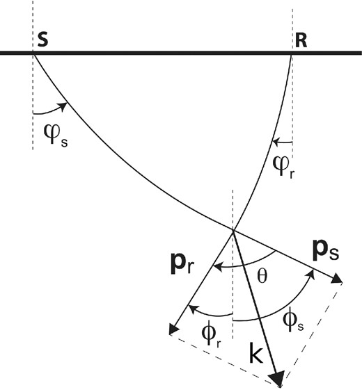
Angles ϕr(xr, x), ϕs(xs, x) and θ(xr, x, xs) for a given source–receiver pair.
2.5 Computation of |$\scr {B}(m_0)$|
The build-up of the operator |$\scr {B}$| is thus an approximate left inverse to the linear operator |$\scr {J}$|. The explicit computation of the operator |$\scr {B}$| is presented in Appendix B in the 2-D mono-parameter case.
3 MODIFICATION OF THE STANDARD FWI MISFIT FUNCTION
3.1 The FWI problem
3.2 Link with the linearized inverse problem
The connection with the linearized inversion can be made here. Eq. (54) is similar to the linearized inverse problem (10), where Δm0 is replaced by δm. These two model updates are two approximate solutions of the same problem. They differ in the approximation used to compute them. In the linearized inverse method proposed by Beylkin, the preserved-amplitude migration operator |$\scr {B}(m_0)$| is used. In the context of the Gauss–Newton method, the solution of this equation in the least-squares sense is computed numerically .
3.3 Introducing the asymptotic inverse within the FWI process
The idea introduced by Jin (1992) is to add a proper scaling in the definition of the associated misfit function, so that the Hessian of this new misfit function should be close from the identity in the asymptotic regime. The scaling acts on the data and corresponds to a weighting function Q(x, xr, xs, ω) derived from the one introduced by Beylkin in its definition of the asymptotic inverse of the linearized forward operator. However, since the weighting Q(x, xr, xs, ω) depends on the space variable |$x \in \mathbb {R}^{n}$|, the resulting misfit function actually depends on the space variable x. This raises substantial difficulties, as for numerical optimization methods to be used, the misfit function should be positive and scalar-valued.
The definition of g(m) given in eq. (56) assumes implicitly that the pre-conditioning operator |$\scr {B}(m_0)$| is computed once for all in the initial model m0. In fact, one may select a suitable model mb as the background model where the pre-conditioning operator |$\scr {B}(m_{\rm b})$| is built. Of course, a more elaborate strategy could consist in introducing another non-linearity in g(m) by letting the pre-conditioning operator depend on the current subsurface model m through an updated background model. However, this brings an additional complexity to the problem, not only in terms of computational effort but also in terms of optimization strategy, as the computation of the gradient of g(m) should be modified accordingly. This study is thus restricted to the case where the pre-conditioning operator is computed in the initial model m0.
4 NUMERICAL STUDY
4.1 Experimental settings and implementation
The aim of the three experiments proposed in this section is to compare standard L2 norm-based FWI results with the results obtained when the modified misfit function g(m) introduced in the previous section is used. This comparison is performed in the framework of 2-D acoustic frequency-domain FWI for the reconstruction of the P-wave velocity only. The modelling engine for the solution of the 2-D frequency-domain acoustic equations is based on the mixed-grid finite-difference scheme of Hustedt et al. (2004). The direct solver MUMPS (Amestoy et al.2000) is used to solve the associated linear system. This approach benefits from the efficiency of direct solvers for handling multiple right-hand sides associated with multiple seismic sources.
The optimization scheme which is used to minimize the misfit functions is the l-BFGS algorithm (Nocedal 1980). The choice of this algorithm is made as it only requires the computation of the gradient of the misfit function and shows however improved convergence properties regarding standard steepest descent or non-linear conjugate gradient algorithms. The parameter l sets the number of gradients stored to build the l-BFGS approximation of the inverse Hessian, which is 20 in this study (Nocedal & Wright 2006). The adjoint state method is used to compute the gradient of the misfit functions (Chavent 1974; Plessix 2006). From the implementation point of view, the l-BFGS optimization is performed with the SEISCOPE optimization toolbox, which is interfaced within the code used to achieve these experiments (Métivier & Brossier 2015).
The strategy retained for implementing the asymptotic pre-conditioning strategy consists in computing the Beylkin operator in discrete form off-line. While the first case study is small enough for this operator to be computed explicitly on the same grid as the one used by the finite-difference scheme for the wave propagation modelling, in the second and third case studies (Marmousi2 and Valhall experiments), a compression strategy is applied to reduce the memory requirement and the computation cost. Indeed, there is no need for using a fine sampling to discretize the operator |$\scr {B}(m_0)$|. From its expression in eq. (B17), we see that it is composed of a product of smoothly varying terms multiplied by an oscillatory function. This oscillatory function is an imaginary exponential of the traveltime functions. Again, the traveltime functions are smoothly varying functions, which do not require a fine sampling for an accurate discrete approximation (Thierry et al.1999a; Alkhalifah 2011). This allows to reduce the tremendous memory requirement that would be associated with a discretization of |$\scr {B}(m_0)$| using the fine finite-difference grid of 25 m. In practice, in the second and third case studies, we sample the function |$\scr {B}(m_0)$| with a discretization step |$\tilde{h}$| equal to 100 m both from the model side and the acquisition side, which correspond to a coarsening ratio of 4 in the model dimension and 2 in the acquisition dimension as the original spatial sampling for sources and receivers is equal to 50 m.
4.2 A canonical test case: reconstruction of two inclusions in a smooth background model
A simple synthetic example is first presented, based on the smooth P-wave background model presented in Fig. 2(a). The domain is 775 m deep and 2275 m wide. Two Gaussian perturbations are added to this model [Fig. 2(b)], centred at the depth z = 500 m. The largest is horizontally centred at x = 1100 m (perturbation 1). The smallest is located on the right at x = 1750 m (perturbation 2). The maximum amplitude of both perturbations is equal to 800 m s−1. A fixed-spread surface acquisition system with 84 sources and receivers, located at the depth z = 50 m, and equally spaced each 25 m, is used. Synthetic data are computed in the perturbed model. A group of 10 frequencies from 3 to 12 Hz with a 1 Hz sampling is used. These synthetic data are inverted using the smooth background model as the initial model m0. The horizontal and vertical discretization steps for the finite-difference scheme are set to 25 m, which yields a 31 × 91 point discrete model.
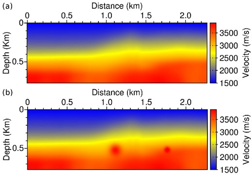
Smooth P-wave model used as background model (a). Smooth P-wave model with two Gaussian perturbations added in depth (b).
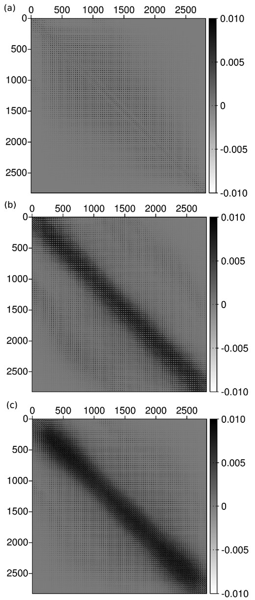
Rescaled operators. Gauss–Newton operator HGN(m0) associated with the standard FWI misfit function (a), product of the Beylkin and the Born modelling operators |$\scr {B}(m_0)J(m_0)$| (b), Gauss–Newton operator |$H_{{\rm GN}}^{g}(m_0)$| (c).
To complement the analysis of these operators, the distribution of their eigenvalues is presented in Fig. 4. The spectrum of the standard Gauss–Newton operator presents a rapid decrease after the 200th eigenvalue. In contrast, the spectrum of the operator |$\scr {B}(m_0)J(m_0)$| and its associated normal operator |$H^{g}_{GN}(m_0)$| presents a slower decrease. This indicates the better conditioning of these operators compared to the standard Gauss–Newton operator.
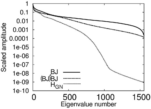
Eigenvalue distribution of the Gauss–Newton operator associated with the standard FWI misfit function HGN(m0), the product of the Beylkin and the Born modelling operators |$\scr {B}(m_0)J(m_0)$|, the Gauss–Newton operator |$H_{{\rm GN}}^{g}(m_0)=\left(\scr {B}(m_0)J(m_0)\right)^{*}\scr {B}(m_0)J(m_0)$| associated with the modified misfit function g(m).
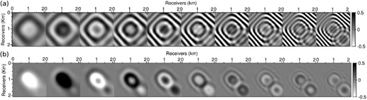
Residuals in the source/receiver plane, for the 10 different frequencies from 3 to 12 Hz. L2 norm-based standard residuals (a). Migrated/Demigrated residuals (b).
In contrast, the imprint of the two inclusions is clearly visible in the residuals associated with the modified misfit function g(m) from lower frequencies. Already at 4 Hz, the effect of the second inclusion is visible in the residuals. Another difference is that the long-offset residuals are filtered. The migration/demigration operation results in an emphasis on the information associated with near-offset data. The illumination angle filtering resulting from the application of the operator |$\scr {B}(m_0)^{*}\scr {B}(m_0)$| to the data residuals can be related to the mathematical definition of the Beylkin operator and its adjoint, given in Appendix B. From the formulas (B17) and (B18), it can be seen that a multiplication by a factor (cos (θ) + 1)2 is applied to each residual components, which implies the observed emphasis of small illumination angles.
The gradients associated with the standard L2 norm-based misfit function and the modified misfit function are presented in Fig. 6. For a fair comparison, the same scaling is applied to both of the gradients. As expected, the L2 norm-based gradient [Fig. 6(a)] mainly focusses on the first inclusion, which is centred with respect to the acquisition system, and is larger in size. In contrast, the gradient of the modified misfit function provides a more balanced update for the large and small inclusions [Fig. 6(b)]. On the other hand, positive/negative oscillations around the inclusions are introduced, which resembles limited bandwidth effects observed in the reconstruction provided by asymptotic linearized inverse methods [see for instance Thierry et al. (1999a)]. The balance in the inclusion reconstruction and these oscillations are the imprint of the introduction of the Beylkin operator in the misfit function.
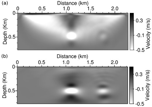
Gradients computed for the two inclusions case study. Standard L2 norm-based gradient (a). Modified misfit function gradient ∇g(m) (b).
4.3 Application to the Marmousi model
The properties of the modified misfit function are analysed on the acoustic Marmousi2 model (Martin et al.2006). The exact and initial models are presented in Fig. 7. The domain size is 3 km deep and 17 km wide. The initial model is obtained by a Gaussian smoothing of the exact model with a correlation length equal to 375 m. This yields an accurate initial model. A fixed-spread surface acquisition system with 336 sources and receivers located at 50 m depth and spread along the upper water layer from x = 0.15 km to x = 16.9 km each 50 m is used. The frequency bandwidth for the data goes from 3 to 7.5 Hz. The P-wave velocity in the water layer is supposed to be known. It is kept constant, equal to 1500 m s−1, throughout the inversion process. The spatial discretization h for the finite-difference scheme is set to 25 m both in vertical and horizontal directions, which yields a 141 × 681 point discrete model. As mentioned preliminary, the operator |$\scr {B}(m_0)$| is discretized over a coarse grid with a discretization step |$\tilde{h}=100$| m. A fine frequency discretization is used, with a sampling of 0.25 Hz, which yields a data set with 19 discrete frequencies from 3 to 7.5 Hz. Numerical experiments presented in the sequel show that this fine discretization is required for the asymptotic pre-conditioning to be accurate.
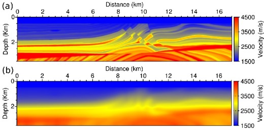
Marmousi 2 P-wave exact (a) and initial (b) models.
The standard L2 norm residuals are compared with the migrated/demigrated residuals for five frequencies (3, 4, 5, 6 and 7 Hz) in Fig. 8. As in the previous experiment, for each frequency, a panel presents the real part of the residuals in the source/receiver plane. The migration/demigration process operates a strong filtering of the residuals associated with long-offset data and focusses on near-offset data. This is again the impact of the angle illumination filtering associated with the Beylkin operator. This may result in emphasizing reflection data at the expense of diving-wave data.
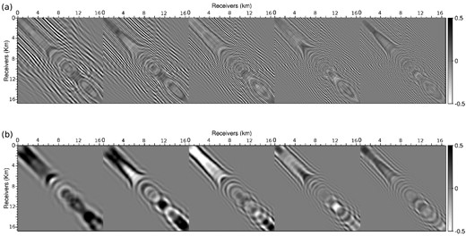
Marmousi2 case study. Normalized residuals for the frequencies 3, 4, 5, 6 and 7 Hz. Standard L2 norm-based residuals (a) and migrated/demigrated residuals (b).
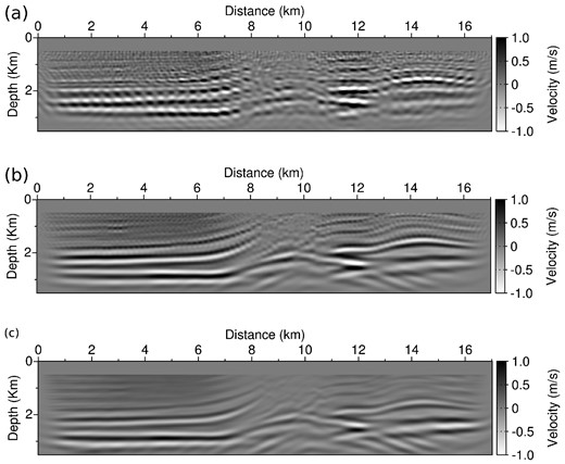
Model update |$\scr {B}(m_0)(d_{{\rm cal}}(m_0)-d_{{\rm obs}})$| which would be provided by the Beylkin method (a), standard FWI gradient in the initial Marmousi 2 model (b) and modified misfit function gradient in the initial Marmousi 2 model ∇g(m0) (c).
The effect of the frequency sampling on the accuracy of the Beylkin operator |$\scr {B}(m_0)$| is presented in Fig. 10. Coarsening the frequency sampling to 0.5 and 1 Hz yields important artefacts on the gradient of the modified misfit function g(m). This effect is consistent with the formulas (42) and (43). The asymptotic convergence of |$\scr {B}(m_0)$| towards a left inverse of J(m0) requires the domain of integration in frequency to go continuously from 0 towards the infinity. Approximating this integral with a too coarse frequency sampling decreases the accuracy of the approximation.
Marmousi2 case study. Effect of the frequency sampling. Gradient of the modified misfit function g(m) with 1, 0.5 and 0.25 Hz samplings.
The effect of the compression used to compute the Beylkin operator |$\scr {B}(m_0)$| is also presented in Fig. 11. Not surprisingly, if the operator is approximated on a too coarse grid in space, spatial aliasing will not be totally removed in the gradient of the modified misfit function g(m). The coarsening which is used should be actually chosen consistently with the expected resolution. Here, as the frequency content of the data does not exceed 7.5 Hz, a spatial discretization of 100 m is enough for obtaining a smooth P-wave velocity gradient.
Marmousi2 case study. Effect of the compression level used for computing the Beylkin operator |$\scr {B}(m_0)$|. Gradient of the modified misfit function g(m) with 400, 200 and 100 m grids.
The inversion results obtained with the modified misfit function after 3 and 10 l-BFGS iterations are presented in Fig. 12. These results have to be compared with those obtained using the standard L2 norm after 3, 10 and 40 l-BFGS iterations, presented in Fig. 13. A diagonal pre-conditioning based on the pseudo-Hessian operator is included in the l-BFGS algorithm for the standard FWI method (Shin et al.2001). Details on practical implementation of this pre-conditioning strategy can be found in Métivier & Brossier (2015).
Marmousi2 case study. Reconstructed models after 3 (a) and 10 (b) l-BFGS iterations using the modified misfit function g(m).
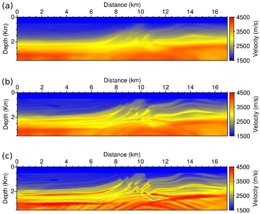
Marmousi2 case study. Reconstructed models after 3 (a), 10 (b) and 40 (c) l-BFGS iterations using standard FWI with a diagonal pre-conditioner.
While in standard FWI the estimation first focusses on the shallow part and progressively reconstructs the deeper parts of the model, the modification introduced by the Beylkin operator allows to reconstruct deep structures in the very first iterations. This is due to the focusing of the method on smaller illumination angles and reflection data. A high-resolution estimation of the subsurface model is yielded directly in the first iterations. The progress between the third and the tenth iterations indicates a reconstruction of amplitudes rather than the building of interfaces. As a counterpart, the shallow part of the model, sampled both by diving and reflected waves, is less constrained when using the modified misfit function. The estimation in this zone is less accurate than the ones obtained with a standard FWI method. This seems a limitation of the approach, caused by the filter applied to diving waves induced by the asymptotic operator.
To further investigate this issue, vertical P-wave velocity profiles are presented in Fig. 14. Theses profiles are taken at x = 5 km, x = 9 km and x = 14 km, respectively. The profiles obtained after 40 iterations of pre-conditioned l-BFGS follow almost exactly the exact profiles, excepted in depth, where the true amplitude of the reflectors is not recovered. The results obtained after 10 l-BFGS iterations using the modified misfit function show that the trend is recovered both in shallow and deep parts around the initial model profile. This suggests that the low-frequency part of the model is not updated. The reflectors are thus located at their proper locations, but a lack of low-wavenumber updates is visible. This analysis is confirmed in Fig. 15 where the frequency content of the vertical profiles is presented. The profiles obtained from 40 iterations of pre-conditioned l-BFGS recover the low-frequency part of the exact profiles. The profiles obtained after 10 iterations of l-BFGS using the modified misfit function clearly present a gap in the low-wavenumber part of the spectrum.
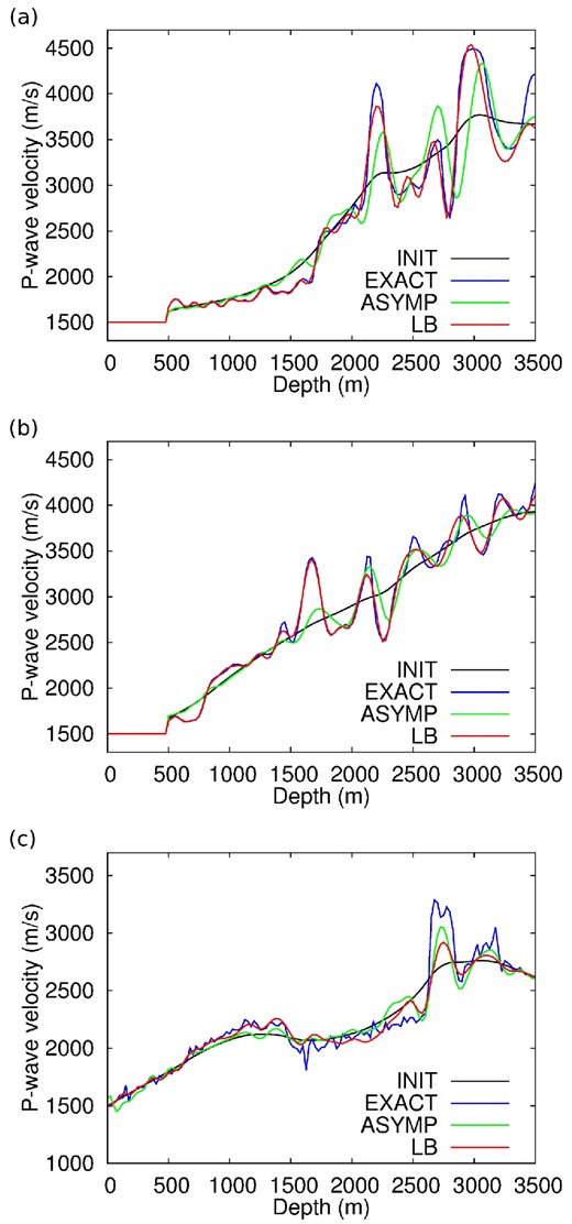
Marmousi2 case study. Vertical logs of P-wave velocity models extracted at x = 5 km (a), x = 9 km (b) and x = 14 km (c). Exact model (red), initial model (black), reconstructed model after 10 iterations of modified FWI (green) and reconstructed model after 40 iterations of standard FWI (blue).
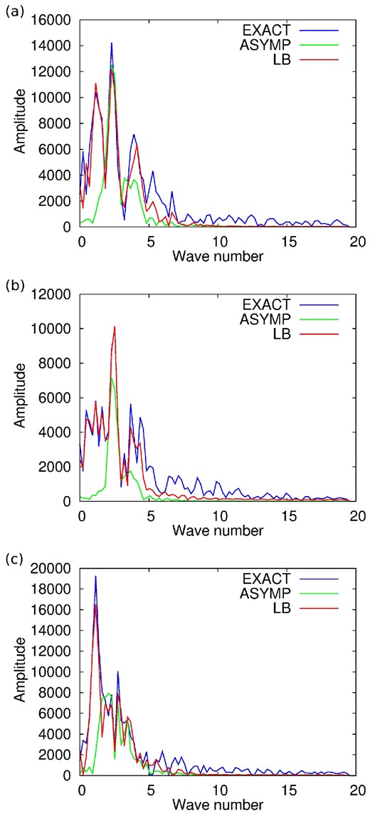
Marmousi2 case study. Wavenumber spectrum of the P-wave velocity update along vertical logs extracted at x = 5 km (a), x = 9 km (b) and x = 14 km (c). Exact update (blue), update obtained after 10 iterations of modified FWI (green) and update obtained after 40 iterations of standard FWI (red).
4.4 Application to the synthetic Valhall model
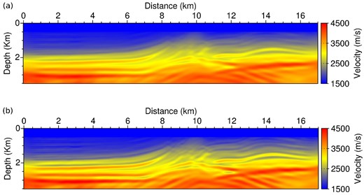
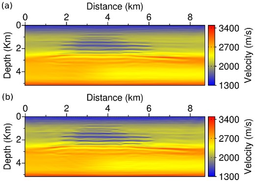
The numerical experiments are completed by an application on the synthetic Valhall model presented in Fig. 16, together with the initial model which is used. The model is deeper than the Marmousi 2 model; its lateral extension is smaller: it is 5 km deep and 8.7 km wide. It presents interesting low-velocity layers associated with the presence of gas and a strong curved reflector located above z = 3 km. As in the Marmousi 2 experiment, a fixed-spread surface acquisition system is used with 173 sources and receivers located at 50 m depth and spread along the horizontal axis from x = 0 km to x = 8.65 km each 50 m. The frequency bandwidth for the data goes from 3 to 7 Hz. The frequency sampling is equal to 0.25 Hz, as in the Marmousi 2 experiment, which yields a data set with 17 discrete frequencies. The spatial discretization h is set to 25 m both in vertical and horizontal directions, which yields a 207 × 349 point discrete model. Compared to the Marmousi2 case study, the reduction of the maximum offset of the acquisition system and the good quality of the initial velocity model emphasize the importance of reflected waves rather than diving waves for recovering the exact P-wave velocity model. It is expected that in this situation, the approach based on the modified misfit function g(m) provides good results.
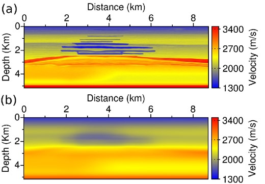
Exact (a) and initial (b) models for the Valhall case study.
In Fig. 17, the residuals associated with the standard L2 norm-based FWI are compared to the residuals after migration and demigration using the Beylkin operator |$\scr {B}(m_0)$| and its adjoint. The same presentation as for the previous case studies is used: the five panels are associated with the frequencies 3, 4, 5, 6 and 7 Hz. Each panel is a presentation of the residuals in the source/receiver plane. The migration/demigration operation focusses again on near-offset data, detrimental to far-offset data.
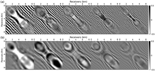
Normalized residuals for the frequencies 3, 4, 5, 6 and 7 Hz. Standard L2 norm-based residuals (a) and migrated/demigrated residuals (b).
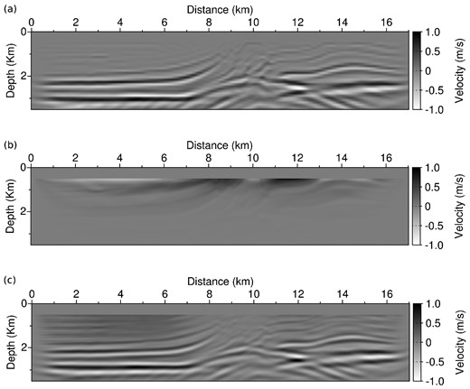
In Fig. 18, the model update δm associated with the Beylkin migration (eq. 66) is compared to the gradient in the initial model associated with the standard FWI misfit function and the modified misfit function. As a migration result, the model update δm [Fig. 18(a)] yields a good reconstruction of the interfaces present in the exact velocity model presented in Fig. 16. Because of the coarse sampling of |$\scr {B}(m_0)$|, the update suffers from spatial aliasing, although this is less visible than in the Marmousi 2 experiment. The FWI gradient [Fig. 18(b)] focusses mainly on the shallow part of the model. A smooth, low-wavenumber update of the zone above the first kilometre is provided, associated with transmitted energy. Two dark wings also appear connecting both lateral extremities of the acquisition to the zone in the centre. These artefacts are due to the incompleteness of the acquisition. The modified misfit gradient [Fig. 18(c)] appears as a smoother version of δm. The spatial aliasing effect is removed. The amplitude of the model update is corrected. A very shallow reflector at z = 0.5 km also appears, which is not visible in δm.
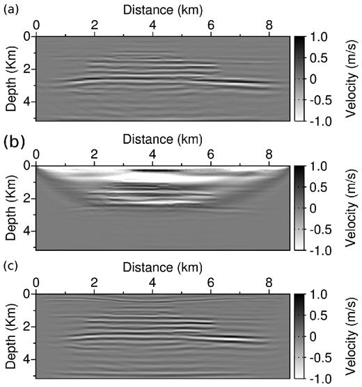
Model update |$\scr {B}(m_0)(d_{{\rm cal}}(m_0)-d_{{\rm obs}})$| which would be provided by the Beylkin method (a), standard FWI gradient in the initial Valhall model (b) and gradient of the modified misfit function g(m) in the initial Valhall model (c).
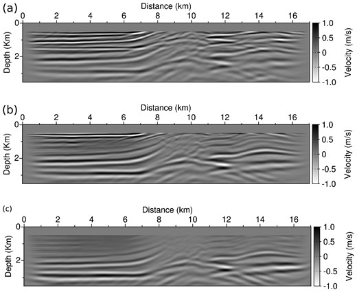
The results obtained after 5 and 10 l-BFGS iterations using the modified misfit function g(m) are presented in Fig. 19. After five iterations, the main interfaces already appear clearly in the estimated model. The gas layers are accurately reconstructed. The main reflector at z = 3 km is well delineated from x = 1 km to x = 7 km. Additional iterations (from 5 to 10) allow to restore more accurately the amplitude and to improve slightly the resolution of the estimation. The results obtained after 5, 10 and 20 l-BFGS iterations using the standard FWI misfit function with a diagonal pre-conditioning strategy are presented in Fig. 20. At least 20 iterations are required for the standard FWI method to be able to reconstruct satisfactorily the gas layers in the middle of the domain [Fig. 20(d)]. However, the deepest part of the model, including the main reflector at z = 3 km, is less precisely estimated in this case. In comparison, this reflector is more accurately estimated when the modified misfit function g(m) is used. Here, the standard FWI method faces an important difficulty as increasing the number of iteration does not seem to improve further the solution. After 40 iterations, the main reflector appears more clearly only between x = 1 km, x = 2 km and x = 5 km, x = 7 km. The reconstruction of the gas layers starts to reveal some instabilities, despite the synthetic data are not corrupted by any noise. Note for instance the high-amplitude artefact appearing in red at z = 2.5 km, x = 5 km [Fig. 20(e)]. This instability is not observed when the modified misfit function g(m) is used.
Reconstructed model after 5 (a) and 10 (b) l-BFGS iterations using the modified misfit function g(m).
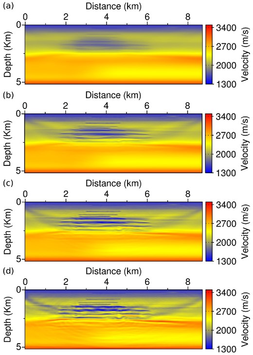
Reconstructed model after 5 (a), 10 (b), 20 (c) and 40 (d) l-BFGS iterations using standard FWI with a diagonal pre-conditioner.
To complement this analysis, P-wave velocity vertical profiles of the reconstructed models are presented in Fig. 21. The profiles are extracted at x = 2.1 km, x = 4.4 km and x = 6.5 km. The reconstructed models obtained after 10 l-BFGS iterations using the modified misfit function g(m) and 20 l-BFGS iterations using standard FWI with a diagonal pre-conditioning are compared to the exact and the initial models. For the three logs, the model reconstructed using the modified misfit function is the closest to the exact profile, especially in depth (z > 2 km). This is consistent with the observations made on the 2-D reconstructions. However, as for the Marmousi2 case study, the updates obtained using the modified misfit function seems to lack low-wavenumber content. This observation is supported by the 1-D spectral analysis of these updates presented in Fig. 22.
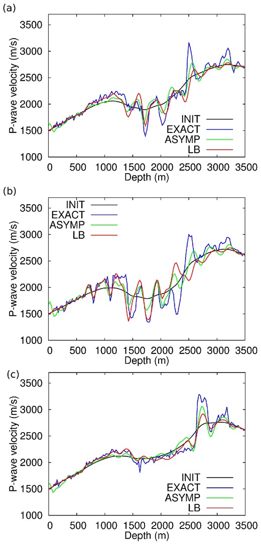
Valhall case study. Vertical logs of P-wave velocity models extracted at x = 2.1 km (a), x = 4.4 km (b) and x = 6.2 km (c). Exact model (blue), initial model (black), reconstructed model after 10 iterations of modified FWI (green) and reconstructed model after 40 iterations of standard FWI (red).
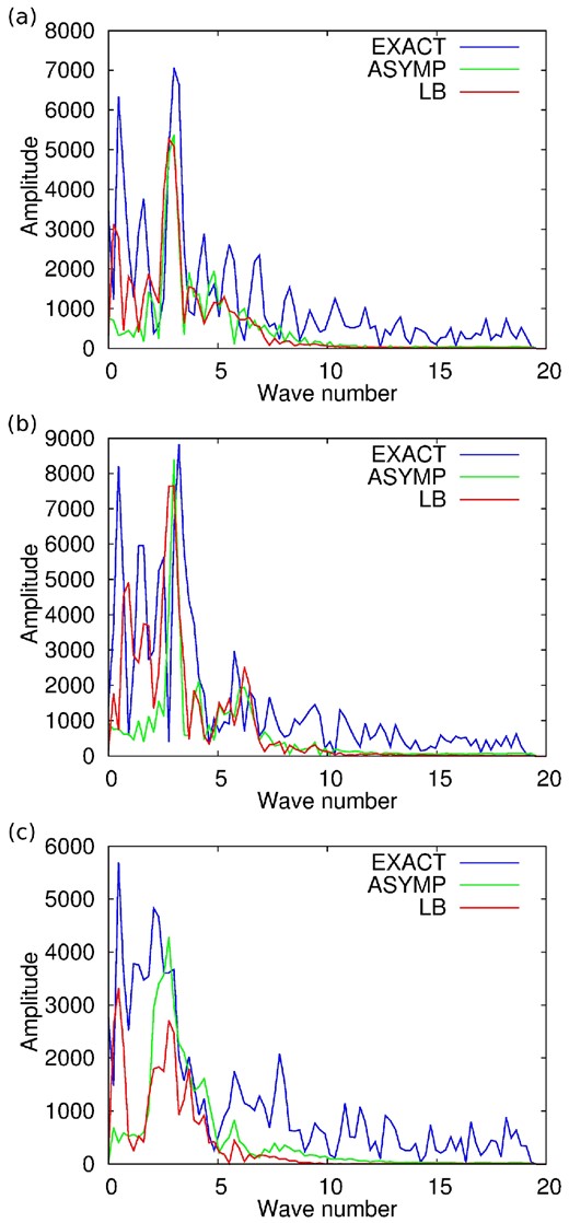
Valhall case study. Wavenumber spectrum of the P-wave velocity update along vertical logs extracted at x = 2.1 km (a), x = 4.4 km (b) and x = 6.2 km (c). Exact model (red), initial model (black), reconstructed model after 10 iterations of modified FWI (green) and reconstructed model after 40 iterations of standard FWI (blue).
5 DISCUSSION
The results presented in this study provide important information. First, it should be noted that despite working with FWI far from the high-frequency regime, with a seismic data bandwidth comprised between 3 and 7.5 Hz, the asymptotic approximation still brings valuable information on the propagation operators involved in the inversion process. In particular, the left inverse devised by Beylkin from the asymptotic approximation of the Born modelling operator is still a relatively good left pre-conditioner for the ‘true’ Born modelling operator, computed with the full wavefield. This is emphasized in the first case study, where these operators are presented (Fig. 3). This result indicates that the asymptotic approximation is meaningful and could be used to build pre-conditioners even far from the high-frequency regime.
Second, introducing the Beylkin operator within the FWI scheme through the definition of the modified misfit function (56) is not without having some consequences on the inversion process. The filtering applied on the data residuals associated with wide scattering angles should be underlined. The method amounts to significantly focus on the short-offset data rather than long-offset data, as can be seen in the migrated/demigrated residuals in Figs 5, 8 and 17. This makes the method similar to a migration process rather than a full waveform inversion process as long-offset data maybe not accounted for accurately.
From the expression of the Beylkin operator, one could think, however, that this effect is counterbalanced by the frequency weighting strategy embedded in this operator. Indeed, from eq. (B17), one can see that a scaling factor equal to the inverse of the frequency is applied to the data, which gives more weight to low-frequency data rather than higher frequency data in the inversion. This makes possible to enhance the reconstruction of low-wavenumber components of the P-wave velocity model, according to the expression (67). This strategy, named as spectral shaping, is presented in Lazaratos et al. (2011) and Plessix (2013). However, the numerical results presented here tend to indicate that the compensation induced by this frequency weighting is not sufficient: the illumination angle based filtering has a stronger influence on the reconstruction process.
Nevertheless, if the low-wavenumber components of the solution is contained in the initial model, it appears that the modification of the misfit function improves significantly the convergence speed of the minimization process. This suggests that the modified misfit function could be used for instance for accelerating non-linear quantitative migration algorithms, such as in Métivier et al. (2011) and Métivier (2011) for the reconstruction of the acoustic impedance around a well with walkaway data, with a given velocity model. In Zhou et al. (2014a,b), a method is proposed for the coupled reconstruction of the low-wavenumber components of the P-wave velocity model and the high-wavenumber components of the P-impedance. At each iteration of the process, a non-linear minimization has to be performed to compute the reflectivity model with the current velocity model: the method proposed here could also be applied to accelerate this process.
In terms of practical implementation, the computation of the Beylkin operator amounts to the computation of a large-scale dense matrix. This requires a significant computational effort and has a strong impact on its memory requirement. A coarsening strategy has to be applied in accordance with the frequency content of the data which is inverted. Practicing an off-line computation of the operator as a prior stage to the inversion reduces the computational cost as the quantities from the Beylkin operator are computed only once. As a counterpart, this requires the ability of storing the dense matrix on the coarse grid. A trade-off could be found by recomputing some of the matrix entries at each iteration. Another possibility also consists in using compression strategies, such as the ACA method to devise H-matrix approximation of the Beylkin operator (Bebendorf 2008).
Finally, the approach is presented here in the frequency domain for the sake of simplicity. However, the strategy can be extended to time-domain inversion. In the work of Beylkin (1985), the derivation of the migration operator was initially performed in the time domain. In practice, the frequency-domain inversion requires a fine sampling of the frequency integration domain (see Fig. 10). The computational gain associated with frequency-domain approach for FWI relies on the possibility of exploiting data redundancy and invert for few discrete frequencies. Therefore, in this case, it seems that there are no advantages to keep a frequency-domain approach. The method could thus be considered for accelerating the convergence of time-domain least-squares migration algorithms, which are known to be intensively time consuming.
6 CONCLUSION
This study presents a strategy for combining concepts inherited from linearized inversion with non-linear least-squares inversion scheme such as FWI. In particular, the preserved-amplitude migration operator derived by Beylkin (1985) from the adjoint of the asymptotic approximation of the Born modelling operator is used to define a modified misfit function. The gradient associated with this new misfit function shares some similarities with the standard L2 norm-based FWI gradient. It is the cross-correlation of the wavefield diffracted by any single localized perturbation of the discrete medium with residuals. The difference with standard FWI is that the residuals on which the method applies are first migrated/demigrated using the Beylkin operator and its adjoint. The Hessian of this modified misfit function is shown to tend asymptotically towards the identity operator. As an inverse problem, the minimization of this misfit function is thus a better posed problem, as the trade-off between parameters is reduced.
It is observed numerically that despite working far from the high-frequency regime, the modified misfit function has indeed a diagonal dominant Hessian operator. However, the modification of the misfit function through the Beylkin operator implies a focussing of the method on small illumination angle data, detrimental to large-offset data. As a consequence, the sensitivity of the misfit function to diving waves is reduced, and the method is efficient only in a migration regime. This indicates that this strategy could be employed for accelerating non-linear quantitative migration algorithms.
The results which have been obtained suggests that the asymptotic approximation should be an appropriate tool to better condition the FWI problem. Future studies will be led to investigate the use of the Beylkin operator for building directly an approximate inverse of the Hessian operator. This pre-conditioner could be used in the framework of a truncated Newton method. This strategy is expected to be efficient especially for the multiparameter case for which trade-offs between different classes of parameters (for instance P-wave velocity and density in the acoustic approximation) make the computation of a decoupled estimation a strongly difficult task.
It is important to emphasize that the asymptotic approximation can be extended to account for anisotropy, attenuation and the propagation of elastic waves. Extension to multi-arrival can also be performed to improve the accuracy and the impact of an asymptotic pre-conditioning. Therefore, the approach which is developed here is not limited to the acoustic case and is hopefully a preliminary step towards the definition of more general pre-conditioners for FWI.
This study was partially funded by the SEISCOPE consortium (http://seiscope2.osug.fr), sponsored by BP, CGG, CHEVRON, EXXON-MOBIL, JGI, PETROBRAS, SAUDI ARAMCO, SCHLUMBERGER, SHELL, SINOPEC, STATOIL, TOTAL and WOODSIDE. This study was granted access to the HPC resources of the Froggy platform of the CIMENT infrastructure (https://ciment.ujf-grenoble.fr), which is supported by the Rhône-Alpes region (GRANT CPER07_13 CIRA), the OSUG@2020 labex (reference ANR10 LABX56) and the Equip@Meso project (reference ANR-10-EQPX-29-01) of the programme Investissements d'Avenir supervised by the Agence Nationale pour la Recherche, and the HPC resources of CINES/IDRIS under the allocation 046091 made by GENCI. The authors thank all the actors of the SEISCOPE consortium research group for their active and constant support, especially Stéphane Operto for helpful and animated discussions.
REFERENCES
APPENDIX A: AMPLITUDE AND TRAVELTIME COMPUTATION FOLLOWING THE RAY THEORY
The following quantities have to be computed for the asymptotic approximation
the traveltime maps T(x; r), T(x; y);
the amplitude maps A(x; r), A(x; y).
Compute the traveltimes from the receiver r using the eikonal solver.
Perform a back ray tracing from the point x to the receiver r using the gradient of the traveltime ∇T(x; r).
Store the components p1 and p2 at x and at the receiver r.
Get the initial condition for the paraxial ray tracing and solve the paraxial equations (A4).
Compute j(x; r) following formula (A8).
APPENDIX B: COMPUTATION OF THE BEYLKIN INTEGRAL OPERATOR |$\scr {B}$| AND ITS ADJOINT |$\scr {B}^{*}$|
The integral operator |$\scr {B}$| is defined through its kernel, which depends on the function h(xr, xs, ω) defined in eq. (38). For the sake of simplicity, the explicit formulation of |$\scr {B}$| is given for the 2D mono-parameter case (constant density is assumed).
