


Summary
We invert for motions at the surface of Earth’s core under spatial and temporal constraints that depart from the mathematical smoothings usually employed to ensure spectral convergence of the flow solutions. Our spatial constraints are derived from geodynamo simulations. The model is advected in time using stochastic differential equations coherent with the occurrence of geomagnetic jerks. Together with a Kalman filter, these spatial and temporal constraints enable the estimation of core flows as a function of length and time-scales. From synthetic experiments, we find it crucial to account for subgrid errors to obtain an unbiased reconstruction. This is achieved through an augmented state approach. We show that a significant contribution from diffusion to the geomagnetic secular variation should be considered even on short periods, because diffusion is dynamically related to the rapidly changing flow below the core surface. Our method, applied to geophysical observations over the period 1950–2015, gives access to reasonable solutions in terms of misfit to the data. We highlight an important signature of diffusion in the Eastern equatorial area, where the eccentric westward gyre reaches low latitudes, in relation with important up/downwellings. Our results also confirm that the dipole decay, observed over the past decades, is primarily driven by advection processes. Our method allows us to provide probability densities for forecasts of the core flow and the secular variation.
1 INTRODUCTION
The past decade has seen the advent of geomagnetic data assimilation techniques, aiming at modeling the core state by considering constraints not only from geophysical observations, but also from our knowledge of the core dynamics (Fournier et al. 2010). This approach, widely developed to study the dynamics of surface envelopes (ocean and atmosphere), is particularly suited if one aims at either predicting or understanding a dynamical systems (this latter activity being usually referred to as reanalysis). In the context of the geodynamo, reanalyses are promising in the perspective of imaging unobserved quantities (such as the magnetic field, the flow or the buoyancy flux deep in the fluid outer core), and thus isolating mechanisms responsible for the generation of the time-varying Earth’s magnetic field. On the other hand, forecasts aim at proposing future probability densities for the evolution of the field that constrains our spatial environment, with implication in space weather – see, for instance, the damages from cosmic rays on low Earth orbiting satellites as they pass through areas of low magnetic intensity such as the South-Atlantic anomaly (Heirtzler 2002; Aubert 2015).
Several avenues have been followed to handle those two questions. One is to use 3-D forward simulations of the geodynamo (Liu et al. 2007; Fournier et al. 2013) to derive the state of the core (magnetic, velocity and codensity fields) using the primitive induction, momentum and heat equations, given observations of the radial magnetic field at the core–mantle boundary (CMB). However, because of the huge numerical cost required to reach Earth-like regimes, those simulations are presently run using unrealistic dimensionless parameters, implying too large dissipation processes – see, for example, the discussions by Cheng & Aurnou (2016) and Bouligand et al. (2016). Dynamo simulations are nevertheless able to provide static and kinematic images of the core consistent with geomagnetic field models (e.g. Christensen et al. 2010). However, their current development prevents from appropriately modeling the dynamics associated with rapid changes of the secular variation (the rate of change of the magnetic field, or SV).
An alternative avenue consists in considering reduced models able to relatively enhance the role played by magnetic forces, as initiated by Canet et al. (2009) or Labbé et al. (2015) under the quasi-geostrophic (QG) assumption. However, such models are not yet operational. In the absence of entirely satisfying prognostic models, SV predictions propagated by core surface motions have been carried out, using piecewise stationary flows (Beggan & Whaler 2009; Whaler & Beggan 2015). These first pragmatic attempts are operational but do not include important information contents, for instance on the temporal correlation of the flow, or the subgrid errors associated with the unresolved CMB magnetic field at small length scales. These issues have been addressed in the framework of stochastic processes (see van Kampen 2007), which appear able to estimate the probability density function (PDF) of time-dependent core surface flows. Gillet et al. (2015b) proposed a reanalysis of QG transient motions over 1940–2010 by means of a weak formalism, while Gillet et al. (2015a) used instead an Ensemble Kalman Filter (EnKF, see Evensen 2003) to predict the magnetic field PDF in the context of the IGRF-12 (International Geomagnetic Reference Field – 12th generation, Thébault et al. 2015). In this latter proof-of-concept study, subgrid errors were accounted for with an augmented state approach (e.g. Reichle et al. 2002). We refer for instance to Miller et al. (1999) for an illustration of the stochastic EnKF efficiency to describe the evolution of the model state PDF, and to Buizza et al. (1999) for the representation of model uncertainties through stochastic processes, and their impact on the prediction scores.
In the present work, we merge for the first time spatial information provided by numerical simulations with temporal constraints brought by specifically chosen stochastic processes. The former is obtained by free runs of a 3-D geodynamo model, as initiated by Fournier et al. (2011), and has been previously used to infer series of independent snapshot core flows from geomagnetic field models by Aubert (2013, 2014). The latter extends the algorithm developed by Gillet et al. (2015a), in particular by considering a contribution from core surface magnetic diffusion that improves the analysis of Aubert (2014). Furthermore, here we follow and complement an idea supported by Amit & Christensen (2008), and derive diffusion from cross-covariances involving up/downwellings and the gradient of the magnetic field below the CMB.
The present work displays similarities with the work of Baerenzung et al. (2014, 2016), as it aims to depart from mathematical smoothing often employed to ensure spectral convergence (the large-scale hypothesis, see Holme 2015), possibly enhancing the footprint of unresolved small length-scale structures in the SV at large length scales. Through this work, we present the first validation, with synthetic experiments, of the ability to recover time-dependent core flow features. It is also the first attempt at multiepoch assimilation that uses spatial information from geodynamo while analysing recent geomagnetic data.
We present in details our algorithm in Section 2. In Section 3.1, we test and validate our approach with synthetic experiments, in order to quantify our ability to infer information on observable and unobservable quantities of the core state. Next in Section 3.2, we apply our algorithm in a geophysical configuration with a reanalysis of the COV-OBS.x1 model (Gillet et al. 2013, 2015a) over 1950–2015. We finally discuss in Section 4 possible applications, such as hypothesis testing or the forecast of the geomagnetic field PDF.
2 MODELS AND METHODS
2.1 Spatial cross-covariances from geodynamo simulations
Summary of the notations used throughout this study. The state x shall here be considered as a generic notation (either b or u or e).
| Physical space | Spectral space | Meaning | Truncation degree |
|---|---|---|---|
| Br | B | Radial magnetic field | |$1-n_b^{{\rm CE}}$| |
| |$\overline{B}_{r}$| | b | Large-scale radial magnetic field | 1 − no |
| |$\tilde{B}_{r}$| | |$\tilde{\bf b}$| | Small-scale radial magnetic field | |$n_{o}+1-n_b^{{\rm CE}}$| |
| u | u | Surface core flow | 1 − nu |
| er | e | Subgrid errors | 1 − no |
| d | d | Diffusion | 1 − no |
| eo | Main field observation errors | 1 − no | |
| bo | Main field observations | 1 − no | |
| |$\dot{\bf e}^o$| | SV observation errors | |$1-\dot{n}_{o}$| | |
| |$\dot{\bf b}^o$| | SV observations | |$1-\dot{n}_{o}$| | |
| |$\hat{\bf x}(t)$| | Background state | ||
| 〈x〉 | Time-average state | ||
| x*(t) | Reference state | ||
| x†(f) | State time Fourier transform | ||
| xf(t) | Forecast | ||
| xa(t) | Analysis | ||
| x΄(t) | Analysis error xa − x* | ||
| |$n_b^{{\rm CE}}$| | Truncation degree of CE magnetic field | 30 | |
| nu | Truncation degree of core flow | 18 | |
| no | Truncation degree of observed magnetic field | 14 | |
| |$\dot{n}_{o}$| | Truncation degree of observed SV | 14 |
To build the spatial prior of our model, we use a forward integration of a geodynamo simulation, the Coupled Earth (CE) model (Aubert et al. 2013). It solves the momentum, codensity and induction equations under the Boussinesq approximation, for an electrically conducting fluid within a spherical shell (of aspect ratio 0.35 between the inner core and the CMB), assuming no-slip (respectively free-slip) conditions at the inner (respectively outer) boundary. It furthermore accounts for a heterogeneous mass-anomaly flux at both the inner and outer boundaries, together with a gravitational coupling between the inner core and the mantle. Its construction leads to similarities with the Earth’s dynamo from both a static (magnetic field morphology) and a kinematic (secular variation and core flow structure) point of view.
We use NCE = 1505 realizations from the CE dynamo to infer statistics on the magnetic field and the flow, truncated at respectively |$n_u^{{\rm CE}}=18$| and |$n_b^{{\rm CE}}=30$|. All realizations are snapshots of a free run, separated by 90 yr—dimensionless times are scaled into years as in Aubert (2015), following Lhuillier et al. (2011). The dimensionless magnetic field is scaled into physical units by matching its spatial spectrum at the CMB to that of the COV-OBS field model, averaged over 1840–2010.
2.2 A time-dependent stochastic model
Furthermore, because of the geometric attenuation from the CMB upward to the Earth’s surface, and the larger power contained into the lithospheric field at short wavelengths, the main field is resolved only for degrees n ≤ no = 14. Only the large-scale fraction of the radial magnetic field |$\overline{B}_{r}$| is available in eq. (10) to retrieve information on u. The unresolved component |$\tilde{B}_{r}={B}_{r}-\overline{B}_{r}$| nevertheless generates observable SV: the subgrid electromotive force (e.m.f.) associated with the unresolved field is a major source of uncertainty in eq. (10), and the principal limitation in the estimation of core motions from geomagnetic data (Eymin & Hulot 2005; Pais & Jault 2008). Properly accounting for these subgrid errors is crucial to obtain an unbiased estimate of the core state and its associated posterior errors (Gillet et al. 2015b; Baerenzung et al. 2016).
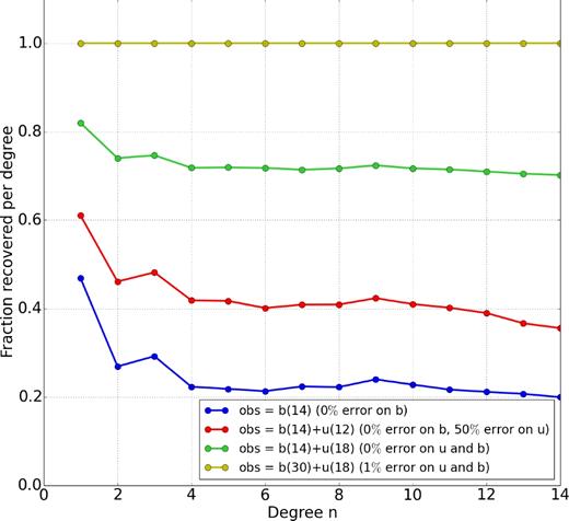
Relative fraction of energy recovered on diffusion as a function of harmonic degree, when estimating diffusion using eq. (18), where b and u are snapshots from the CE dynamo, in several configurations: Br and |${\boldsymbol u}_H$| are almost entirely known up to degrees, respectively, 30 and 18 (yellow); Br and |${\boldsymbol u}_H$| are entirely known up to degrees, respectively, 14 and 18 (green); Br is entirely known up to degree 14 and the half of |${\boldsymbol u}_H$| (in energy) is known up to degree 12 (red); Br only is entirely known up to degree 14 (blue), with no information on |${\boldsymbol u}_H$|.
2.3 Diffusion from the CE dynamo
Fig. 1 shows how much of the true CE diffusion can be retrieved depending on the information considered in the inverse problem (18). Each curve is obtained from the ratio between the Lowes spectrum of the analysis error (difference between the analysis (18) and the CE dynamo diffusion) and the spectrum of the CE dynamo diffusion (spectra are averaged over the NCE snapshots of the CE dynamo). Ignoring cross-covariances involving the flow, the observable field at degrees below 14 allows us to recover only 20 per cent of the diffusion from degree 4 onwards (and about 55 per cent for the lowermost degrees). In a case where the flow would be entirely known up to degree 18, errors would drop to less than 30 per cent at high degrees, and to less than 20 per cent for the dipole. An intermediate error of about 40–60 per cent is found if 50 per cent of the flow is known up to degree 12—a reasonable error estimate following Gillet et al. (2015b). In the unrealistic case where both the field and the flow are almost entirely known up to degrees, respectively, 30 and 18, 100 per cent of the CE diffusion is retrieved from the linear estimate (18). This shows that, assuming that cross-covariances provided by the dynamo are meaningful, it is possible to retrieve information on the time changes of surface diffusion from knowledge of only the surface magnetic field and flow.
These results have important consequences on the analysis of the SV, and encourage us to analyse diffusion in our algorithm (see Section 2.4). Indeed, through eq. (18) diffusion is now allowed to be responsible for rapid SV changes, because it is linearly related to the flow. This reflects the modulation by up/downwellings of magnetic field gradients below the CMB. Contrary to 3-D models that would explicitly calculate diffusion, our 2-D model for the advection/diffusion of Br at the CMB relies on an inversion: in the forward integration of eq. (11), the diffusion term |$d({\boldsymbol u}_H,e_r)$| is obtained from eq. (18) with |${\sf R}_ {bb}={\sf 0}$| and |${\sf R}_ {uu}={\sf 0}$|. We consider that our misestimation of the true diffusion in this case is negligible (cf. Fig. 1), in particular in comparison with subgrid errors (and see fig. 9 in Aubert 2013).
2.4 Augmented state Kalman filter
Now that the forward system is set-up, we describe the algorithm used to invert for the core state. We seek the most likely trajectory x(t) given observations of the main field and its secular variation, statistics on their associated errors and statistics on the core state described in the above sections. We write bo and |$\dot{\bf b}^o$| the vectors containing observations of the main field and SV Gauss coefficients (described up to degrees no and |$\dot{n}_{o}$|), eo and |$\dot{\bf e}^o$| their associated (unbiased) errors, the statistics of which are described by the covariance matrices |${\sf R}_{bb}={\mathbb {E}}\left[{\bf e}^o{\bf e}^o{}^T\right]$| and |${\sf R}_{\dot{b}\dot{b}}={\mathbb {E}}\left[\dot{\bf e}^o\dot{\bf e}^o{}^T\right]$|, respectively.
In contrast with the canonical EnKF (Evensen 2003), we do not update, for each analysis step, the forecast covariance matrices |${\sf P}_{zz}^f=E[({\bf z}^f-\hat{\bf z}^f)({\bf z}^f-\hat{\bf z}^f)^T]$| and |${\sf P}_{bb}^f=E[({\bf b}^f-\hat{\bf b}^f)({\bf b}^f-\hat{\bf b}^f)^T]$| with the empirical estimate built from the ensemble of realizations. Constructing such empirical matrices with well-constrained cross-covariances would indeed require an ensemble of size Nm at least 10 times larger than the size of the matrix to be inverted in eq. (20) (see Fournier et al. 2013), that is, in our case several thousands. Even if possible (though demanding) to achieve computationally, it is not meaningful to provide such a sophisticated algorithm if we consider that our model does not account for any deterministic dynamics for the flow (see Section 4.3). Furthermore, any future algorithm including a deterministic physics will most probably be costly, and only operational with ensemble sizes of a few hundreds at most, as it is the case in the community studying surface fluid envelopes (e.g. Clayton et al. 2013). To by-pass this difficulty, numerical approximations are employed, as inflation to avoid ensemble collapse (see Hamill et al. 2001), or localization to produce well-conditioned matrices (e.g. Oke et al. 2007). However, this latter is difficult to operate when working in the spectral domain.
for a vanishing analysis error (a model state very well constrained by the data), the forecast covariance matrices become |${\sf P}_{uu}^f=\alpha _u{\sf P}_{uu}$| and |${\sf P}_{ee}^f=\alpha _e{\sf P}_{ee}$|;
on the opposite, if the innovation vector |${\bf y}^{ko}(t_a)-{\sf H}^k{\bf z}^{kf}(t_a)$| vanishes in eq. (20), the forecast covariance matrix shall represent the whole model statistics, which (this is our working hypothesis) are defined by the CE dynamo covariances, that is, |${\sf P}_{uu}^f={\sf P}_{uu}$| and |${\sf P}_{ee}^f={\sf P}_{ee}$|.
In both cases cross-covariances between u and e are ignored when building |${\sf P}_{zz}$|. The latter choice (ii) may appear suboptimal to recover time changes in the core state, given the temporal correlation of core motions and analyses errors (see appendix A in Gillet et al. 2015b), while the former choice (i) might lead to underestimate the dispersion within the ensemble of flow solutions. These issues are discussed further in Sections 3.1 and 4.1. Concerning the analysis of b, the Kalman gain matrix |${\sf K}_{bb}$|, in eq. (19), is almost identity, due to the very small observation error variances entering |${\sf R}_{bb}$| (see Gillet et al. 2015a, fig. 4). Thus, the choice for |${\sf P}_{bb}^f$| does not really affect the results: inversions performed with the whole CE dynamo statistics (|${\sf P}_{bb}^f={\sf P}_{bb}$|) and with its scaled version (|${\sf P}_{bb}^f={\Delta t^a}^2{\sf P}_{\dot{b}\dot{b}}$|) actually show negligible differences.
The impact of errors on the analysis for diffusion should in principle be considered when building |${\sf R}_{yy}$| for eq. (20). Here again, we will consider two configurations. In the first one, |${\sf P}_{dd}^a$| is simply ignored. In a second one, it is estimated once for all from the statistics of an ensemble of diffusion analysis errors obtained from the CE snapshot realizations using eq. (18). We shall see that these two cases lead to very similar ensemble average solutions, with very close posterior diagnostics (as defined in Section 2.5).
The present work improves the proof-of-concept study by Gillet et al. (2015a), where diffusion processes were ignored. Our scheme makes possible for diffusion errors to alter the forecast, and uncertainties on diffusion analyses will transpire into a larger spread within the ensemble of flow realizations. Furthermore, we derive covariances on |${\boldsymbol u}_H$| and er from the CE dynamo, whereas Gillet et al. were using a QG topological constraint for the flow, ignoring other spatial cross-covariances in both |${\sf P}_{ee}$| and |${\sf P}_{uu}$| to prevent ill-conditioning.
Our approach also differs from the single-epoch algorithm of Aubert (2013, 2014), since the core state is here time-stepped with a (stochastic) dynamical model, carrying information from one epoch to the other. Our treatment of er also differs from that of Aubert (see Section 2.1): we consider that an analysis of |$\tilde{\bf b}$| cannot be used to estimate er in eq. (11)—the reason why it is modeled here through the stochastic equation (14). Indeed, from twin experiments with the CE dynamo, we found that only a small fraction (about 20 per cent) of the true unresolved field |$\tilde{{\bf b}}$| can be recovered from the knowledge of the large-scale field b and of the cross-covariances between them (not shown). Note that, in order to tackle this issue, Aubert (2015) improved his series of algorithms by generating each analysis within his ensemble of snapshot solutions starting from a random realization sampling the whole CE covariances (and not from the CE average as in Aubert 2014). The main steps for the forecast and analysis are summarized in Table 2.
Summary of the augmented state Kalman Filter as implemented in this study (with an ensemble of size Nm = 50). The core state is defined as x = [bT uT eT]T. We refer to the main text for the definition of matrices.
| 1. Forecast |
| |${{\mathrm{d}}{\bf u}/{\mathrm{d}}t+\tau _{u}^{-1}\left({\bf u}-\hat{\bf u}\right)={\boldsymbol \zeta }_u(t),}$| |
| |${{\mathrm{d}}{\bf e}/{\mathrm{d}}t+\tau _{e}^{-1}{\bf e}={\boldsymbol \zeta }_e(t),}$| |
| ${{\bf d}({\bf b},{\bf u})=\hat{\bf d} + \left[\begin{array}{ll}\displaystyle {\sf P}_{db} \quad\displaystyle {\sf P}_{du} \end{array}\right] \left[\begin{array}{rl}\displaystyle {\sf P}_{bb} \quad\displaystyle {\sf P}_{bu}\\
\displaystyle {\sf P}_{ub} \quad\displaystyle {\sf P}_{uu} \end{array} \right]^{-1} \left[\begin{array}{l}
\bf b-\hat{\bf b}\\
{\bf u}-\hat{\bf u} \end{array}\right],}$ |
| |${{\mathrm{d}}{\bf b}/{\mathrm{d}}t = {\sf A}({\bf b}){\bf u} + {\bf e} + {\bf d}({\bf b},{\bf u}),}$| |
| 2. Analysis |
| |${{\bf b}^{a}(t_a)= {\bf b}^{f}(t_a) + {\sf P}_{bb} \left[{\sf P}_{bb} + {\sf R}_{bb}\right]^{-1} \left({\bf b}^o(t_a)-{\bf b}^{f}(t_a)\right),}$| |
| zf(ta) = [uf(ta)T ef(ta)T]T , with ${{\sf P}_{zz} = \left[\begin{array}{ll}\displaystyle \alpha _u{\sf P}_{uu}\quad \displaystyle {\sf 0}\\
\displaystyle {\sf 0} \qquad\quad\displaystyle \alpha _e{\sf P}_{ee} \end{array}\right],}$ |
| |${{\bf d}^{0} = \hat{\bf d} + {\sf P}_{db}{\sf P}_{bb}^{-1}[{\bf b}^{a}-\hat{\bf b}],}$| |
| |${{\bf y}^{o}=\dot{\bf b}^o-{\bf d}^{0},}$| |
| for i ∈ [1 : 5] |
| |${{\bf z}^{a}(t_a)= {\bf z}^{f}(t_a) + {\sf P}_{zz}{\sf H}^T \left[{\sf H}{\sf P}_{zz}{\sf H}^T + {\sf R}_{yy}\right]^{-1} \left({\bf y}^{o}(t_a)-{\sf H}{\bf z}^{f}(t_a) \right),}$| |
| ${{\bf d}^{a}=\hat{\bf d} + \left[\begin{array}{ll}\displaystyle {\sf P}_{db} \quad \displaystyle {\sf P}_{du} \end{array}\right] \left[ \left[\begin{array}{ll}\displaystyle {\sf P}_{bb}\quad \displaystyle {\sf P}_{bu}\\
\displaystyle {\sf P}_{ub}\quad \displaystyle {\sf P}_{uu} \end{array}\right] + \left[\begin{array}{cc}\displaystyle {\sf R}_{bb} \quad\displaystyle {\sf 0}\\
\displaystyle {\sf 0} \qquad\displaystyle {\sf R}_{uu} \end{array}\right] \right]^{-1} \left[\begin{array}{l}\bf b^{a}-\hat{\bf b}\\
{\bf u}^{a}-\hat{\bf u} \end{array}\right],}$ |
| |${{\bf y}^{o}=\dot{\bf b}^o-{\bf d}^{a},}$| |
| end |
2.5 Posterior diagnostics
3 RESULTS
3.1 Synthetic experiments
3.1.1 Construction of the reference trajectory
We initialize the reference trajectory from one realization of the CE dynamo, before the stochastic model defined by eqs (12) and (27) is time-stepped from epoch ts = 1950 to te = 2020. Before to go further, we emphasize that our forward model has been constructed such that a non-negligible part of the SV is associated with diffusion (about 10 per cent of the total SV in power, for all length scales, see Fig. 2). Temporal variations of diffusion correlate with those of the flow. As a consequence, the contribution from diffusion is not restricted to low frequencies. At first sight, this may appear surprising since diffusion derives from the slowly varying main field. However, radial diffusion at the CMB is enslaved to the magnetic field at and below the core surface, which is dynamically coupled to core motions. The link between diffusion and a core flow stretching and twisting magnetic field lines below the CMB transpires in the analysis illustrated with Fig. 1. As a consequence, diffusion is potentially responsible for rapid SV changes at the CMB, as shown with the reference trajectories of SV Gauss coefficients of different orders in Fig. 2. We have yet to demonstrate that temporal variations of the diffusion are linked to rapid flow variations in a fully self-consistent dynamical model run at parameters closer to Earth’s core values. However, for the mechanistic reasons stated here, we anticipate that this may be the case in the Earth’s core, and we have thus constructed our direct model accordingly.
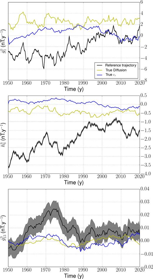
Time-series of SV coefficients (black, ±σ the SV observation error in grey-shaded area) for the reference trajectory, superimposed with the contributions from diffusion (yellow) and subgrid errors (blue). From top to bottom: |$g_1^0, h_6^6$| and |$g_{13}^9$|.
3.1.2 Reanalysis performances: comparative tests
We consider below five configurations, with properties summarized in Table 3. We investigate the impact of accounting for subgrid errors and diffusion in the core state, in the case where we do not scale the model cross-covariances (cases A, B and C). We further analyse the improvement brought by considering scaled model cross-covariances (case D), with both diffusion and er entering the model state. These four cases A–D are run while ignoring |${\sf P}_{dd}^a$| when building |${\sf R}_{yy}$|. A last case E is investigated, where we account for |${\sf P}_{dd}^a$| as described in Section 2.4 (and otherwise similar to the configuration D). It will be discussed at the end of this section.
Posterior diagnostics of eq. (24) for the analysed models xa(t) in the four cases investigated in the synthetic reanalysis. The last column corresponds to the flow misfit, but considering the velocity field only up to degree n = 8.
| Case | d | er | Scaled |${\sf P}$| | |${\sf P}_{dd}^a$| | |$\chi ^2_d$| | |$\chi ^2_e$| | |$\chi ^2_{u}$| | |$\chi ^2_{u{[n\le 8]}}$| |
|---|---|---|---|---|---|---|---|---|
| A | Yes | Yes | No | No | 0.59 | 1.59 | 0.55 | 0.31 |
| B | Yes | No | No | No | 1.76 | |$\diagup$| | 1.51 | 0.70 |
| C | No | Yes | No | No | |$\diagup$| | 1.73 | 0.62 | 0.33 |
| D | Yes | Yes | Yes | No | 0.59 | 1.75 | 0.54 | 0.30 |
| E | Yes | Yes | Yes | Yes | 0.59 | 1.68 | 0.53 | 0.30 |
We first focus on the impact of subgrid errors. If no significant differences on the average SV prediction and the SV forecast dispersion is observed between cases A and B, ignoring er in the model state generates a significant bias between the analysed diffusion and the diffusion of the reference trajectory. This is illustrated with Fig. 3 (top left and bottom left), where we show time-series for the several SV contributions to |$\dot{h}_1^1$|—a coefficient representative of the typical behaviour observed in synthetic series, and the dynamics of which is rich enough to make clear the distinction between SV sources. Indeed, the analysed SV contribution from diffusion in case B shows, for coefficients of all degrees, important offsets at some epochs (e.g. from 1980 onwards on |$\dot{h}_1^1$| series). On the contrary, we manage to recover a significant amount of the reference diffusion when including er in the core state, with a dispersion that most of the time encompasses the reference diffusion. We thus conclude that accounting for er is mandatory to obtain an unbiased estimate of the a posteriori diffusion PDF. In cases A and D, where both er and diffusion are analysed, we obtain a similar performance on the diffusion estimation (see Table 3).
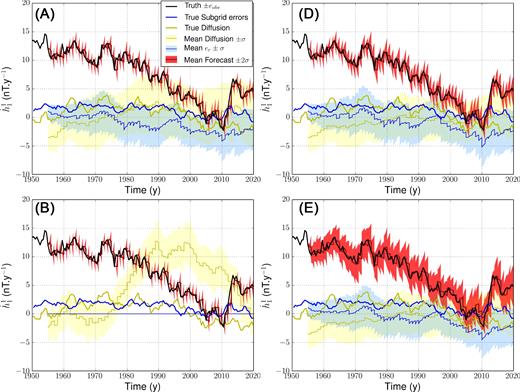
Series of SV coefficients |$\dot{h}_{1}^{1}$| for synthetic experiments: comparison of our model predictions from Nm = 50 reanalyses (average in dark red, ±2σ in light red) with the synthetic observations (reference trajectory in black, ±σ observation errors in grey). Contributions from er (average analysis in blue, ±σ in light blue) and from diffusion (average analysis in yellow, ±σ in light yellow) are also shown, with the reference diffusion in thick yellow and the reference subgrid errors in thick blue. The four cases A (top left), B (bottom left), D (top right) and E (bottom right) are shown.
Fig. 4 presents in case D, the power spectra of the several contributions to the SV. It confirms that the power stored into the analysed diffusion is about 10 per cent that of the observed SV at all length scales. The magnitude of the subgrid errors, similar to that of diffusion at low degrees, appears slightly larger towards small length scales (n ≥ 9). In Fig. 5 (upper and middle rows), we show examples of flow coefficients time-series, accounting or not for er. Ignoring subgrid errors, we find a significant bias between the reference and analysed flows for all but the largest length-scale coefficients: the reference flow trajectory lays outside the a posteriori distribution provided by the ensemble spread. Accounting for er, this inconsistency is canceled. The bottom row of Fig. 5 shows example of flow estimates in case D: if the spread within the ensemble of analyses has been reduced, the ensemble of solutions nevertheless encompasses the reference trajectory at all periods, showing that scaling covariance matrices has helped to better target the reference trajectory. The good fit to SV changes with a biased analysis in case B arises at the expense of a strong aliasing: the analysed core flow shows too large a power spectrum from spherical harmonic degree n ≥ 4, as illustrated in Fig. 6. This drawback disappears as er is reinstated in the model state (case A). By scaling matrices (case D), we obtain a flow solution presenting an even lower average spectrum, without increasing the analysis error (i.e. a simpler solution as close to the reference trajectory).
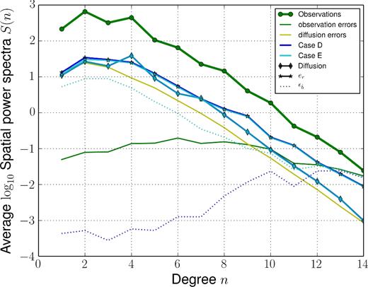
Time-average SV spatial power spectra: spectrum |$\displaystyle \left\langle {\mathscr R}_*\right\rangle (n)$| for the reference SV trajectory (green circled thick line), for observation errors (thin green line), and for our estimate of the errors on diffusion (thin yellow) obtained from the diagonal elements of |${\sf P}_{dd}^a$|. We show in blue (cases D) and cyan (case E), the spectra, at the analysis step, for the contributions from diffusion |$\displaystyle \left\langle {\mathscr D}\right\rangle (n)$| (diamonds), from subgrid errors |$\displaystyle \left\langle {\mathscr E}\right\rangle (n)$| (stars), and for the dispersion within the ensemble of SV predictions (dotted lines).
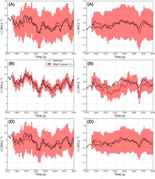
Core flow coefficients series from synthetic experiments for |$t_{1}^{0c}$| (left) and |$t_{8}^{1c}$| (right): comparison of Nm = 50 reanalyses (ensemble mean in dark red, ±2σ in light red) with the reference trajectory (black), in cases A (top), B (middle) and D (bottom).
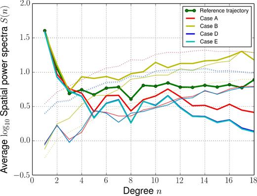
Core flow time-average power spectra |$\displaystyle \left\langle {\mathscr S}\right\rangle (n)$| in cases A (red), B (yellow), D (blue) and E (cyan), for the ensemble average |$\hat{\bf u}$| (thick lines), the analysis error |${\boldsymbol \delta }_u$| (thin lines) and the dispersion within the ensemble |${\boldsymbol \epsilon }_u$| (dotted lines). The green circled line shows |$\displaystyle \left\langle {\mathscr S}\right\rangle (n)$| for the reference trajectory u*. Blue and cyan spectra almost superimpose.
As mentioned in Section 2.4, one may wonder whether using scaled matrices would not lead to underestimate a posteriori uncertainties. This is actually not the case, as illustrated in Fig. 6 where, for cases A and D, the spectrum for the spread within the ensemble of flow solutions is larger than the spectrum for the bias between u* and |$\hat{\bf u}$|. The same spectra in case B clearly lead to discard this configuration. The dispersion seems slightly less overestimated in case D than in case A. This observation is confirmed with the diagnostics ξu, e, d of eq. (25), shown in Fig. 7 as a function of time, for cases A, B and D: in case A (respectively D), we overestimate by a factor about 1.8 (respectively 1.4) the uncertainties on the flow and on diffusion (i.e. the posterior dispersion is a bit conservative), while it is strongly underestimated in case B. We also overestimate the uncertainties on subgrid errors (by a factor about 2) in both cases A and D. Note a warm-up period of about 5–10 yr before the algorithm reaches approximately steady misfit values. If both cases D and A show similar scores in Table 3 for the flow and diffusion, the diagnostics ξu, d tend to favour case D.
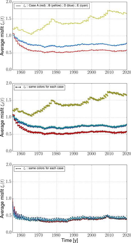
Time evolution of the misfits ξu (top), ξd (middle) and ξe (bottom), given in eq. (25), in cases A (red), B (yellow), D (blue) and E (cyan).
We observe also in the spatial domain the bias observed in the spectral domain, as illustrated with the snapshot surface flow maps in Fig. 8: cases A and D (including er) are much closer to the reference trajectory than case B (no er). The strong aliasing in case B is obvious on the map of the horizontal divergence. To a lesser extent, case A also shows a larger amount of meanders than the simplest case D. The strong bias obtained for the average model as er is ignored is confirmed by normalized misfit values larger than unity for both diffusion and core motions (see Table 3). On the contrary, the three cases A, C and D accounting for er show far less biases for both observed and unobserved quantities: the relative error on core motions for degrees n ≤ 8 decreases to about 30 per cent. However, since the power in core flows is larger towards long periods, the misfits and spectra discussed so far are dominated by the time-average state, and give little information about the time changes of the core state.
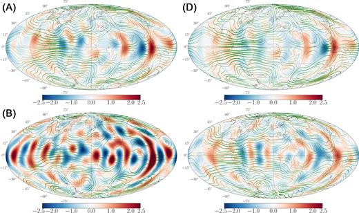
Maps of the horizontal divergence of the flow (red–blue colour scale, in century−1) and of the flow (green stream function) at the CMB, for the average analysis in 2015, in cases A (top left), B (bottom left), D (top right) and for the reference trajectory (bottom right). The thicker the stream function, the stronger the velocity norm (rms velocity over the CMB: 13.28 km yr−1).
We now investigate more closely the core flow resolution as a function of wave number and period, and present in Fig. 9, for the four cases, the ratio |${\mathscr C}(n,f)$| defined by eq. (26). The comparison proposed in Fig. 9 (top left and bottom left) clearly stresses that ignoring er (case B), almost no information on flow fluctuations is retrieved from degree n ≥ 3, while a decent amount of information is obtained up to degree n ≃ 10 for the lowermost frequencies in case A. We also visualize with Fig. 9 (top right) that ignoring diffusion but accounting for er (case C) generates a much less severe mismatch than ignoring er but including diffusion (the worst case B). This confirms that a significant part of the flow may be retrieved under the frozen flux approximation even when this assumption is not exact (and see the snapshot core flow inversions from dynamo simulations by Rau et al. 2000). Still, since improving our knowledge of the flow indirectly improves our estimate of diffusion, we obtain a slightly better reanalysis in case A than in case C: we conclude that if it is mandatory to include er in the core state, it is also worth accounting for diffusion in our algorithm.
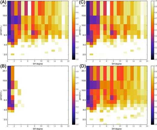
Resolution function |${\mathscr C}$| as a function of spherical harmonic degree and period, in cases A (top left), B (bottom left), C (top right) and D (bottom right). Black (respectively white) corresponds to 0 per cent (respectively 100 per cent) difference between the reference and analysed trajectories.
We now specifically focus on case D with both er and diffusion, but scaling the model covariance matrices according to the stochastic prior dispersion (see Section 2.4). While the scaling eq. (21) only marginally improves diagnostics dominated by long periods (see Fig. 6 and Table 3), Fig. 9 (bottom right) shows that it allows us to slightly better recover rapidly changing flow patterns, especially towards small length scales. We witness here that allowing at each analysis step for a too large innovation (the prior constraint on the model increment in cases A–C is weaker than in case D), we lose some constraints on the transient motions. For those reasons, even if no significant improvement is seen for slow core flow changes, we are inclined to favour case D (which also provides simpler solutions and misfits ξu, d closer to one). We compare in Fig. 10, for our preferred case D, the spatial distribution of the contribution from diffusion to the SV at the CMB. We overall find the correct amplitude (of the order of ±5 nT yr−1), and are able to localize some of the main diffusion patches, as for instance in the Eastern hemisphere between ±40° latitude. The largest patterns appear in the equatorial area. These are found to correlate well with the main up/downwellings at the CMB (compare the maps of diffusion and |$\nabla _h\cdot ({\boldsymbol u}_H)$| in Fig. 8).
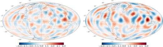
Map of diffusion (nT yr−1) at the CMB from our analysed state in 2015: reference state (right) and ensemble average analysis in case D (left).
We finally compare case D to the last configuration E, where in addition errors on the analysis of diffusion are accounted for. Surprisingly, we see very little changes concerning both the scores of Table 3, the diagnostics in Fig. 7, resolution charts |${\mathscr C}(n,f)$| (not shown) or the flow spectra (Fig. 6). The latter almost superimpose in the two cases not only for the ensemble average flow, but also for the flow dispersion and the average analysis error. Interestingly, the ensemble average diffusion and subgrid errors (as well as their associated dispersion) are also very similar in the two cases (see Fig. 3). The main difference concerns the SV prediction: if these are in average similar in the two cases, a much larger dispersion is found in case E than in case D (see Fig. 3). This behaviour derives from the much looser constraint imposed in case E on the fit to SV data (through |${\sf R}_{yy}$|), and is characterized by enhanced model prediction errors in case E (see Fig. 4).
3.2 Geophysical application
We now apply our algorithm to an ensemble of realizations of the geomagnetic field model COV-OBS.x1, from ts = 1950 to te = 2020. The model prior is the same as that used for the synthetic experiment, that is, the configuration of case D (unless specified otherwise) with τu = 30 yr and Δta = 1 yr. As in the synthetic experiments, analysed flow and diffusion are very similar in cases E and D except for SV predictions, and we only show results for the latter configuration. Performing inversions with instead τu = 100 yr, that is, with a pre-factor αu of 0.020 instead of 0.067 in eq. (21), only minor changes are observed on the ensemble average solution.
3.2.1 Contributions to the secular variation
During the whole studied time-span, the dispersion within the ensemble of SV forecasts is large enough to include the observed SV changes within ±2σ, even when jerks occur during the most accurate satellite era (see Fig. 11). Our algorithm thus provides a coherent estimate of the PDF for the SV coefficients in this geophysical context. Subgrid errors and diffusion both represent about 20 per cent of the total dipole decay, and potentially contain a non-zero average contribution. The same observations holds for a non-dipole SV coefficient such as |$\dot{h}_2^1$|, shown in Fig. 11 (right). Note that COV-OBS.x1 from 2015 onwards is the result of a prediction, built on magnetic records prior to 2014.6 and on the time cross-covariances of the magnetic model prior (Gillet et al. 2015a). For those reasons, observations errors in our study drastically increase after 2015, leading to the widening of the ±2σ values in Fig. 11.
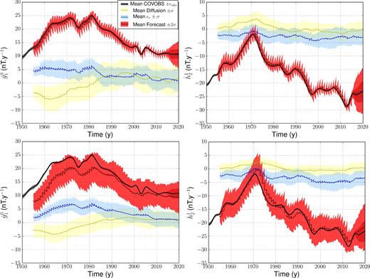
Series of SV coefficients |$\dot{g}_{1}^{0}$| (left) and |$\dot{h}_{2}^{1}$| (right): for the COV-OBS.x1 model (average in black, ±σ in grey), and Nm forecasts from our assimilation algorithm (average in dark red, ±2σ in red), in the configurations D (top) and E (bottom). In blue (respectively yellow) are shown the estimated contributions from er (respectively from diffusion).
As in the synthetic experiments, the spread in SV predictions is larger in case E (Fig. 11, bottom) than in case D. We note a shift towards zero of the average axial dipole decay, larger as |$\dot{g}_1^0$| reaches large values prior to 1985. Still the dispersion in case E encompasses the observed SV, except during the warm-up phase. It is worth noticing that diffusion and subgrid errors show rather similar average trajectories in the two cases E and D, with comparable dispersion.
Our ensemble of forecasts tends, in average, to drive the system towards low SV values. This observation is particularly clear as the recorded SV reaches large values, generating the sawtooth pattern on |$\dot{g}_{1}^{0}$| prior to 1980, and during phases where |$| \dot{h}_2^1|$| increases (see Fig. 11). It is to be expected with the kind of stochastic model we employ, where the most likely flow forecast decays exponentially towards the background flow |$\hat{\boldsymbol u}_H$| in a time τu, driving the average SV forecast naturally to lower values. As such, our average model is not designed to present a predictive power. We associate the better predictions for the dipole decay during the satellite era to the lower value of |$\dot{g}_{1}^{0}$| at that epoch, and to an observed SV decreasing in a similar manner to the AR-1 model.
Our re-analysis confirms that the dipole decay is primarily driven by advection, as suggested in Finlay et al. (2016a). Nonetheless, we find a non-zero negative contribution from diffusion to the dipole decay before 1980 (down to −6 nT yr−1 in the early 1960s). This observation contrasts with the previous estimate by Finlay et al., who found a diffusion contribution almost stationary at about +5 nT yr−1. The difference reflects the impact of flow motions on the analysis of diffusion (see Section 2.3). For the most recent and best documented epochs since 2000, where |$\dot{g}_1^0$| reaches lower values (from 10 to 15 nT yr−1), we still find that diffusion is not the major source of the dipole decay.
3.2.2 Magnetic diffusion and westward gyre
In the spatial domain (see the middle column of Fig. 12), our analysis of diffusion shows localized patches reaching up to ±12 nT yr−1, as for instance below Indonesia. Again, these are in relation with up/downwellings (Fig. 12, right-hand column) that primarily shows up in the equatorial area. This link is not systematic though, because diffusion is not enslaved only to the flow: it also depends locally on the magnetic field morphology. Indeed, the large upwelling to the northeast of Brazil in 1960 is associated with little diffusion. The link between up/downwellings and surface diffusion was suggested by Amit & Christensen (2008), through the poloidal flow component carried by columnar structures. However, we do not retrieve the prominent diffusion feature that they highlight below the Pacific. Here, we associate the localized diffusion patterns in the equatorial belt with the eccentric westward gyre put forward by Pais & Jault (2008). As Aubert (2013) and Gillet et al. (2015b) before us (under respectively a dynamo norm and a QG constraint), we retrieved here this planetary-scale structure in our reanalysis (right-hand column of Fig. 12). We find up/downwelling and the largest signatures of diffusion where the gyre reaches the equatorial area. Although influenced by the primarily equatorial symmetric CE dynamo prior, our solution displays in this area a velocity field that crosses the equator, violating locally the QG assumption, in agreement with the conclusions of Baerenzung et al. (2016).
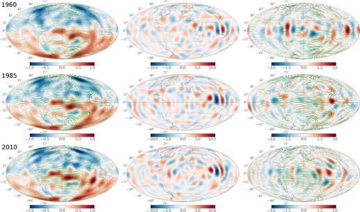
Ensemble average reanalyses at epochs 1960, 1985 and 2010 (from top to bottom) at the CMB from COV-OBS.x1. Left: maps of the main radial field Br (red–blue colour scale, in μT) and of the flow (green stream functions). Middle: maps of the contribution from diffusion to the SV (in nT yr−1). Right: maps of the horizontal divergence of the flow (red–blue colour scale, in century−1) and of the flow (green stream functions).
Interestingly, our estimate of diffusion also differs from that of Chulliat & Olsen (2010). From the analysis of satellite field models, they found below the South Atlantic ocean violations of topological constraints derived from the assumption of an infinitely conducting outer core (namely changes of the magnetic flux passing through areas delimited by null-flux curves, see for instance Jackson 1996), which they interpret as the signature of diffusion. Our solutions do not show particularly large diffusion in conjunction with the South Atlantic Anomaly (see Fig. 12, left-hand and middle columns). We associate the difference with the findings of Chulliat & Olsen to the role played by subgrid processes: they blur our image of null-flux curves, which soften the topological constraints (cf. Gillet et al. 2009). Alternatively, we see a possible correlation between the localized equatorial patches of diffusion and the rapid changes in the secular acceleration (∂2Br/∂t2, see Chulliat & Maus 2014; Chulliat et al. 2015), through flow perturbations around the westward gyre (Finlay et al. 2016b). Indeed strong secular acceleration patterns are found under Indonesia and Central to South America, the location where we also isolate the strongest diffusion and up/downwelling features.
Fig. 12 shows that the westward gyre is present since 1960, suggesting a temporal stability of the largest flow features (the rms velocity over the CMB in 1960, 1985 and 2010 are, respectively, 13.9, 14.0 and 12.3 km yr−1). However, towards the most recent epochs, it strengthens below South America and the Atlantic ocean, at the same time the large upwelling present below NE Brazil around 1960 vanishes. We also note the occurrence of secondary circulations with decadal time-scales, such as the vortices below 30° latitude in the Eastern Pacific hemisphere and those centred around ±30° latitude in the western Pacific, which are present in 1985 but have almost disappeared in 2010. The westward gyre also appears as a complex structure, with modulation of its meanders throughout the studied era. Even though our ensemble average solution does not capture the fastest changes in the core trajectory at small length scales (cf. Fig. 9), maps shown in Fig. 12 suggest nevertheless that some time-dependent meso-scale eddies seem to be robust (see Gillet et al. 2015b; Amit & Pais 2013).
3.2.3 Length-of-day predictions
We now confront the result of our reanalysis to an independent geophysical observation, namely changes in the length of day (LOD). LOD data are here computed from annual means of angular momentum series provided by the International Earth Rotation and Reference System Service (IERS) (the C04 series, see Bizouard & Gambis 2009) cleaned for solid tides (the IERS 2000 model) and for atmospheric predictions from the National Center for Environmental Prediction/National Center for Atmospheric Research (NCEP/NCAR) reanalysis (see Zhou et al. 2006, and references therein). A 1.4 ms cy−1 trend has been removed, corresponding to the observed LOD trend over the past centuries (Stephenson et al. 1984). LOD predictions from our ensemble of flow models are computed using eq. (101) of Jault & Finlay (2015), which accounts for the effect of compressibility on the radial density profile—though very little difference is found with the original formula by Jault et al. (1988).
Fig. 13 shows that during the whole studied time-span, our model provides a convincing prediction for the decadal LOD changes. The recorded geodetic series is captured within the ±σ predictions, and the 1994 local extremum in the LOD is partially caught by the ensemble average reanalysis—we have knowledge of no flow model capable of entirely predicting this bump, an issue first put forward by Wardinski (2005). Focusing during the satellite era, we also note a mismatch between LOD data and our ensemble average prediction, which does not catch the maximum around 2008, contrary to the QG reconstruction by Gillet et al. (2015b)—although the 2008 peak still lays within our ±σ envelope.
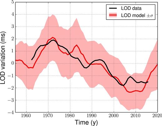
Length-of-day (LOD) variations predicted from our ensemble of reanalyses (average in red, ±σ in red-shaded area), compared with the geodesic data (black). Note that we only plot here the LOD of the reanalysis (and not of forecasts).
3.2.4 Dispersion of the secular variation over 5 yr intervals
Finally, we address the spread of our predicted SV to geophysical observations in a configuration where analyses are performed every Δta = 5 yr. We consider below three configurations: that of case D (CE cross-covariances, τu = 30 yr), a case F where the CE cross-covariances are multiplied by 4 (τu = 30 yr) and a case G similar to case D but with τu = 100 yr instead. Note that the estimates for diffusion, subgrid errors and the flow at the analysis step are not significantly different in those three cases, meaning the analysed model is relatively robust.
SV reanalyses of COV-OBS.x1 data in cases D, F and G are shown in Fig. 14. In case D, the observed SV is almost always embedded within ±2σ of the 5 yr SV forecasts for all coefficients but the axial dipole (see Fig. 14, top). Our model indeed misses the trend towards large |$\dot{g}_1^0$| values recorded prior to 1980—in line with the natural behaviour of average SV forecast mentioned in Section 3.2.1. This observation suggests three possibilities: (i) the cross-covariances, we use from the CE dynamo do not allow enough freedom, (ii) the decay towards the background is too fast (τu too small), or (iii) higher order statistics are needed to mimic the behaviour of the dipole decay in particular, as observed in palaeomagnetic records (Love & Constable 2003) and in numerical simulations (e.g. Bouligand et al. 2005; Fournier et al. 2011).
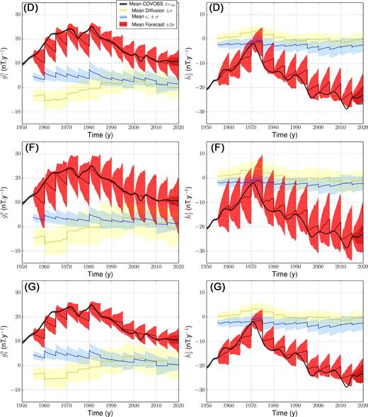
Series of SV coefficients |$\dot{g}_{1}^{0}$| (left) and |$\dot{h}_{2}^{1}$| (right) for an analysis window Δta = 5 yr in case D (top), F (middle) and G (bottom). See the text for details. The legend is the same as in Fig. 11.
We test the first two possibilities with cases, respectively, F and G. The alternative (iii) could be attended using more complex stochastic models (e.g. Buffett et al. 2013). By increasing the model covariances (Fig. 14, middle), the dispersion within the ensemble of SV predictions is enlarged for all coefficients, and a factor of two on the prior model dispersion is enough for the observed dipole decay to lay within ±2σ. By increasing τu (Fig. 14, bottom), the decay of the SV forecast becomes naturally slower, although the dispersion is also reduced, so that case G, as case D, does not always catch the observed |$\dot{g}_1^0$| within ±2σ.
4 SUMMARY AND DISCUSSION
4.1 New insights from our approach
Following earlier strategies developed for geomagnetic data assimilation (Aubert 2015; Gillet et al. 2015a; Whaler & Beggan 2015), the algorithm we present in this study proposes to mix spatial information from Earth-like geodynamo simulations and a temporal information compatible with the frequency spectrum of geomagnetic series, to reanalyse geomagnetic field models within a stochastic, augmented state Kalman filter. We have shown from time-dependent synthetic experiments that subgrid errors that arise from interactions between the unresolved magnetic field at small length scales and core motions must be accounted for. Indeed, ignoring them leads to strong bias and aliasing in the analysed core state. By representing sugbrid errors by means of a stochastic equation, we significantly improve our recovery of the time-dependent core state. Our augmented state algorithm furthermore circumvents the bias encountered for SV predictions by Gillet et al. (2015b), who had implemented the stochastic constraints within a weak formalism (i.e. through covariance matrices instead of time-stepped stochastic equations).
We also propose a new avenue to estimate diffusion at the CMB, from cross-correlations (inferred from geodynamo simulations) between diffusion and both magnetic and velocity surface fields. Indeed, diffusion is related to the magnetic field at and below the core surface, and thus is coupled to core motions. We show from synthetic experiments that a non-negligible amount of diffusion can be recovered. Our analysis furthermore suggests that diffusion must carry a high-frequency content, through its link with up/downwellings. Its amplitude is locally as large as about 10 nT yr−1. Our analysis shows rather different estimations of diffusion in comparison with previous studies: as mentioned in Section 3.2, we find no crucial signature of diffusion associated with the South Atlantic anomaly, but instead a significant contribution on the equator below Indonesia.
4.2 Future evolution of the algorithm
The tool we derived remains nevertheless imperfect, which calls for future methodological developments. Our algorithm indeed does not integrate all the power of the EnKF, essentially in link with our crude estimate of the analysis error cross-covariances (see Section 2.4). Our attempts at approximating these more closely (e.g. using |${\sf P}_{zz}^f= \alpha {\sf P}_{zz} + \left[{\sf I}-{\sf K}_{zz}{\sf H}\right]{\sf P}_{zz}$|, not shown) actually underperform the simpler representations with frozen matrices. This calls for alternatives to localize cross-covariances in the spectral domain (Wieczorek & Simons 2005) if one wishes to avoid computing thousands of realizations.
We have investigated the impact of errors on the analysed diffusion, which should in principle be considered, with a crude estimate of their cross-covariances. We found that adding their contribution to the observation error—through the matrix |${\sf R}_{yy}$| in eq. (20)—only marginally modifies the solutions for the flow and diffusion (average and dispersion), while allowing for a larger SV spread at the analysis steps. This difference is most probably accommodated by the flexible representation of time-correlated model errors through an augmented state—which possibly ingest other sources of uncertainties that are not explicitly accounted for. Accordingly, the impact on the spread in 5 yr (or longer) SV forecasts may appear negligible in comparison with uncertainties associated with our choice of prior information (see Section 3.2.4).
4.3 An hypothesis testing tool
However, the estimate of the surface core trajectory (flow and diffusion) will depend on the considered geodynamo model. In particular, the sensitivity of the analysed diffusion to the chosen dynamo prior calls for further investigations using dynamo simulations run at more extreme parameters (e.g. Aubert et al. 2017; Schaeffer et al. 2017). Our algorithm is by construction flexible: any spatial cross-covariances may be considered. Indeed, one only needs well-conditioned statistics on Br, |${\boldsymbol u}_H$|, er and η∇2Br from any forward model to test different hypotheses, such as the amount of quasi-geostrophy, the need for an asymmetric thermal forcing, etc.
Note also that our algorithm allows for possible changes in the forward (time-integrated) stochastic model. Alternatives to our simple AR-1 representation may be considered, for both subgrid errors and core motions (cf. Section 3.2.4). Furthermore, our AR-1 model may be used as a zero state for comparisons with algorithms using deterministic equations. One could for instance measure if assimilation tools based on prognostic geodynamo models (e.g. Fournier et al. 2013) perform better than the same dynamo spatial statistics embedded in our stochastic algorithm, in either a reanalysis or a forecast framework.
4.4 Towards an operational assimilation tool
In the perspective of developing operational geomagnetic data assimilation tools, our algorithm may be seen as a first step before ingesting direct magnetic records (from satellites, observatories, etc.), instead of their interpolation through Gauss coefficients as in this study. This may require not only the migration of observations at each analysis epochs (as done with virtual observatories, see Mandea & Olsen 2006), but also the coestimation of external sources together with core motions, which calls for further developments. Despite the limitations of its predictive power, we can envision with the strategy developed throughout this study to build IGRF candidate models (in particular the SV for the coming 5 yr together with its associated uncertainties, see Thébault et al. 2015) constrained by core motions.
Acknowledgments
NG and OB were partially supported by the French Centre National d’Etudes Spatiales (CNES) for the study of Earth’s core dynamics in the context of the Swarm mission of ESA. ISTerre is part of Labex OSUG@2020 (ANR10 LABX56), which with the CNES also finance the PhD grant of OB. Numerical computations were performed at the Froggy platform of the CIMENT infrastructure (https://ciment.ujf-grenoble.fr) supported by the Rhône-Alpes region (GRANT CPER07 13 CIRA), the OSUG@2020 Labex (reference ANR10 LABX56) and the Equip@Meso project (referenceANR-10-EQPX-29-01). This is an IPGP contribution.
