


Abstract
Seismic studies indicate that the Earth's inner core has a complex structure and exhibits a strong elastic anisotropy with a cylindrical symmetry. Among the various models which have been proposed to explain this anisotropy, one class of models considers the effect of the Lorentz force associated with the magnetic field diffused within the inner core. In this paper, we extend previous studies and use analytical calculations and numerical simulations to predict the geometry and strength of the flow induced by the poloidal component of the Lorentz force in a neutrally or stably stratified growing inner core, exploring also the effect of different types of boundary conditions at the inner core boundary (ICB). Unlike previous studies, we show that the boundary condition that is most likely to produce a significant deformation and seismic anisotropy is impermeable, with negligible radial flow through the boundary. Exact analytical solutions are found in the case of a negligible effect of buoyancy forces in the inner core (neutral stratification), while numerical simulations are used to investigate the case of stable stratification. In this situation, the flow induced by the Lorentz force is found to be localized in a shear layer below the ICB, whose thickness depends on the strength of the stratification, but not on the magnetic field strength. We obtain scaling laws for the thickness of this layer, as well as for the flow velocity and strain rate in this shear layer as a function of the control parameters, which include the magnitude of the magnetic field, the strength of the density stratification, the viscosity of the inner core and the growth rate of the inner core. We find that the resulting strain rate is probably too small to produce significant texturing unless the inner core viscosity is smaller than about 1012 Pa s.
1 INTRODUCTION
The existence of structures within the inner core was first discovered by Poupinet et al. (1983), who discussed the possibility of lateral heterogeneity from the observation of P-waves traveltime anomalies. These were then attributed to the existence of seismic anisotropy (Morelli et al.1986; Woodhouse et al.1986), with P-waves travelling faster in the north–south direction than in the equatorial plane. Since then, more complexities have been discovered in the inner core: a slight tilt in the fast axis of the anisotropy, radial variations of the anisotropy with a nearly isotropic upper layer, hemispherical variations of the thickness of the upper isotropic layer, an innermost inner core with different properties in anisotropy or attenuation and anisotropic attenuation (See Souriau et al.2003; Tkalčić & Kennett 2008; Deguen 2012; Deuss 2014, for reviews, and references therein).
The seismic anisotropy can be explained either by liquid inclusions elongated in some specific direction (shape preferred orientation, SPO; Singh et al.2000) or by the alignment of the iron crystals forming the inner core (lattice preferred orientation, LPO). In the case of LPO, the orientation is acquired either during crystallization (e.g. Karato 1993; Bergman 1997; Brito et al.2002) or by texturing during deformation of the inner core. Several mechanisms have been proposed to provide the deformation needed for texturing: solid state convection (Jeanloz & Wenk 1988; Weber & Machetel 1992; Buffett 2009; Deguen & Cardin 2011; Cottaar & Buffett 2012; Deguen et al.2013), or deformation induced by external forcing, due to viscous adjustment following preferential growth at the equator (Yoshida et al.1996, 1999; Deguen & Cardin 2009), or Lorentz force (Karato 1999; Buffett & Bloxham 2000; Buffett & Wenk 2001).
Thermal convection in the inner core is possible if its cooling rate, related to its growth rate, or radiogenic heating rate is large enough to maintain a temperature gradient steeper than the isentropic gradient. In other words, the heat loss of the inner core must be larger than what would be conducted down the isentrope. However, the thermal conductivity of the core has been recently reevaluated to values larger than 90 W m−1 K−1 at the core mantle boundary (CMB) and in excess of 150 W m−1 K−1 in the inner core (de Koker et al.2012; Pozzo et al.2012; Gomi et al.2013; Pozzo et al.2014), and this makes thermal convection in the inner core unlikely (Yukutake 1998; Deguen & Cardin 2011; Deguen et al.2013; Labrosse 2014). Inner core translation, that has been proposed to explain the hemispherical dichotomy of the inner core (Monnereau et al.2010), results from a convection instability (Alboussière et al.2010; Deguen et al.2013; Mizzon & Monnereau 2013) and is therefore also difficult to sustain.
Compositional convection is possible if the partition coefficient of light elements at the inner core boundary (ICB) decreases with time (Deguen & Cardin 2011; Gubbins et al.2013) or if some sort of compositional stratification develops in the outer core (Alboussière et al.2010; Buffett 2000; Gubbins & Davies 2013; Deguen et al.2013) so that the concentration of the liquid that crystallizes decreases with time. However, the combination of both thermal and compositional buoyancy does not favour convection in the inner core (Labrosse 2014).
The strong thermal stability of the inner core resulting from its high-thermal conductivity (Labrosse 2014) is a barrier to any vertical motion and other forcing mechanisms need to work against it. This situation has already been considered in the case of deformation induced by preferential growth in the equatorial belt (Deguen & Cardin 2009), and has been shown to produce a layered structure. Deguen et al. (2011) and Lincot et al. (2014) evaluated the predictions of anisotropy from this model and found that although it can induce significant deformation, it is difficult to explain the strength and geometry of the anisotropy observed in the inner core.
In this paper, we consider another major external forcing that was proposed, Maxwell stress. This was first proposed by Karato (1999) who considered the action of the Lorentz force assuming the inner core to be neutrally buoyant throughout. This situation is rather unlikely and, as discussed above, we expect the inner core to be stably stratified. Buffett & Bloxham (2000) have shown that in this case the flow is confined in a thin layer at the top of the inner core, similar to the case discussed above for a flow driven by preferential growth at the equator. However, the growth of the inner core gradually buries the deformed iron and this scenario may still produce a texture in the whole inner core. All these previous studies considered a fixed inner core size and infinitely fast phase change at the ICB. The moving boundary brings an additional advection term in the heat balance which can influence the dynamics. In the context of inner core convection Alboussière et al. (2010) and Deguen et al. (2013) have proposed a boundary condition at the ICB that allows for a continuous variation from perfectly permeable boundary conditions, that was considered in previous studies, to impermeable boundary conditions when the timescale for phase change is large compared to that for viscous adjustment of the topography.
In this paper, we investigate the dynamics of a growing inner core subject to electromagnetic forcing, and include the effects of a stable stratification, of the growth of the inner core and different types of boundary conditions. We propose a systematic study of the dynamics induced by a poloidal Lorentz force in the inner core and develop scaling laws to estimate the strain rate of the flow.
In Section 2, we develop a set of equations taking into account the Lorentz force and a buoyancy force from either thermal or compositional origin. Analytical and numerical results are presented in Section 3, scaling laws for the maximum velocity and strain rate are developed in Sections 4 and 5 and compared to numerical solutions. In Section 6, we use our results to predict the instantaneous strain rates and cumulative strain in the Earth's inner core due to the Lorentz force.
2 GOVERNING EQUATIONS
2.1 Effect of an imposed external magnetic field
The magnetic field produced by dynamo action in the liquid outer core extends up to the surface of the Earth, but also to the centre-most part of the core. Considering for example a flow velocity of the order of the growth rate of the inner core gives a magnetic Reynolds number (comparing advection and diffusion of the magnetic field) of the inner core of about 10−5. This shows that the magnetic field in the inner core is only maintained by diffusion from its boundary.
Two dynamical effects need to be taken into account: the Lorentz force and Joule heating. The Lorentz force acts directly on the momentum conservation, while Joule heating is part of the energy budget and modifies the temperature distribution, inducing a flow through buoyancy forces.
In this paper, we will discuss the effect of the Lorentz force in the case of a purely toroidal axisymmetric magnetic field with a simple mathematical form. The effect of Joule heating in the case of a nongrowing inner core was studied by Takehiro (2010) and will not be investigated further here.
The poloidal magnetic field intensity at the CMB can be inferred from surface observations of the field at the Earth's surface, but both poloidal and toroidal components are poorly known deeper in the core. The root mean square (rms) strength of the field at the ICB has been estimated using numerical simulations to be around a few milliteslas (e.g. Glatzmaier & Roberts 1996; Christensen & Aubert 2006). It can be also constrained by physical observations: for example, Koot & Dumberry (2013) give an upper bound of 9–16 mT for the rms field at the ICB by looking at the dissipation in the electromagnetic coupling, while Gillet et al. (2010) suggest 2–3 mT from the observation of fast toroidal oscillations in the core. Buffett (2010) obtains similar values from measurements of tidal dissipation. Numerical simulations also predict a strong azimuthal component Bϕ at the vicinity of the inner core, possibly one order of magnitude higher than the vertical component Bz (Glatzmaier & Roberts 1996), though this depends on the magnitude of inner core differential rotation.
Buffett & Wenk (2001) have considered the effect of the azimuthal component of the Lorentz force resulting from the combination of the Bz and Bϕ components of the magnetic field. We will focus here on the effect of the azimuthal component of the magnetic field, for which the associated Lorentz force is poloidal and axisymmetric. The flow calculated by Buffett & Wenk (2001) is decoupled from the flow induced by the azimuthal component of the magnetic field, and thus the total axisymmetric flow can be obtained by simply summing the two flows.
One of the most intriguing feature of the Earth's magnetic field is the existence of reversals. However, since the Lorentz force depends quadratically on the magnetic field, its direction is not modified by a reversal of the field. For simplicity, we will consider that the magnetic field is constant in time.
The magnetic field inside the inner core is calculated by diffusing the field from the ICB. The magnetic Reynolds number for the inner core being very small, B is not advected by the flow. Because the seismic observation of anisotropy is of large scale, and also because low-order toroidal component penetrates deeper inside the inner core, only the lowest order of the azimuthal component of the magnetic field is taken into account, following the work of Karato (1999) and Buffett & Bloxham (2000).
The potential part of the Lorentz force can only promote a new equilibrium state but no persisting flow. We are thus only interested in the non potential part of the Lorentz force, shown in Fig. 1. Eq. (3) provides a characteristic scale for the force as |$B_0^2/\mu _0 r_{ic}$|.
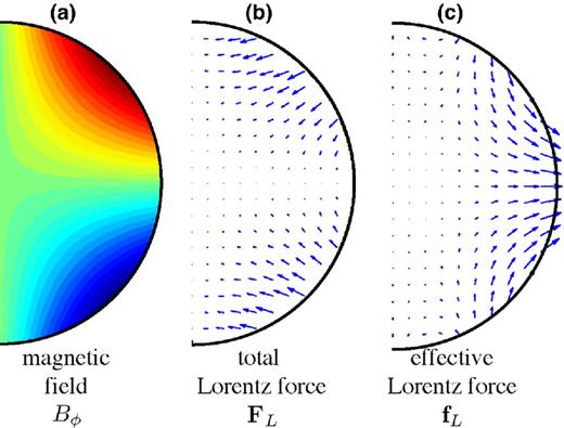
Meridional cross sections showing the intensity of the magnetic field (a), the Lorentz force FL (b) and the nonpotential part of the Lorentz force f L as defined in eq. (3) (c).
Karato (1999) investigated the effect of the Maxwell stress by applying a given normal stress on the ICB. This is different from our study, where, as in Buffett & Bloxham (2000), we consider a volumetric forcing, as shown on Fig. 1, and not a forcing on the surface of the inner core.
2.2 Conservation equations
2.2.1 Conservation of mass, momentum and energy
We consider an incompressible fluid in a spherical domain, with a newtonian rheology of uniform viscosity η, neglecting inertia. Volume forces considered here are the buoyancy forces, with density variations due to temperature or compositional variations, and the Lorentz force as defined above.
The density depends on both the temperature T and the light element concentration c. We define a potential temperature as Θ = T − Ts(r, t), with Ts(r, t) the isentropic temperature profile anchored to the liquidus at the ICB, and introduce a potential composition |$C=c-c^s_{ic}(t)$|, where |$c^s_{ic}(t)$| is the composition of the solid at the ICB. We will consider separately the effects of composition and temperature, but both can induce a density stratification, which is quantified through a variation of density Δρ which is either ραTΘ or ραCC, where ρ is the reference density, and αT and αC the coefficients of thermal and compositional expansion, respectively. Because the potential temperature and composition are solutions of mathematically similar equations, we will use a quantity χ which is either the potential temperature Θ or composition C. In this paper, quantities that apply for both cases will have no subscript, whereas we will use T for quantities referring to the thermal stratification, and C for compositional stratification.
As discussed in Deguen & Cardin (2011), the inner core is stably stratified when the source term S(t) is negative, and no convective instability can develop. In this paper, we will focus on this case, with either ST(t) or SC(t) negative.
2.2.2 Growth of the inner core
2.3 Dimensionless equations and parameters
2.3.1 Definition of the dimensionless quantities
ξ(t) and Pe(t) characterize the growth of the inner core. The Péclet number Pe(t) compares the apparent advection from the moving boundary to diffusion. A large Péclet number thus corresponds to a fast inner core growth compared to the diffusion rate. In the case of a nongrowing inner core, Pe = 0, |$\dot{S}(t)=0$| and the relevant timescale is no longer τic but the diffusion time scale, which gives ξ = 1. This approach allows us to treat both nongrowing and growing cases with the same set of dimensionless parameters.
M(t) is an effective Hartmann number, which quantifies the ratio of the Lorentz force to the viscous force, using thermal diffusivity in the velocity scale. This effective Hartmann number is related to the Hartmann number often used in magnetohydrodynamics (Roberts 2007), Ha = Br/μ0ηλ, through M = Ha2 λ/κ, where λ is the magnetic diffusivity.
Ra(t) defined in eq. (15) is the Rayleigh number that characterizes the stratification, and is negative since Δρχ is negative for a stable stratification. The density stratification depends on the importance of diffusion, and on the time-dependence of the inner core radius. Expressions for ΔρT and Δρc will be given in Section 2.3.2.
To solve numerically the momentum eq. (13), the velocity field is decomposed into poloidal and toroidal components. The complete treatment of this equation and the expression of the Lorentz force in term of poloidal and toroidal decomposition are described in Appendix A.
2.3.2 Simplified growth of the inner core
A realistic model for the inner core thermal evolution can be obtained by calculating the time evolution of the source term ST(t) and the radius ric(t) from the core energy balance (Labrosse 2003, 2015), as done by Deguen & Cardin (2011). The result is sensitive to the physical properties of the core. To focus on the effect of the Lorentz forces, we choose a simpler growth scenario and assume that the inner core radius increases as the square root of time (Buffett et al.1992). Using ric(t) = ric(τic)(t/τic)1/2 with ric(τic) the present radius of the inner core, the growth rate is thus |$u_{ic}(t)=r_{ic}(\tau _{ic})/2\sqrt{\tau _{ic} t}$|.
The Péclet number Pe(t) is constant and equal to |$Pe_0=r_{ic}^{2}(\tau _{ic})/(2 \kappa \tau _{ic})$|, and the parameter ξ is proportional to Pe0. We are left with only three independent dimensionless parameters: the Rayleigh number Ra0 characterizes the density stratification, the effective Hartman number M0 the strength of the magnetic field, and the Péclet number Pe0 the the relative importance of advection from the growth of the inner core and diffusion.
The value and time dependence of Δρχ(t) depends on whether a stratification of thermal or compositional origin is considered:
- In the thermal case, the source term for thermal stratification ST(t) defined in eq. (8) can also be written aswhere dTs/dTad is the ratio of the Clapeyron slope to the adiabat gradient, g′ = dg/dr = gic/ric, γ the Gruneisen parameter, and KS the isentropic bulk modulus (Deguen & Cardin 2011). With ric ∝ t1/2, the product ric(t)uic(t) is constant, and so is ST.(23)\begin{equation} S_{T}(t) = \frac{\rho g^{\prime } \gamma T}{K_S} \left[ \left( \frac{dT_\mathrm{s}}{dT_\mathrm{ad}}-1 \right) r_{ic}(t) u_{ic}(t) - 3 \kappa _T \right], \end{equation}Solving the energy conservation equation for the potential temperature (χ = Θ) assuming u = 0, ric ∝ t1/2, and ST constant givesin dimensional form (see Appendix B for the derivation). If Pe0 ≪ 1, then the potential temperature difference ΔΘ across the inner core is |$S_{T} r_{ic}^2/6\kappa$|, which corresponds to a balance between effective heating (ST) and diffusion. In contrast, ΔΘ tends towards STτic if diffusion is ineffective and Pe0 ≫ 1. From eq. (24), we obtain(24)\begin{equation} \Theta = \frac{S_{T} r_{ic}^2}{6\kappa _T (1+Pe_{T0}/3)} \left[1-\left(\frac{r}{r_{ic}(t)}\right)^2\right] \end{equation}and(25)\begin{equation} \Delta \rho _{T} = \frac{\alpha _{T}\rho \, S_{T} r_{ic}^2}{6\kappa _T (1+Pe_{T0}/3)} \end{equation}With gic ∝ ric and ric ∝ t1/2, this gives |$Ra_{T}\propto r_{ic}^{6} \propto t^{3}$| and(26)\begin{equation} Ra_{T} = \frac{\alpha _{T} \rho \, g_{ic} S_{T} r_{ic}^{5}}{6 \eta \kappa _T^{2}(1+Pe_{T0}/3)}. \end{equation}(27)\begin{equation} Ra_T(t) = Ra_{T0}\, t^3. \end{equation}
We estimate the density stratification due to composition from the equation of solute conservation, assuming that the outer core is well-mixed and that the partition coefficient is constant. The compositional Péclet number is large (PeC ∼ 105 with a diffusivity κC ∼ 10−10 m s−2) and solute diffusion in the inner core is therefore neglected.
The composition of the solid crystallized at time t at the ICB is estimated as(see Appendix C), from which the density difference across the inner core is(28)\begin{equation} c^s_{icb}(t)=kc_0^l \left( 1-\left( \frac{r_{ic}(t)}{r_c}\right)^3\right)^{k-1} \end{equation}(29)\begin{eqnarray} \Delta \rho _{C}(t) &=& \alpha _{C} \rho \left[ c^s_{icb}(t) - c^s_{icb}(t=0) \right], \end{eqnarray}We take advantage of the smallness of (ric(t)/rc)3 < 4.3 × 10⁻² to approximate ΔρC as(30)\begin{eqnarray} \hphantom{\Delta \rho _{C}(t)}&=& \alpha _{C} \rho kc_0^l \left[\left( 1-\left( \frac{r_{ic}(t)}{r_c}\right)^3\right)^{k-1} -1 \right]. \end{eqnarray}which gives(31)\begin{equation} \Delta \rho _{C}(t) \simeq \alpha _{C} \rho k(1-k)c_0^l \left(\frac{r_{ic}(t)}{r_c}\right)^3, \end{equation}With gic ∝ ric and ric ∝ t1/2, this gives |$Ra_{C}\propto r_{ic}^{7} \propto t^{7/2}$| and(32)\begin{equation} Ra_{C}=\frac{\Delta \rho _C(t) g_{ic} r_{ic}^3(t)}{\eta \kappa _{C}}=\frac{\alpha _{C} \rho k(1-k)c_0^l g_{ic} r_{ic}^6(t)}{\eta \kappa _{C} r_c^{3}}. \end{equation}(33)\begin{equation} Ra_C(t)=Ra_{C0}\,t^{7/2}. \end{equation}
2.4 Boundary conditions
The Earth's ICB is defined by the coexistence of solid and liquid iron, at the temperature of the liquidus for the given pressure and composition. By construction, the potential temperature Θ and concentration C are both 0 at the ICB : Θ(ric(t)) = C(ric(t)) = 0. The mechanical boundary conditions are tangential stress-free conditions and continuity of the normal stress at the ICB.
2.5 Numerical modelling
The code is an extension of the one used in Deguen et al. (2013), adding the effect of the magnetic forcing as in eq. (6). The system of equations derived in Appendix A in term of poloidal/toroidal decomposition is solved in axisymmetric geometry, using a spherical harmonic expansion for the horizontal dependence and a finite difference scheme in the radial direction. The nonlinear part of the advection term in the temperature (or composition) equation is evaluated in the physical space at each time step. A semi-implicit Crank-Nicholson scheme is implemented for the time evolution of the linear terms and an Adams-Bashforth procedure is used for the nonlinear advection term in the heat equation.
The boundary conditions are the same as in Deguen et al. (2013), but for most of the runs we use |$\mathcal {P}=10^6$|, which correspond to impermeable boundary conditions as discussed in Section 2.4.
When keeping the inner core radius constant, the code is run until a steady state is reached. Otherwise, the code is run from t = 0.01 to t = 1.
3 FLOW DESCRIPTION
3.1 Neutral stratification
In this subsection, we investigate the effect of the boundary conditions on the geometry and strength of the flow by solving analytically the set of equations in the case of neutral stratification. The analytical solution for neutral stratification has also been used to benchmark the code for Ra = 0.
In the case of neutral stratification, with Ra = 0, the equations for the temperature or composition perturbation (14) and momentum conservation (37) are no longer coupled. The diffusivity is no longer relevant and the problem does not depend on the Péclet number. Eq. (37) is solved in Appendix D using the boundary conditions presented in the previous section. The flow velocity is found to be proportional to the effective Hartman number M times a sigmoid function of |$\mathcal {P}$|. The solution is shown on Fig. 2, with dimensionless maximum horizontal velocity and root mean square velocity as functions of the phase change number |$\mathcal {P}$|, as well as streamlines corresponding to the two extreme cases, |$\mathcal {P}=0$| (fully permeable boundary conditions) and |$\mathcal {P}\rightarrow \infty$| (impermeable boundary conditions).
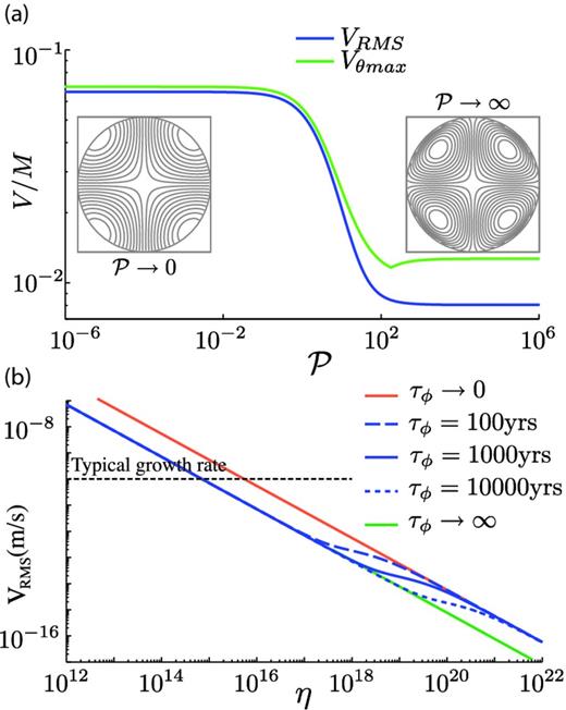
Analytic solution for Ra = 0. (a) Evolution of the dimensionless velocity as a function of the phase change number |$\mathcal {P}$|, with streamlines for |$\mathcal {P}\rightarrow 0$| (left) and |$\mathcal {P}\rightarrow \infty$| (right). The rms velocity and the maximum of the horizontal velocity are plotted. (b) Evolution of the rms velocity as a function of η, with velocity in m s−1. Except for the viscosity and the phase change time scale τϕ, the parameters used for definition of |$\mathcal {P}$| and M are given in Table 1. The kink in the curves corresponds to the change in regime between large |$\mathcal {P}$| (low viscosity) and low |$\mathcal {P}$| (large viscosity), and the corresponding viscosity value is a function of the phase change timescale τϕ.
In the limit |$\mathcal {P}\ll 1$|, corresponding to permeable boundary conditions, the streamlines of the flow cross the ICB, which indicates significant melting and freezing at the ICB. In contrast, the streamlines in the limit |$\mathcal {P}\gg 1$| are closed lines which do not cross the ICB, which indicates negligible melting or freezing at the ICB. The velocity is proportional to the effective Hartmann number M whereas the |$\mathcal {P}$| dependence is more complex. The velocities reaches two asymptotic values for low and large |$\mathcal {P}$| values, separated by a sharp kink. The discontinuity in the derivative of the maximum horizontal velocity slightly above |$\mathcal {P}\sim 10^2$| corresponds to a change of the spatial position of the maximum, when the streamlines become closed and the maximal horizontal velocity is obtained at the top of the cell and no longer at its bottom. The change of behaviour of the boundary from permeable to impermeable induces a significant decrease of the strength of the flow, since the velocity magnitude in the |$\mathcal {P}\gg 1$| regime is one order of magnitude smaller than when permeable boundary conditions (|$\mathcal {P}\ll 1$|) are assumed.
Fig. 2(b) shows the maximum of the velocity, now given in m s−1, as a function of the viscosity, using typical values of the parameters given in Table 1 and five different values for the phase change timescale τϕ, from zero to infinite. In term of dimensionless parameters, a high viscosity corresponds to small Hartmann number M and phase change number |$\mathcal {P}$|. Changing the timescale τϕ translates the position of the transition between the two regimes, the viscosity value corresponding to the transition being proportional to τϕ, but does not change the general trend of the curve, which is a linear decrease of the velocity magnitude in log-log space, except for the kink between the two regimes. The linear decrease is due to the viscosity dependence of the Hartmann number M ∝ η−1. For typical values of the phase change timescale between 100 and 10 000 yr, the kink between the two regimes occurs at a viscosity in the range 1017−1021 Pa s.
Typical values for the parameters used in the text, and typical range of values when useful.
| Parameter | Symbol | Typical value | Typical range |
|---|---|---|---|
| Magnetic field | B0 | 3 × 10⁻³ T | 10−1–10−3 T |
| Thermal diffusivitya | κT | 1.7 × 10⁻⁵ m2 s | 0.33–2.7 × 10⁻⁵ m2 s |
| Chemical diffusivityb | κχ | 10−10 m2 s | 10−10–10−12 m2 s |
| Viscosity | η | 1016 Pa s | 1012–1021 Pa s |
| Age of IC | τic | 0.5 Gyr | 0.2–1.5 Gyr |
| Density stratification (thermal case)c | ΔρT | 6 kg m−3 | 0.5–25 kg m−3 |
| Density stratification (compositional case)d | ΔρC | 5 kg m−3 | 1–10 kg m−3 |
| Phase change timescale | τϕ | 103 yr | 102–104 yr |
| Inner core radiuse | ric(τic) | 1221 km | |
| Acceleration of gravity (r = ric) | gic | 4.4 m s−2 | |
| Density of the solid phasee | ρ | 12 800 kg m−3 | |
| Density difference at the ICB | δρic | 600 kg m−3 | |
| Thermal expansivity | α | 10−5 K−1 | |
| Permeability | μ0 | 4π × 10−7 H m−1 |
In what follows, we will focus on the conditions which are the most favourable to deformation due to the poloidal component of the Lorentz force, and therefore focus on the case of low viscosity and large |$\mathcal {P}$|. The ICB would act as a permeable boundary only if |$\mathcal {P}\lesssim 10^{2}$| (see Fig. 2), corresponding to η ≳ 1017 Pa s. Under these conditions, the typical flow velocity would be ≲10−12 m s−1, that is two orders of magnitude or more smaller than the inner core growth rate, and would be unlikely to result in significant texturing. For this reason, we will let aside the high viscosity/low |$\mathcal {P}$| regimes to focus on low viscosity/high |$\mathcal {P}$| cases, for which the ICB acts as an impermeable boundary. This gives boundary conditions very different from previous studies, where perfectly permeable boundary conditions were assumed (Karato 1999; Buffett & Bloxham 2000). In particular, this implies that the flow velocity estimated by (Karato 1999) was overestimated by one order of magnitude.
According to eq. (36), the parameter |$\mathcal{P}$| varies linearly with time, which means that |$\mathcal {P}$| must have been small early in inner core's history. However, this is true for a very short time, when the inner core radius was very small, of the order |$r_{ic}(\tau _{ic})/\mathcal {P}_{0}^{1/2}$|, and this episode is unlikely to have observable consequences in the present structure of the inner core.
3.2 Zero growth rate
We first investigate the effect of the Lorentz force without taking into account the secular growth of the inner core (Pe = 0). Fig. 3 shows the vorticity and temperature fields obtained for different values of the Rayleigh number, at a given effective Hartmann number M = 104, for a thermally stratified inner core.
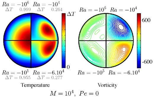
Snapshots of meridional cross-section of the temperature and the vorticity fields for M = 104 and a constant inner core radius, for four different values of the Rayleigh number (from top right, going clockwise: Ra = −104, −6 × 10⁴, −105, −106). When the stratification is large enough (Ra = −106), the flow is confined at the top of the inner core and the temperature field has a spherical symmetry. When the stratification is weak (Ra = −104), the flow is similar to the one in Fig. 2 for Ra = 0 and the temperature is almost uniform. The vorticity is scaled by |$\kappa _T /r_{ic}^2$| and the temperature by |$Sr^2_{ic}/6\kappa _T$|. For uic = 0, |$Sr^2_{ic}/6\kappa _T$| reduces to Ts(0) − Ts(ric).
When the Rayleigh number is small, the vorticity field is organized in two symmetric tores wrapped around the N-S axis.The stratification is too weak to alter the flow induced by the Lorentz force and the temperature field is advected and mixed by the flow. The velocity field is equal to the one calculated analytically for Ra = 0 (see Section 3.1 and Appendix D).
However, when the Rayleigh number is larger, the flow is altered by the stratification and is confined in an uppermost layer, as found by Buffett & Bloxham (2000). The velocity is smaller than in the case of neutral stratification. The temperature field is strongly stratified and the perturbations due to radial advection are small. The flow obtained here is similar to the flow induced by differential inner core growth with a stable stratification (Deguen et al.2011), with a notable difference: we impose a large |$\mathcal {P}$| implying a near zero radial flow vr across the ICB, whereas Deguen et al. (2011) impose a given vr as the driving force. The confinement of the flow in a thin layer is likely to concentrate the deformation and thus we may expect higher strain rates for a highly stratified inner core, but a different spatial distribution of the deformation.
To explore the parameter space in terms of Rayleigh and effective Hartmann numbers, we computed runs with Rayleigh numbers from −103 to −107 and effective Hartman number from 100 to 106. The maximum velocity (normalized by M) is plotted in Fig. 4 as a proxy to determine the regime. The largest velocity coincides with the flow velocity obtained for neutral stratification. The vorticity field corresponding to some of the points in the regime diagram are also shown in Fig. 4.
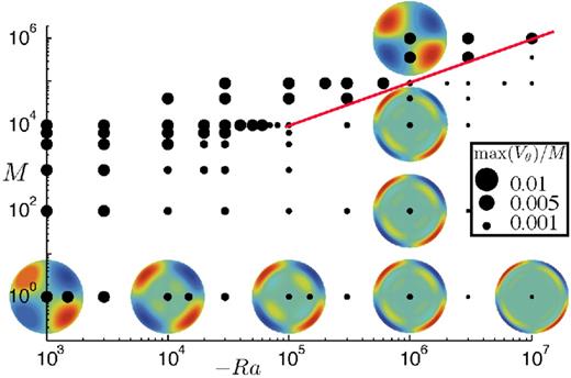
Maximum velocity (normalized by the Hartmann number M) in the upper vorticity layer, for a zero growth rate. The velocity is scaled by the diffusion velocity κ/ric. The maximum size of the dots corresponds to the value for Ra = 0 computed analytically. For some values of (M, −Ra), the vorticity field is plotted in the meridional cross section. The red line with a slope of 1 shows the limit between the two regimes.
The systematic exploration of the parameter space reveals two different dynamical regimes, which domains of existence in a (−Ra,M) space are shown in Fig. 4. In the upper left part of the diagram (large effective Hartmann number, low Rayleigh number), the flow is very similar (qualitatively and quantitatively) to the analytical solution for a neutral stratification, and deformation extends deep in the inner core. This regime is characterized by a negligible effect of the buoyancy forces, and will therefore be referred to as the weakly stratified regime. In the lower right part, the flow is confined in a shallow layer which thickness depends on the Rayleigh number only (not on M) and in which the velocity is smaller than for neutral stratification. This regime will be referred to as the strongly stratified regime.
3.3 Growing inner core
To investigate the effect of inner core growth, we compute several runs with a given set of parameters (Ra0, M0, Pe0), with the time t between t = 0.01 and t = 1. Unlike in Sections 3.1 and 3.2, the dimensionless numbers evolve with time, as described by eqs (19) to (22).
Fig. 5 shows the evolution of the vorticity field in six simulations, for a thermal stratification, with the same Rayleigh and effective Hartman numbers, RaT0 = −106, MT0 = 104, but different values of the Péclet number, which corresponds to increasing diffusivity from left to right. For each run, snapshots of the vorticity field corresponding to four time steps are shown, from top-right and going clockwise.
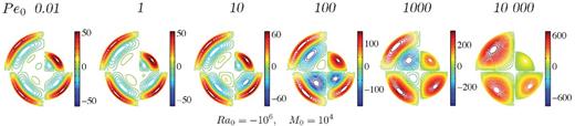
Snapshots of the vorticity field for simulations with dimensionless parameters M0 = 104, Ra0 = −106 and Pe0 = 0.01, 1, 10, 102, 103 and 104 (from left to right), with ric ∝ t1/2. Each panel corresponds to one simulation, with four time steps represented: t = 0.25, 0.50, 0.75 and 1 dimensionless time, from top-right and going clockwise. See Fig. 8 for strain rates of corresponding runs.
Fig. 5 shows that the thickness of the upper layer increases with increasing Péclet number. The transition between the two regimes of strong and weak stratification is shifted towards larger Rayleigh numbers when the Péclet number is increased. At low or moderate Péclet numbers (Pe0 ≤ 102 in the cases presented here), the magnitude of vorticity is almost constant time, implying that the deformation rate in the uppermost layer is also constant.
4 SCALING LAWS
In this section, we determine scaling laws for the thickness of the shallow shear layer and the maximum velocity in the layer in the strongly stratified regime from the set of equations developed in Section 2. We will first discuss the transition between the strongly stratified and weakly stratified regimes discussed in Fig. 4. We will then focus on the strongly stratified regime and estimate the deformation in the uppermost layer. Thermal and compositional stratification are discussed separately. The flow in the weakly stratified regime is given by the analytical model discussed in Section 3.1 and Appendix D for neutral stratification.
4.1 Balance between magnetic forcing and stratification
The effect of the stratification is negligible if the buoyancy forces, which are ∼−Raχ′, cannot balance the Lorentz force, which is ∼M. Since χ′ is necessarily smaller than |$|\bar{\chi }(r_{ic}) - \bar{\chi }(0)|$|, which by construction is equal to 1, the effect of the stratification will therefore be negligible if M ≫ −Ra. This is consistent with the boundary between the two regimes found from our numerical calculations, as shown in Fig. 4, as well as with the results of Buffett & Bloxham (2000) who found that the Lorentz force can displace isodensity surfaces by ∼ricM/(−Ra). This estimate is valid for both a growing or nongrowing inner core.
4.2 Scaling laws in the strongly stratified regime
Three of these terms depend on the growth rate: ξ∂χ′/∂t, Pe r · ∇χ′, and |$\xi \, \dot{\Delta \rho }/\Delta \rho \chi ^{\prime }$|. With our assumption of ric ∼ t1/2, we have ξ = 2Pe t and thus ξ ≲ Pe. Thus, the largest term among the growth rate-dependent terms is Pe r · ∇χ′ ∼ Pe χ′/δ.
4.2.1 Small Pe limit
4.2.2 Large Pe limit
Two conditions have to be fulfilled for these scaling laws to be valid. First, we must have Pe ≪ 1/δ, which is Pe ≫ (−Ra)1/6 using eq. (51). Also, we have assumed that the upper layer is thin (δ ≪ 1) and that the horizontal advection is small compared to the vertical one.
4.2.3 Time dependence
Our derivation does not make any assumption on the form of the inner core growth ric(t), and the scaling law validity should not be restricted to the ric(t) ∝ t1/2 case assumed in the numerical simulations.
4.3 Comparison with numerical results
Fig. 6 shows the thickness of the uppermost vorticity layer and the maximum horizontal velocity obtained in numerical simulations with a constant inner core radius, which corresponds to the small Péclet number limit. When −Ra/M ≪ 1, the flow has the geometry and amplitude predicted by our analytical model for Ra = 0. When −Ra/M ≳ 10 and the thickness of the upper layer is smaller than ≃0.3, the data points align on straight lines in log-log scale, with slopes close to the predictions of the scaling laws developed in Section 4.2.1 (eqs 47 and 48).
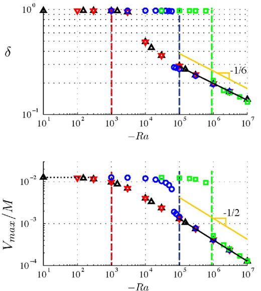
Results from simulations with a constant inner core radius. Evolution of the thickness of the uppermost vorticity layer (a) and maximum horizontal velocity (b) with the absolute value of the Rayleigh number −Ra. Colours correspond to different values of the effective Hartmann number M, and dashed lines to the corresponding −Ra = 10 M line. The velocity has been scaled with the effective Hartman number and the extreme value for low −Ra corresponds to the analytical model with no stratification (black horizontal dotted line). The solid black lines are the best fit for δ < 0.3, δ = 1.81(−Ra)−0.16 ± 0.013 and Vmax = 0.44M(−Ra)0.506 ± 0.002. The orange lines show the slopes predicted in Section 4.2.1.
Fig. 7 shows the vorticity layer thickness and maximum velocity as functions of Pe/(−Ra), in log-log scale, for runs in the large Péclet limit. The thickness of the upper layer and the maximum velocity align on slopes close to the 1/5 and 3/5 slopes predicted in Section 4.2.2. Fig. 7 has been constructed from runs with M = 1, but we have checked that, as long as the condition −Ra ≫ M is verified, the geometry of the flow does not depend on M and that the velocity is proportional to M.
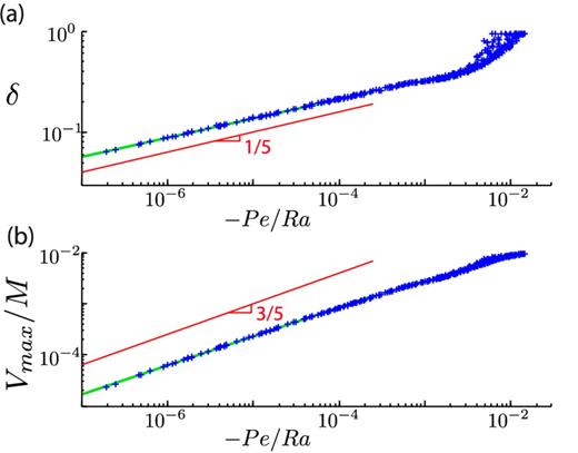
Thickness of the uppermost vorticity layer (a) and maximum velocity (b) as functions of −Pe/Ra. 50 runs are plotted, with Ra0 from −3 × 10³ to −1010 and Pe0 from 13 to 5000, with 10 time steps for each runs, and filtered by Pe0 ≫ 1/δ. Solid green lines are the best fit for δ < 0.25, which is δ = 1.24 (−Pe/Ra)0.192 ± 0.04 and Vmax = 0.143 M (−Pe/Ra)0.56 ± 0.09. The red lines are expected scaling laws developed in Section 4.2.2.
5 STRAIN RATE
Fig. 8 shows the von Mises equivalent strain rate for the runs corresponding to Fig. 5, highlighting regions of high deformation. The von Mises equivalent strain rate is the second invariant of the strain rate tensor, measuring the power dissipated by deformation (Tome et al.1984; Tackley 2000; Wenk et al.2000). Comparing Figs 5 and 8, we see that the deformation and vorticity fields have a similar geometry when the flow is organized in several layers, whereas the location of the regions of high deformation and high vorticity differ when the effect of stratification is small and the flow is organized in one cell only. In this case, which is similar to that studied by Karato (1999), the maximum deformation is at the edges of the cells, whereas in the case of large stratification, the strain is confined in the uppermost layer. In the strongly stratified regime, the deformation can be predicted from the scaling laws discussed in Section 4.2, as |$\dot{\epsilon }\sim u/\delta$| in dimensionless form, or |$\dot{\epsilon }\sim u\kappa /\delta r_{ic}^2$| in dimensional form.
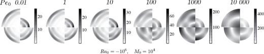
Snapshots of the von Mises equivalent strain rate for simulations with dimensionless parameters M0 = 104, Ra0 = −106, and Pe0 = 0.01, 1, 10, 102, 103 and 104 (from left to right), with ric ∝ t1/2. Each panel corresponds to one simulation, with four time steps represented : t = 0.25, 0.50, 0.75 and 1 dimensionless time, from top-right and going clockwise. See Fig. 5 for plots of the vorticity field of corresponding runs.
These scaling laws give upper bounds for the actual strain rate in the inner core, which evolves with time because of the time dependence of the parameters. The quantity |$1/\dot{\epsilon }$| is the time needed to deform the shear layer to a cumulated strain ∼1.
A more elaborated method of estimating ϵ is discussed in Appendix E. The results are close to what eq. (57) predicts for r > 0.3 ric(τic), but are more accurate for smaller r. The validity of both estimates is restricted to conditions under which the strong stratification scaling laws applies, which requires that M ≪ −Ra. This is only verified if the inner core radius is larger than ric(τic)(M0/Ra0)1/4 ≃ 0.02 ric(τic) in the thermal case, and ric(τic)(M0/Ra0)1/5 ≃ 0.07 ric(τic) in the compositional case.
6 APPLICATION TO THE INNER CORE
Typical values of the dimensionless parameters discussed in the text for the present inner core, using typical values from Table 1.
| Dimensionless parameter | Symbol | Thermal | Compositional |
|---|---|---|---|
| Rayleigh number | Ra | |$\frac{10^{16}\,{\rm Pa\,s}}{\eta }\times (-2.8 \times 10^8)$| | |$\frac{10^{16}\,{\rm Pa\,s}}{\eta }\times ( {-8 \times 10^{12}})$| |
| Effective Hartmann number | M | |$\left( \frac{B_0}{3\times 10^{-3}\,{\rm T}}\right)^2 \frac{10^{16}\,{\rm Pa\,s}}{\eta } \times {63}$| | |$\left( \frac{B_0}{3\times 10^{-3}\,{\rm T}}\right)^2 \frac{10^{16}\,{\rm Pa\,s}}{\eta } \times {1.07\times 10^7}$| |
| Péclet number | Pe | 2.8 | 4.7 × 10⁵ |
| Phase change number | |$\mathcal {P}$| | |$\frac{10^{16}\,{\rm Pa\,s}}{\eta }\times {10^4}$| | |$\frac{10^{16}\,{\rm Pa\,s}}{\eta } \times {10^4}$| |
See the definitions of the dimensionless parameters in the text.
If the stratification is of thermal origin, the Péclet number is on the order of 1 (Pe0 = 2.8). Fig. 5 shows that the low Péclet number scaling laws still agree reasonably well with the numerical results for Péclet numbers around 1; the low Péclet number scaling laws can therefore be used to predict the flow geometry and strength in the thermal stratification case. If the stratification is of compositional origin, the Péclet number is large (Pe0 ∼ 105) and thus the large Péclet limit scaling laws apply.
Estimates of the thickness of the upper layer, of the maximum velocity in this layer and of the expected strain rate are given in Table 3, using values of parameters of Tables 1 and 2. Because the viscosity is poorly known, we express these estimates as functions of the viscosity. As an example, assuming a viscosity of 1016 Pa s gives a shear layer thickness of 94 and 60 km in case of thermal and compositional stratification. The velocity in this layer is expected to be several orders of magnitude lower than the growth rate, and instantaneous deformation due to this flow is small: the typical timescale for the deformation is of order 102 Gyr for both cases, for η = 1016 Pa s. These values are obtained for the present inner core, which means it is the deformation timescale for the present uppermost layer. The deformation ϵ ∼ u/Pe is a decreasing function of the radius, and thus is higher in depth: compared to below the ICB, the strain at r = 0.5 ric is multiplied by 2 for thermal stratification, and by 4.6 for compositional stratification.
Estimates of the thickness, maximal horizontal velocity and strain rate of the upper layer for thermal stratification (low Pe) and compositional stratification (large Pe).
| Thermal stratification, low Péclet | Compositional stratification, large Péclet | |
|---|---|---|
| Thickness δ | |$\left( \frac{\eta }{10^{16}\,\mathrm{Pa\,s}}\right) ^{1/6}\times 94$| km | |$\left( \frac{\eta }{10^{16}\,\mathrm{Pa\,s}}\right) ^{1/5}\times 60$| km |
| Maximal horizontal velocityau | |$\left( \frac{10^{16}\,\mathrm{Pa\,s}}{\eta }\right) ^{1/2} \times 2.2\times 10^{-14}\,$|m s−1 | |$\left( \frac{10^{16}\,\mathrm{Pa\,s}}{\eta }\right) ^{2/5} \times 0.9\times 10^{-14}\,$|m s−1 |
| Instantaneous strain rateb|$\dot{\epsilon }$| | |$\left( \frac{10^{16}\,\mathrm{Pa\,s}}{\eta }\right) ^{2/3} \times 7.4\times 10^{-12}\,$| yr−1 | |$\left( \frac{10^{16}\,\mathrm{Pa\,s}}{\eta }\right) ^{3/5} \times 4.8\times 10^{-12}\,$| yr−1 |
| Strain ϵ = u/Pe | |$\left( \frac{10^{16}\,\mathrm{Pa\,s}}{\eta }\right) ^{1/2} \frac{r_{ic}}{r} \times 5.6 \times 10^{-4}$| | |$\left( \frac{10^{16}\,\mathrm{Pa\,s}}{\eta }\right) ^{2/5} \left( \frac{r_{ic}}{r}\right) ^{11/5} \times 2.4\times 10^{-4}$| |
aThis value has to be compared with a typical value for the growth rate: uic(τic) ≈ 10−11m s−1.
bAt t = τic.
As can be seen in eqs (55) and (56), the strain rate in the shear layer is a decreasing function of the stratification strength. This is the opposite of what Deguen et al. (2011) found in the case of a flow forced by heterogeneous inner core growth (Yoshida et al.1996). The flow geometry is similar to what has been found here if the inner core is stably stratified, with a shear layer below the ICB in which deformation is localized, but, contrary to the case of the Lorentz force, the strength of the flow and strain rate increase with the strength of the stratification. This difference is due to the fact that the velocity is imposed by the boundary conditions at the ICB in the case of heterogeneous inner core growth case, and therefore does not decrease when the stratification strength is increased. In contrast, the velocity in the shear layer produced by the Lorentz force depends on a balance between the Lorentz force and the viscous forces, and decreases with increasing stratification strength.
Using the method in Appendix E to estimate the strain, the deformation is found to be two orders of magnitude larger close to the centre of the inner core than at the edge. This means a nonnegligible strain for viscosity lower than 1012 Pa s.
The uppermost layer has a different behaviour because it does not have enough time to deform. This could stand for an isotropic layer at the top of the inner core, as observed by seismic studies. We expect this layer to be of the order of one hundred kilometres thick for thermal or compositional stratification.
7 CONCLUSION AND DISCUSSION
Following previous studies (Karato 1999; Buffett & Wenk 2001), we have developed a complete model for evaluating the deformation induced by the Lorentz force in a stratified inner core, investigating the effect of boundary conditions and neutral and strong stratification in the case of thermal or compositional stratification.
Calculating the flow for neutral stratification with different mechanical boundary conditions, we show that the boundary conditions depend on the values of the viscosity. If the viscosity is low, the ICB acts as an impermeable boundary, with no radial flow across the ICB, whereas if the viscosity is large the ICB acts as a permeable boundary, with fast melting and solidification at the ICB. We find that the velocity is larger than the inner core growth rate if the viscosity is lower than 1016 Pa s. Unlike previous studies, the boundary conditions assumed here are of impermeable type.
If the inner core has a stable density stratification, then we find that the stratification strongly alters the flow induced by the poloidal component of the Lorentz force. The deformation is concentrated in a thin shear layer at the top of the inner core, which thickness does not depend on the magnetic field strength, but depends on both the density stratification and the Péclet number, which compares the timescales of inner core growth and diffusion.
However, the deformation rate in this regime is predicted to be too small for producing significant LPO in most of the inner core, unless the inner core viscosity is smaller than 1010–1012 Pa s. The cumulated deformation can be two orders of magnitude larger close to the centre of the inner core, but remains smaller than 1 if the inner core viscosity is larger than 1012 Pa s.
We have made a number of simplifying assumption, but relaxing them is unlikely to significantly alter our conclusions. Our estimated values of the deformation are probably upper bounds. The effective strain in the inner core induced by the poloidal Lorentz force is expected to be even smaller than these values. Indeed, we use assumptions that maximize the strain rate in the inner core.
The geometry and strength of the magnetic field have been chosen to maximize the effect of the Lorentz force: the degree (2,0) penetrates deeper in the inner core than higher orders (smaller length-scales) and is less likely to vary with time. The smaller scale components of the magnetic field vary on a shorter timescale, which make them more sensitive to skin effect.
We have assumed the magnetic field to be time-independent, a reasonable assumption because the fluctuations associated with outer core dynamics occur on a timescale short compared to the timescale of inner core dynamics. The evolution of the magnetic field strength on the timescale of inner core growth is poorly constrained, but seems unlikely to have involved order of magnitude variations.
Though a growth law of the form ric ∝ t1/2 has been assumed in the numerical simulations, our derivation of the scaling laws (Section 4.2) makes no assumption on the inner core growth law, and our scaling law should therefore also apply if this assumption is relaxed.
We would like to thank two anonymous reviewers for their constructive comments, and Christie Juan for her help at a preliminary stage of this project. RD gratefully acknowledges support from grant ANR-12-PDOC-0015-01 of the ANR (Agence Nationale de la Recherche). SL was supported by the Institut Universitaire de France for this work.
REFERENCES
APPENDIX A: POLOIDAL/TOROIDAL DECOMPOSITION
A1 Momentum equation using poloidal decomposition
A2 Poloidal decomposition of the boundary conditions
APPENDIX B: THERMAL STRATIFICATION
We derive here the expression of the reference diffusive potential temperature profile given in eq. (24), under the assumption of ric ∝ t1/2.
APPENDIX C: COMPOSITIONAL STRATIFICATION
The source term Sc of the conservation of light elements is directly related to the evolution of the concentration of light elements in the solid that freezes at the ICB |$\dot{c}_{ic}^s(t)$|. Following Gubbins et al. (2013) and Labrosse (2014), this term depends both on the evolution of the concentration in the liquid outer core, which increases when the inner core grows because the solid incorporates less light elements than is present in the outer core, and on the evolution of the partition coefficient between solid and liquid.
In this paper, we will focus on the simplest case for which the partition coefficient does not depend on temperature or concentration. Thus, the concentration in the solid is increasing with the radius of the inner core, as the concentration in the liquid increases. This will promote a stably stratified inner core, whereas Gubbins et al. (2013) and Labrosse (2014) focused on the potentially destabilizing effects of variations of the partition coefficient.
APPENDIX D: ANALYTIC SOLUTION FOR NEUTRAL STRATIFICATION
We solve eq. (A8) for a neutral stratification, Ra = 0, with the boundary conditions (A13) and (A14) described in section (A2).
Except for (l = 2, m = 0), |$p_l^m=0$| is solution of the eq. (D1) and verifies the boundary conditions (A13) and (A14).
From eqs (D7) and (D8), we obtain the maximum absolute value of the horizontal velocity and the rms velocity that are shown on Fig. 2. Both graphs have a sigmoid shape, and thus we are mostly interested in the extreme values for each velocity, which are given in Table D1.
Extreme values for rms velocity and maximum of the absolute value of the horizontal velocity for two extreme values of |$\mathcal {P}$|. Velocities are proportional to M and thus only the value v/M is given.
| |$\mathcal {P}\rightarrow 0$| | |$\mathcal {P}\rightarrow \infty$| | |
|---|---|---|
| Vrms/M | 0.06609 | 0.00805 |
| max |uθ(r, θ)|/M | 0.06944 | 0.01270 |
| |$\mathcal {P}\rightarrow 0$| | |$\mathcal {P}\rightarrow \infty$| | |
|---|---|---|
| Vrms/M | 0.06609 | 0.00805 |
| max |uθ(r, θ)|/M | 0.06944 | 0.01270 |
APPENDIX E: INTEGRATION OVER TIME OF THE DEFORMATION
E1 General discussion
This equation leads to simple forms at the low and large Péclet limits, with ϵ ∝ t−1/2 for thermal stratification and low Péclet, and ϵ ∝ t−11/10 for compositional stratification and large Péclet. In what follows, we will compare the simple estimate given above with results of more elaborate calculations.
The estimations of |$\dot{\epsilon }_{vM}$| depend on the scaling laws defined in Section 5, and also on the time dependence of the parameters we have defined.
E2 Low Pe—Thermal stratification
The strain rate is assumed to be constant over the layer δ whereas we could have used numerical results of the simulations to have the exact repartition and profile of strain over radius and time. But because the von Mises strain rate profile over radius is close to a rectangular function, it is easier to work with an analytic solution such as the one discussed here. It implies a linear increase of the absolute value of the strain, which is unlikely. This will in general overestimate the total strain.
Comparison between the strain computed from (E13) and the simplest solution u/Pe discussed in the text is plotted on Fig. E1. The solution u/Pe is a good approximation for radius larger than 0.3 τic, except in the uppermost layer, in which the deformation did not occur completely yet. It is interesting to notice that this magnetic forcing is expected to be several orders of magnitude more efficient when the inner core was younger.
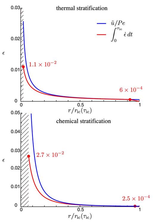
Strain as a function of the radius of the inner core for thermal stratification (a) and compositional stratification (b). Integration from eq. (E4) is the red line (analytical solution for thermal stratification and numerical solution for compositional stratification), and the blue lines stand for the estimation u/Pe, which is valid for r > 0.5 ric. The minimum radius is computed for Ra/M = 1, limit under which the strong stratification approximation is no longer valid.
E3 Large Pe—Compositional stratification
No exact solution for inverting ric(τic)(tmax/τic)1/2 − δ(τic)(t/τic)−1/5 = r can be found. Fig. E1(b) shows the strain rate according to numerical integration and the approximation u/Pe. u/Pe is a good approximation for r > 0.3 ric.
