


Abstract
Computationally efficient 3-D frequency-domain full waveform inversion (FWI) is applied to ocean-bottom cable data from the Valhall oil field in the visco-acoustic vertical transverse isotropic (VTI) approximation. Frequency-domain seismic modelling is performed with a parallel sparse direct solver on a limited number of computer nodes. A multiscale imaging is performed by successive inversions of single frequencies in the 3.5–10 Hz frequency band. The vertical wave speed is updated during FWI while density, quality factor QP and anisotropic Thomsen's parameters δ and ϵ are kept fixed to their initial values. The final FWI model shows the resolution improvement that was achieved compared to the initial model that was built by reflection traveltime tomography. This FWI model shows a glacial channel system at 175 m depth, the footprint of drifting icebergs on the palaeo-seafloor at 500 m depth, a detailed view of a gas cloud at 1 km depth and the base cretaceous reflector at 3.5 km depth. The relevance of the FWI model is assessed by frequency-domain and time-domain seismic modelling and source wavelet estimation. The agreement between the modelled and recorded data in the frequency domain is excellent up to 10 Hz although amplitudes of modelled wavefields propagating across the gas cloud are overestimated. This might highlight the footprint of attenuation, whose absorption effects are underestimated by the homogeneous background QP model (QP = 200). The match between recorded and modelled time-domain seismograms suggests that the inversion was not significantly hampered by cycle skipping. However, late arrivals in the synthetic seismograms, computed without attenuation and with a source wavelet estimated from short-offset early arrivals, arrive 40 ms earlier than the recorded seismograms. This might result from dispersion effects related to attenuation. The repeatability of the source wavelets inferred from data that are weighted by a linear gain with offset is dramatically improved when they are estimated in the FWI model rather than in the smooth initial model. The two source wavelets, estimated in the FWI model from data with and without offset gain, show a 40 ms time-shift, which is consistent with the previous analysis of the time-domain seismograms. The computational efficiency of our frequency-domain approach is assessed against a recent time-domain FWI case study performed in a similar geological environment. This analysis highlights the efficiency of the frequency-domain approach to process a large number of sources and receivers with limited computational resources, thanks to the efficiency of the substitution step performed by the direct solver. This efficiency can be further improved by using a block-low rank version of the multifrontal solver and by exploiting the sparsity of the source vectors during the substitution step. Future work will aim to update attenuation and density at the same time of the vertical wave speed.
1 INTRODUCTION
Today, the most widespread implementation of full waveform inversion (FWI) is performed in the time domain. This mainly results because the evolution problem underlying time-domain modelling is versatile enough to tackle a wide range of applications involving different problem sizes, wave physics and acquisition geometries in controlled-source exploration geophysics and earthquake seismology (e.g. Komatitsch et al.2002; Peter et al.2011; Fichtner et al.2013; Vigh et al.2013; Warner et al.2013a; Vigh et al.2014b; Stopin et al.2014; Borisov & Singh 2015; Zhu et al.2015). However, the computational cost of time-domain FWI scales to the number of sources, which makes these approaches computationally demanding when several thousands of seismic sources generated by 3-D modern wide-azimuth surveys should be processed. The elapsed time required to perform time-domain FWI applications is conventionally reduced by distributing the seismic sources over the processors of parallel computers. This parallel strategy requires huge computational platforms, in particular if this source parallelism is combined with a second level of parallelism by domain decomposition of the computational mesh (Etienne et al.2010). These computational resources can be reduced by limiting the number of sources during FWI iterations by random source subsampling over FWI iterations (van Leeuwen & Herrmann 2012; Warner et al.2013a), plane-wave source blending (Vigh & Starr 2008) or source blending with random encoding (Krebs et al.2009; Schiemenz & Igel 2013). These strategies require increasing the number of FWI iterations and might damage the quality of the FWI results.
Alternatively, FWI can be performed in the frequency domain (e.g. Ravaut et al.2004; Brenders & Pratt 2007a,b; Plessix 2009; Plessix et al.2012) where seismic modelling reduces to a stationary boundary-value problem (Marfurt 1984). In this case, the computational cost of frequency-domain FWI is proportional to the number of discrete frequencies involved in the inversion. Whatever the linear algebra technique used to solve this boundary-value problem, namely, iterative or direct Gauss-elimination methods, it is acknowledged that the frequency-domain formulation is beneficial as long as the FWI can be limited to a few discrete frequencies.
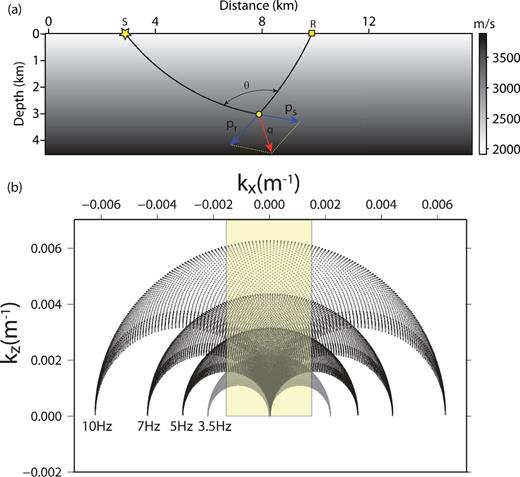
Resolution power of FWI and its relationship with the experimental setup. (a) The velocity linearly increases with depth in the subsurface. Two rays starting from the source S and the receiver R connects a diffractor point in the subsurface (yellow circle) with a scattering angle θ. The sum of the slowness vectors ps and pr, denoted by q, defines the orientation of the local wavevumber vector spanned at the diffractor position by this source–receiver pair. (b) Local wavenumber spectrum spanned by four discrete frequencies 3.5, 5, 7 and 10 Hz and a 16 km maximum offset fixed-spread acquisition at the diffractor position. These four frequencies are enough to map the shaded wavenumber area, which is assumed to be representative of the wavenumber spectrum of the subsurface target. The missing low wavenumber components are assumed to be embedded in the initial FWI model and can be ideally built by joint refraction and reflection tomography. See Mora (1989) for a more complete review.
In the frequency domain, seismic modelling consists of solving a linear system per frequency. This linear system relates the seismic source in the right-hand side to the monochromatic wavefields through a sparse impedance matrix, the coefficients of which depend on the frequency and the subsurface properties (Marfurt 1984). For 2-D problems, the linear system can be solved efficiently with sparse direct solver (Duff et al.1986). During a pre-processing stage, a lower–upper (LU) factorization of the impedance matrix is performed before computing the monochromatic wavefields by forward/backward substitutions for each right-hand side of the acquisition (e.g. Stekl & Pratt 1998). The LU factorization of the matrix generates some fill-ins (extra non-zero coefficients are added), making the LU factorization memory demanding. However, the solution step is quite computationally efficient and hence this approach is highly beneficial as long as a limited number of frequencies is processed with a large number of sources. Another key advantage of frequency-domain seismic modelling is the straightforward and cheap implementation of any kind of attenuation mechanism through the use of complex-valued wave speeds (Marfurt 1984), while the time domain implementation requires computation of additional memory variables during seismic modelling (e.g. Emmerich & Korn 1987; Carcione et al.1988; Robertsson et al.1994; Blanch et al.1995; Bohlen 2002; Kurzmann et al.2013; Groos et al.2014). Implementation of the inverse problem with attenuation (Tarantola 1988) is also simpler and more computationally efficient in the frequency domain for several reasons. First, the fact that the wave equation operator may not be symmetric in presence of attenuation does not introduce implementation difficulties to solve the adjoint equation in the frequency domain (one just needs to solve a system involving the transpose of the matrix instead of the matrix itself). Second, the expression of the complex-valued wave speed gives an explicit access to the physical parameter to be imaged, such as the quality factor, unlike in the time domain, which might require more complex manipulation (Kurzmann et al.2013; Fichtner & van Driel 2014; Groos et al.2014). Third, the reverse-time recomputation of the incident wavefield during the adjoint simulation in time-domain FWI is unstable in presence of attenuation, although some recent studies might have overcome this issue with pseudo-spectral modelling engines (Zhu 2015). Alternatively, this re-computation can be performed with check-pointing approaches, which might however be more computationally expensive (Symes 2007; Anderson et al.2012). Indeed, the re-computation of the incident wavefields during adjoint simulation is not necessary in the frequency domain because one or several incident monochromatic wavefields can be kept in memory all over the gradient computation.
For 3-D problems, the LU factorization has been considered for a long time intractable. This has prompted the development of hybrid approaches of FWI for which seismic modelling is performed in the time domain, while the inversion is performed in the frequency domain to manage compact volume of data (Nihei & Li 2007; Sirgue et al.2008, 2010). Alternatively, the time-harmonic wave equation can be solved with iterative solvers (Plessix 2007, 2009). This raises however two issues: The first one deals with the design of an efficient pre-conditioner of the system to make the iterative approach competitive with the time-domain one by making the number of iterations independent to the frequency; The second one is related to the efficient processing of multiple right-hand sides to make iterative approach competitive with the direct solver one. For a more exhaustive discussion on the pros and cons of different possible modelling approaches for FWI, the reader is referred to Virieux et al. (2009).
Despite the memory demand of the LU factorization, a feasibility analysis presented in Operto et al. (2007), Ben Hadj Ali et al. (2008) and Brossier et al. (2010) has shown that realistic problems can be efficiently tackled today with sparse direct solver in the acoustic approximation, at low frequencies (<10 Hz), in particular for fixed-spread acquisitions such as ocean bottom seismic ones. Since then, novel multifrontal methods, in which the so-called dense frontal matrices are represented with low-rank subblocks amenable to compression, have also reduced the cost of these approaches further in terms of memory demand, floating-point operations and volume of communication (Wang et al.2011; Weisbecker et al.2013; Amestoy et al.2015). Specific finite-difference stencils for visco-acoustic modelling have been designed to keep the memory demand of the LU factorization tractable (Jo et al.1996; Hustedt et al.2004; Operto et al.2007). As it is often mandatory to account for anisotropy in FWI, we recently extend such stencil to account for VTI anisotropy in the 3-D visco-acoustic modelling without generating significant computational overheads (Operto et al.2014). A suitable finite-difference stencil in terms of compactness and accuracy for frequency-domain modelling has been also designed for the 3-D elastic wave equation (Gosselin-Cliche & Giroux 2014), although the feasibility of representative applications of 3-D frequency-domain elastic modelling with direct solvers has still to be demonstrated.
This study presents the first application (to the best of our knowledge) of 3-D visco-acoustic vertical transverse isotropic (VTI) frequency-domain FWI based on sparse direct solver on a real ocean-bottom cable (OBC) data set from the North Sea, with the aim to discuss the pros and cons in terms of computational efficiency and reliability of this FWI technology. Seismic modelling is performed in the VTI visco-acoustic approximation but only the vertical wave speed is updated during FWI. The data set, which comprises 2302 receivers and 49 954 shots, has been recorded with a four-component OBC acquisition in the Valhall oil field (Barkved & Heavey 2003). Only the hydrophone component is considered in this study consistently with the acoustic approximation that is used during our imaging. The acquisition layout cover an area of 145 km2 and the maximum depth of the subsurface model is 4.5 km. Data are inverted in the 3.5–10 Hz frequency band.
We have processed the same data set as that presented in Sirgue et al. (2010). In Sirgue et al. (2010), isotropic (acoustic) seismic modelling is performed in the time domain, while the inversion is performed in the frequency domain within the 3.5–7 Hz frequency band. Although anisotropy was not taken into account to our knowledge, Sirgue et al. (2010) have shown impressive results. In particular, FWI reveals glacial channel system in the near surface whose image extends far beyond the cable layout as well as a very detailed image of a gas cloud with a complex network of short-scale low-velocity anomalies radiating out from it. We shall use these results as a reference to qualify the subsurface models obtained with our purely frequency-domain FWI method. Other applications of 3-D time-domain isotropic acoustic FWI on the Valhall data are also presented in Liu et al. (2013) and Schiemenz & Igel (2013).
The relevance of the acoustic approximation for FWI of marine data has been discussed in Barnes & Charara (2009). An analysis focused on the Valhall case study has shown that acoustic FWI of elastic wavefields recorded by the hydrophone component gives accurate P-wave velocity model (Brossier et al.2009). This results because the soft seabed in Valhall as well as relatively mild velocity contrasts compared to more complex geological environments involving salt, basalt or carbonate layers limit the amount of P-to-S conversions. The validity of the acoustic approximation in the Valhall environment was later on supported by an application of 2-D visco-acoustic multiparameter FWI on the hydrophone component of the Valhall OBC data set (Prieux et al.2011, 2013a). The resulting P-wave velocity, density and QP models were subsequently used as background models to perform elastic inversion of the hydrophone component in a first step followed by the elastic inversion of the geophone components in a second step, these two inversions being mainly devoted to the S-wave velocity model building (Prieux et al.2013b).
Warner et al. (2013a) have presented a real data case study performed in a similar geological context (North Sea) and for a similar OBC acquisition. In their study, both seismic modelling and FWI are performed in the time domain in the VTI acoustic approximation. A 3–6.5 Hz frequency band was processed, that is part of the frequency band processed in this study. Warner et al. (2013a) have discussed how acquisition subsampling is managed during FWI to reduce the computational burden of time-domain seismic modelling for multiple sources. We shall use this study as a reference to discuss the pros and cons of the frequency-domain approach in terms of computational efficiency. Another approach to reduce the computational burden of time-domain modelling, that is based on random source encoding rather than source subsampling, is presented in Schiemenz & Igel (2013).
In the first part of this study, we briefly review our implementation of frequency-domain seismic modelling and inversion. In the second part, we present the application of our FWI algorithm on the real data from Valhall. We first present the FWI results, which show geological features comparable to those shown in Sirgue et al. (2010) in the upper part of the target as well as well-focused deep reflectors below the reservoir level. Second, we discuss the relevance of the FWI results based on seismic modelling and source wavelet estimation. Then, we discuss the computational efficiency of our frequency-domain approach relative to ones based on time-domain modelling. In the Discussion section, we review the artefacts that might have been created by the mono-parameter nature of the reconstruction and by the wave physics approximations used in this study. In the Conclusion, we draw some generalizations from this case study and review the perspectives of this work in particular in terms of multiparameter FWI.
2 FREQUENCY-DOMAIN FWI: METHOD
We review the VTI visco-acoustic wave equation that is used for seismic modelling. The reader is referred to Operto et al. (2014) for more details. Then, we develop the expression of the gradient of the misfit function using the Lagrangian formulation of the adjoint-state method (Plessix 2006) and discuss some algorithmic aspects.
2.1 Forward problem
2.2 Inverse problem
2.2.1 Parallel algorithm
The optimization algorithm is implemented with a reverse-communication user interface (Dongarra et al.1995), which allows for a separation between the numerical optimization procedure and the specific physical application. This algorithm is described in more details in Métivier et al. (2013, 2014) and Métivier & Brossier (2015). The main inputs that must be provided by the user to the minimization subroutine are the current subsurface model, the misfit function computed in this model as well as its gradient. The main steps of the frequency-domain FWI gradient computation are reviewed in Algorithm 1. The first step consists of building the matrices A and B before the parallel factorization of A with the direct solver MUMPS. At this stage, the LU factors are stored in core memory in distributed form. Second, we perform a loop over np partitions of few tens of right-hand sides of the eqs (2) and (11). The incident and adjoint wavefields associated with each right-hand side of the partition are efficiently computed in parallel with MUMPS taking advantage of multithreaded BLAS3. The wavefield solutions for the incident and adjoint sources of the current source partition are recovered in core memory in distributed form: each message-passing interface (MPI) process manages a spatial subdomain of all the wavefields generated by the source partition. The underlying domain decomposition is driven by the distribution of the LU factors over the MPI processes and therefore is unstructured (Sourbier et al.2009). This domain decomposition makes the parallel computation of the gradient more complicated to implement as it would require point-to-point communication between the subdomains of the decomposition when the radiation pattern matrix ∂A/∂m is built and multiplied with the incident wavefields during the gradient computation (eq. 10). To perform the computation of the gradient in parallel, we rather favour a parallelism with respect to the sources at the expense of a parallelism by domain decomposition in order to have access on each MPI process to the wavefields on the entire computational domain. This prompts us to redistribute with a collective communication (MPI_ALLTOALLV) the wavefields over the MPI processes according to the right-hand side index in the partition. At the end of the loop over the right-hand side partitions, the gradient and the pre-conditioner contributions, that are distributed over the MPI processes, are centralized back on the master process with a collective communication (MPI_REDUCE) before the step length estimation performed by the optimization toolbox with a conventional line search, which guarantees that the Wolfe conditions are satisfied (Nocedal & Wright 2006). The computational cost of each step of the algorithm is discussed in more details in Section 3.4.
GRADIENT SUBROUTINE
| 1: | Build matrices A and B on master process |
| 2: | Parallel LU factorisation of A (MUMPS) |
| 3: | for|$i=1\, {\rm to} \, N_{p_{rhsp}}\, (p_{rhs}{:}\hbox{ partition of right-hand sides})$|do |
| 4: | Distributed build of b(i) (sources of the state equations) |
| 5: | Parallel computation of |$p_h^{(i)}$| with centralised in-core storage (MUMPS) |
| 6: | Infer |$p_v^{(i)}$| and p(i) from |$p_h^{(i)}$| |
| 7: | Sample p(i) at receivers, compute source signature(i) and Δd(i), and update C |
| 8: | Distributed build of |$\frac{1}{3} ({\bf{B}}^\dagger + 2 {\bf{I}}) R^t \Delta {\bf{d}}^{i}$| on master process (sources of the adjoint-state equations) |
| 9: | Parallel computation of |$ a_1^{(i)}$| with centralised in-core storage (MUMPS) |
| 10: | Distribute |$p_h^{(i)}$| and |$a_1^{(i)}$| over MPI processes .wrt. sources ∈ partition i |
| 11: | form = 1 to Mdo |
| 12: | Compute radiation pattern matrix ∂A/∂m |
| 13: | Distributed update of ∇mC and H |
| 14: | end for |
| 15: | end for |
| 16: | Centralise ∇mC and H |
| 17: | Scale ∇mC with H |
The complex-valued recorded data are stored in the frequency domain with the SEISMIC UNIX (SU) format. The data are sampled with a uniform frequency interval. The first frequency, the frequency interval and the number of frequencies are provided in the trace header at specific location. Indeed, the frequency-domain FWI has the necessary versatility to pick an arbitrary subset of frequencies in the recorded data to perform inversion.
3 APPLICATION TO VALHALL
3.1 Geological context, seismic acquisition and starting models
3.1.1 Geological context
The Valhall oil field is a giant field located in the North Sea in 70 m of water. It is characterized by the presence of gas in the overburden, forming locally a gas cloud, that makes seismic imaging at the reservoir depths challenging. The over-pressured, under-saturated Upper Cretaceous chalk reservoir is located at 2.5 km depth and shows evidence of compaction during depletion, leading to subsidence in the overburden (Barkved et al.2010).
3.1.2 Seismic acquisition and data set
The layout of the 3-D wide aperture/azimuth acquisition is shown in Fig. 2(a). The targeted area covers a surface of 145 km2. A recording layout of 12 cables equipped with four-component receivers recorded 49 954 shots, located 5 m below the sea surface. The nominal distance between cables is 300 m, with the two outer cables at 600 m. The inline spacing between two consecutive shots and receivers is 50 m. The total number of receivers is 2302. In this study, we use only the data from the hydrophone component. We exploit the source–receiver reciprocity to process the hydrophone components as explosive sources and the shots as hydrophones sensors to reduce the number of forward modelling during FWI by one order of magnitude.
![(a) OBC acquisition layout. The ocean-bottom cables are denoted by red lines. The shot positions by black dots. Two receiver positions r1 and r2 at (X,Y) = (5.6 km, 14.5 km) and (X,Y) = (8021 m, 14 108 m), respectively, are denoted by circles. An horizontal slice of the gas cloud at 1 km in depth, that was obtained by FWI (this study), is shown in transparency to delineate its zone of influence. The star denotes the position of the well log. Positions of cable 13, 21 and 29 are labelled. (b) Reverse time migrated image with superimposed in transparency vertical wave speeds determined by reflection traveltime tomography. The sonic log is also shown by the black line [adapted from Prieux et al. (2011)].](https://oup.silverchair-cdn.com/oup/backfile/Content_public/Journal/gji/202/2/10.1093/gji/ggv226/2/m_ggv226fig2.jpeg?Expires=1716399403&Signature=i7MPnWb-a~m5g0nl0w~uDoLsp1HthJJqNE5PI8Pdifyid2QaHfYxl1PPpTHDJMpWsWnHXldbE5Z3VNrP6ysxseZM0-0xmKD3wK2NoqNeWWm5JyK0oCyVLEtnxfyrht6PXvjJapUnHxX4LkSJJ9ADlWkBNgNwAn9XLoDXFZoauzUj6o8jC9oLoehy4MpcILPql2CeYuXBhLZAfVEyZCCenzBAIF86JYK2wsDRIoQGZ3v5AjB6rs5iXHEC5J39BIghCp9ygWyBpSiy0uCYxabJzzl8dN0sRDapmtpdE-GfQtAD2dtqcXAk73eadWVx5eHb5croeU4G7MNxZFGI9Um04A__&Key-Pair-Id=APKAIE5G5CRDK6RD3PGA)
(a) OBC acquisition layout. The ocean-bottom cables are denoted by red lines. The shot positions by black dots. Two receiver positions r1 and r2 at (X,Y) = (5.6 km, 14.5 km) and (X,Y) = (8021 m, 14 108 m), respectively, are denoted by circles. An horizontal slice of the gas cloud at 1 km in depth, that was obtained by FWI (this study), is shown in transparency to delineate its zone of influence. The star denotes the position of the well log. Positions of cable 13, 21 and 29 are labelled. (b) Reverse time migrated image with superimposed in transparency vertical wave speeds determined by reflection traveltime tomography. The sonic log is also shown by the black line [adapted from Prieux et al. (2011)].
We superimpose on the acquisition layout a depth slice of the gas cloud (built by FWI in this study) to delineate its zone of influence (Fig. 2a). The star shows the position of a sonic log that will be used to locally check the relevance of our FWI results. The black circles show the position of two receivers, referred to as r1 and r2 in the following, whose data will be more specifically analysed in the sequel of this study. Fig. 2(b) shows a 2-D reverse time migrated section along cable |$\#21$|, which is located near the periphery of the gas cloud (Prieux et al.2011). This migrated image was computed in a vertical section of the 3-D subsurface VTI model that is used as the initial FWI model in this study (see next section). The migrated image shows a low-velocity zone between 1.5 and 2.5 km depth, which corresponds to the most extensive overburden gas charges in the tertiary section (Barkved et al.2010). In the following, we refer to as gas cloud an accumulation of gas above these levels between 1 and 1.5 km depth. The reservoir reflectors are at around 2.5–3.0 km depth (Barkved et al.2010). The migrated section also shows a deep reflector between 3 and 3.7 km in depth, that corresponds to the base of the cretaceous.
Seismograms recorded by receivers r1 and r2 are shown in Fig. 3 for the inline shot profile passing through the receiver positions. The receiver r1 belongs to the cable |$\#13$|, whose coincident inline shot profile passes through the gas cloud, while the receiver r2 belongs to cable |$\#29$|, which is located away from the gas cloud (Fig. 2a). The receiver gathers are shown without (top panels) and with (bottom panels) a linear moveout, which is equal to the absolute value of the source–receiver offset divided by a reduction velocity of 2.5 km s−1. In the second representation, diving waves and post-critical reflections are nearly horizontal, hence making the interpretation of the wide-angle arrivals easier. The reflected wavefield is dominated by a shallow reflection (red arrows), the reflection from the top of the low-velocity zone at 1.5 km depth (white arrows) and the reflection from the top of the reservoir at 2.5 km depth (black arrows). Solid arrows point on the pre-critical reflections, while the dash arrows points on the post-critical reflections (the critical distance associated with the reflection from the top of the reservoir is challenging to identify due to the interference with shingling multirefracted/converted waves from the sea bottom). Of note the critical distances of the reflections are smaller in Fig. 3(a) compared to Fig. 3(b). This highlights the fact that the presence of the gas cloud above 1.5 km depth decreases the average wave speed between the sea bottom and the 1.5 km depth.
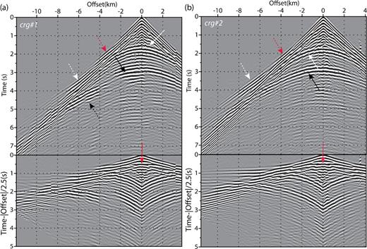
Time-domain common-receiver gathers for inline (Y) shot profile running across the receiver position. (a) Receiver r1. (b) Receiver r2. The data are plotted with a reduction velocity of 2.5 km s−1 on the bottom panel. The red, white, black arrows point on the reflection from a shallow reflector, the top of the low-velocity zone and the top of the reservoir, respectively. The solid arrow points on the pre-critical reflections, while the dashed ones points on the post-critical reflections. The critical distance is difficult to identify for the reflection from the top of reservoir because of the interference with multirefracted waves at the sea bottom.
The footprint of the gas cloud on the wavefield is manifested by the more discontinuous pattern of the reflection from the top of the reservoir in Fig. 3(a) compared to the one shown in Fig. 3(b). In particular, we note the bright critical reflection between −8 km and −4 km of offset (Fig. 3a, dash black arrow). The short-spread reflection wavefield (offsets −2 km to 2 km) is also more ringing between 1.5 and 3 s two-way traveltimes in Fig. 3(a) compared to Fig. 3(b). In Fig. 3, the first arrival also shows a more discontinuous en echelon pattern between −4 km and −7 km of offset that suggests an alternation of high-velocity and low-velocity layers, this pattern being absent in Fig. 3(b).
3.1.3 Starting FWI subsurface model
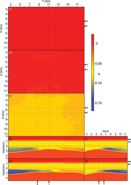
The vertical-velocity (V0) and the Thomsen's parameter models, which are used as initial models for FWI, were built by reflection traveltime tomography (courtesy of BP). Horizontal and vertical slices of the V0 model are shown in Fig. 4, while the corresponding slices of the η parameter show that the maximum anisotropy reaches a value of 16 per cent at the reservoir level (Fig. 5). The horizontal slice at 1 km depth and the inline vertical slice at X = 5.5 km pass through the gas cloud, which appears as a smooth low-velocity blob in the V0 model (Figs 4c and d). The accuracy of this starting model has been assessed in two dimensions along cable |$\#21$| in Prieux et al. (2011). In particular, Prieux et al. (2011) have shown that common-image gathers (CIGs) computed in this starting model exhibit fairly flat reflectors. 2-D FWI has improved the flatness of the reflectors in the CIGs in the shallow part of the subsurface, down to 1 km, and locally at the reservoir level [Prieux et al. (2011), their fig. 9, and Castellanos et al. (2015), their fig. 15]. Of note, the interface delineating the top of the reservoir is quite sharp in this starting model (see also Figs 2b and 6). In contrast to previous studies (Sirgue et al.2010; Warner et al.2013b), we did not smooth this starting model for FWI. The drawback might be that FWI will face difficulties to update this reflector if it is incorrectly positioned. The advantage may be that this sharp discontinuity will generate energetic reflected waves during the early iterations, whose downgoing and upgoing paths may help to update the long-to-intermediate wavelengths in the area of the model that are not covered by diving waves (namely, the low-velocity zone; Brossier et al.2015). This issue is illustrated by two 7 Hz monochromatic sensitivity kernels or wave paths (Woodward 1992) that have been, respectively, computed in the initial model shown in Fig. 4 and in a smoothed version of this initial model (Fig. 7). The smoothing has been performed with a 3-D Gaussian filter with a 500-m correlation length in the three Cartesian directions, roughly corresponding to the average wavelength at the 4 Hz frequency. The sensitivity kernel computed in the smoothed model (Fig. 7a) is dominated by the so-called migration isochrones below the penetration depth of diving waves, which will make challenging the update of the long wavelengths at these depths. Prieux et al. (2011) have shown from a 2-D analysis along cable |$\#21$| that, owing to the available offset range, the penetration depth of the diving waves is around 1.5 km and hence corresponds to the top of the low-velocity zone. This is qualitatively shown in Fig. 3 by the fact that the post-critical branch of the reflections from the top of the low-velocity zone becomes tangent to the diving waves at long offsets. Note, however, that accounting for the full 3-D wide-azimuth acquisition should improve the penetration in depth of the diving waves at the reservoir level. In contrast, the sensitivity kernel computed in the un-smoothed model exhibits two transmission wave papths connecting the reservoir level to the source and receiver position, often referred to as the rabbit ears (Fig. 7b, black arrows). These transmission wave paths are amenable to the update of the small wavenumbers (in particular, the horizontal components of the wavenumber vectors) between the reservoir depth and the surface.
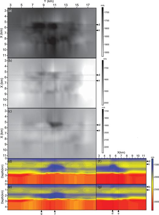
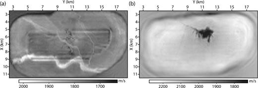
Slices of the initial model (vertical wave speed) built by reflection traveltime tomography (courtesy of BP) (a–c) Horizontal slices at (a) 175 m depth, (b) 500 m depth, (c) 1 km depth across the gas cloud. (d and e) Inline vertical slices (d) passing through the gas cloud (X = 5.6 km) and (e) near its periphery (X = 6.25 km). (f and g) Cross-line vertical slices at (f) Y = 11 km and (g) Y = 8.6 km.
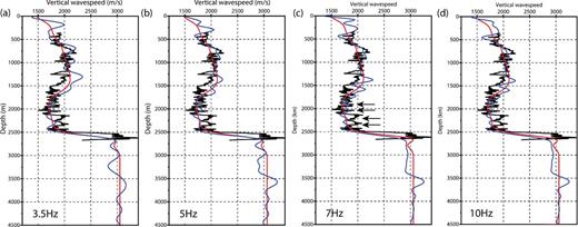
Comparison of velocity profiles extracted from the initial (red line) and FWI (blue line) models and sonic log (black line). (a) FWI model close of inversion of the initial frequency (3.5 Hz). (b) Same as (a) for the 5 Hz frequency. (c) Same as (a) for the 7 Hz frequency. (d) Same as (a) for the 10 Hz frequency. The arrows in (c) point on different layers that are discussed in the text.
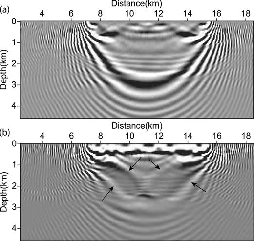
7 Hz monochromatic sensitivity kernel (or wave path) computed (b) in the initial model (Fig. 4) and (a) in the initial model after smoothing with a 3-D Gaussian smoother with a 500 m correlation length in the three Cartesian directions. In (b), the arrows point on the transmission paths followed by the reflected wave from the reservoir reflector (see text for complementary details).
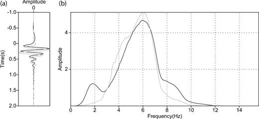
Synthetic seismograms computed in this initial model are shown in Fig. 8 for the receivers r1 and r2, together with the source wavelet that was used to generate these seismograms. These synthetic seismograms were computed with a classical |${\mathcal {O}}(\Delta t^2, \Delta x^8)$| staggered-grid finite-difference time-domain method for VTI acoustic media. Note that attenuation is not taken into account in these time-domain simulations. We first compute seismograms using a Dirac source wavelet. Then, we refine the source wavelet by linear inversion that aims to match the recorded seismograms and the modelled ones, assuming the subsurface model known (Pratt 1999). Before estimation of the source wavelet, we apply to the recorded data a Butterworth filter within the 3–7 Hz pass-band. The synthetic seismograms computed in the starting model mainly show the diving waves as well as the post-critical reflection from the top of the reservoir. The traveltimes of the diving waves are pretty well matched suggesting that the long wavelengths of the vertical wave speed and Thomsen parameter ϵ are fairly accurate. Of note, the bright critical reflection from the reservoir level is well reproduced from a qualitative viewpoint by the initial model (Fig. 8a, black dash arrow). Vertical velocity gradient in the initial model generates high amplitudes in the early arrivals at around 4.5 km of offset in Figs 8(a) and (b), dash red arrows. These high amplitudes reasonably mimic those of the critical reflection (and/or the caustic) from the shallow subsurface for the receiver r2 (Fig. 3b, dash red arrow). In contrast, these high amplitudes are clearly modelled at too large offset for receiver r1, suggesting that the shallow structure in the gas cloud area requires refinement (Fig. 3a, dash red arrow).
Synthetic seismograms computed in the initial models (Fig. 4) for the receivers r1 (a) and r2 (b) and for the inline shot profile passing through the receiver position (right panels). These seismograms can be compared with the corresponding real data shown in the left panels. The inset shows the source signature estimated by matching impulsional synthetic seismograms and recorded seismograms in the frequency domain.
A density model was built from the initial vertical velocity model following a polynomial form of the Gardner law given by |$\rho = -0.0261 \, V_0^2 + 0.373 \,V_0 + 1.458$| (Castagna et al.1993) and was kept fixed over iterations. A homogeneous model of the quality factor was used below the sea bottom with a value of QP = 200. This average value is inspired from the one estimated by Prieux et al. (2011) by matching the amplitude-versus-offset trend of the early arrivals.
3.1.4 Experimental setup
We sequentially perform 11 mono-frequency inversions using the final model of one inversion as the initial model of the next inversion (3.5 Hz, 4 Hz, 4.5 Hz, 5 Hz, 5.2 Hz, 5.8 Hz, 6.4 Hz, 7 Hz, 8 Hz, 9 Hz, 10 Hz). The starting frequency of 3.5 Hz was chosen according to the previous study of Sirgue et al. (2010). The grid intervals for seismic modelling are 70 m, 50 m, 35 m for the frequency bands [3.5 Hz; 5 Hz], [5.2 Hz; 7 Hz], [8 Hz; 10 Hz], respectively. These grid intervals roughly satisfy the sampling criterion of four gridpoints per minimum wavelength, which is suitable for FWI, the resolution of which is half the propagated wavelength. Note that the 70 m and 35 m grid intervals allow to match quite accurately the sea bottom at 70 m depth unlike the 50 m grid interval. This prompts us to set the first frequency processed on the 50 m grid (5.2 Hz) close to the last frequency processed on the 70 m grid (5 Hz). The sources and the receivers are positioned in the coarse finite-difference grids with the windowed sinc parametrization of Hicks (2002). No regularization and no data weighting were used. The source signature estimation, which consists of solving a linear inverse problem (Pratt 1999), is alternated with the subsurface update during each non-linear iteration. One source signature is averaged over the number of sources that are simultaneously processed by the direct solver during the substitution step (80, 30 and 10 on the 70 m, 50 m and 35 m grids, respectively). All the 49 954 shots and all of the 2302 hydrophones are involved in the inversion during each FWI iteration. Seismic modelling is performed with a free surface on top of the finite-difference grid during inversion. Therefore, free surface multiples and ghosts were left in the data and accounted for during FWI. We did not use an automatic stopping criterion of iterations. We empirically stopped the iterations when the update of the subsurface models became negligible. The significance of the model update from one iteration to the next may be measured by the following metric: |$u_m = \frac{|{{\bf m}}_{k+1} - {{\bf m}}_{k}|}{|{{\bf m}}_{k}|}$|, where k stands for the iteration number. We used um of the order of 10−2 for the frequencies between 3.5 Hz and 7 Hz and 10−3 for the frequencies between 8 Hz and 10 Hz. A more careful design of an automatic stopping criterion of iteration will deserve future work to avoid unnecessary iterations. We only update the vertical wavefield during inversion, while the density, the quality factor and the Thomsen's parameters are kept to their initial values.
Monochromatic receiver gathers at frequencies 3.5 Hz, 5 Hz, 7 Hz and 10 Hz are shown in Fig. 9 for the receiver r1. Although the footprint of noise is significant in Fig. 9(a), useful signal can be clearly observed on this gather. Note that most of the gathers have a much poorer signal-to-noise ratio at 3.5 Hz than the one shown in Fig. 9(a). Comparison between the recorded 7 Hz monochromatic receiver gather (receivers r1 and r2) and the corresponding synthetic receiver gather computed in the initial model highlights how the incomplete modelling of the reflection wavefields shown in Fig. 8 translates into phase and amplitude mismatches in the frequency domain (Fig. 10). As for time-domain modelling, we first perform frequency-domain modelling with a Dirac source signature before updating the source signature by minimization of the misfit between the monochromatic recorded data and the monochromatic Green's functions, assuming the subsurface medium known. Multiplication of the refined source signature with the monochromatic Green's function gives the monochromatic wavefield ready for comparison with recorded data. The same source estimation procedure is used to perform modelling in the FWI models (section Quality control of FWI results by seismic modelling).
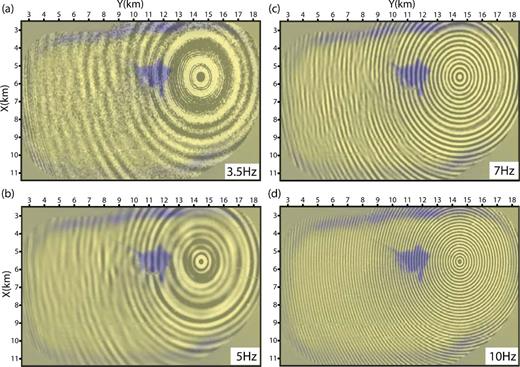
Monochromatic common-receiver gather for receiver r1. (a) 3.5 Hz. (b) 5 Hz. (c) 7 Hz. (d) 10 Hz. The frequencies 3.5 Hz and 10 Hz are the starting and the final frequencies that were used for FWI. The frequencies 5 Hz and 7 Hz are the final frequencies that were used on the 70 m and 50 m grids, respectively. The horizontal slice of the gas cloud is superimposed to gain some qualitative insights on the influence of the gas cloud on the seismic wavefield.
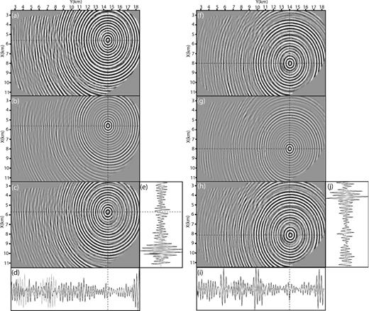
(a–e) Mismatch between the recorded (a) 7 Hz monochromatic receiver gather (receiver r1) and the corresponding synthetic (b) receiver gather computed in the initial model (Fig. 4). The real part is shown. (c) Difference between (a) and (b). The amplitudes are shown with the same amplitude scale in (a–c). (d and e) Direct comparison between recorded (black) and modelled (grey) gather in the inline (d) and cross-line (e) directions across the receiver position. Note the strong amplitude mismatch. Amplitudes are scaled with a linear gain with offset to correct for geometrical spreading. (f–j) Same as (a–e) for receiver r2.
We directly applied FWI to the data provided by BP without additional preprocessing. These data were subsampled with a sampling rate of 32 ms and bandpass filtered accordingly. A mute above the first arrival was also applied. Since the discrete frequencies were inverted sequentially (i.e. independently), the relative amplitude of these frequencies (i.e. the amplitude spectrum of the data) does not play any role in terms of data weighting during our FWI application.
3.2 FWI results
In Fig. 11, we extract horizontal and vertical slices of the final 10 Hz FWI model at the same positions as those of the initial model shown in Fig. 4. For plotting purpose, we resample the final velocity model on a fine Cartesian grid with a grid interval of 12.5 m.
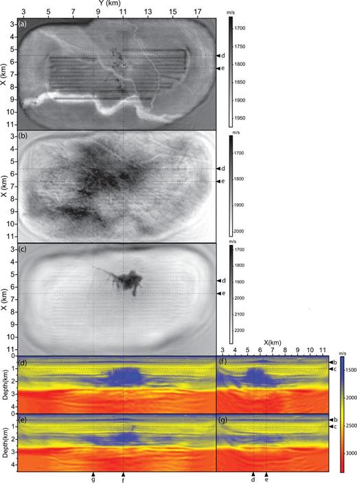
Slices of the 10 Hz FWI model, that can be compared with those of the initial model (Fig. 4). (a–c) Horizontal slices at (a) 175 m depth, (b) 500 m depth, (c) 1 km depth across the gas cloud. (d and e) Inline vertical slices (d) passing through the gas cloud (X = 5.6 km) and (e) near its periphery (X = 6.25 km). (f and g) Cross-line vertical slices at (f) Y = 11 km and (g) Y = 8.6 km. See text for interpretation.
The horizontal slice at 175 m depth shows high-velocity glacial sand channel deposits, which are similar to the ones shown in Sirgue et al. (2010, their fig. 9b) and Barkved et al. (2010) as well as low-velocity anomalies, which might be the subsurface expression of gas pockmarks and chimneys (Fig. 11a). These channels are completely absent from the initial model (Fig. 4a). The footprint of the receiver cables is visible although it becomes less awkward over the FWI iterations as the stack of several frequency contributions makes this footprint more spatially focused. As was mentioned in Sirgue et al. (2010) and Warner et al. (2013b), the image of the channels extends far beyond the area covered by the cables, suggesting that these channels are built from waves that mainly propagate subhorizontally (refracted waves or lateral reflections). Note also that at these depths anisotropy is negligible (Fig. 5a). Therefore, we do not expect any difference in the positioning in depth of these channels relative to the results of Sirgue et al. (2010).
The horizontal slice at 500 m depth shows several linear features that were interpreted by Sirgue et al. (2010, their fig. 8b) as scrapes in the palaeo-seafloor left by drifting icebergs (Fig. 11b). These short-scale features are again absent from the initial model (Fig. 4b). This horizontal slice also maps a widespread low-velocity zone.
The horizontal slice at 1 km depth (Fig. 11c) shows how the image of the gas cloud has been significantly refined. A set of low-velocity small-scale structures, probably some fractures, radiate out from the gas cloud [see Sirgue et al. (2010, their fig. 4c) for a comparison].
We tentatively reduce the acquisition footprint in the horizontal slices at 175 m and 1 km depth in the wavelet domain (Fig. 12). We transform the slice in the wavelet domain using Daubechies wavelets with 20 vanishing moments and cancel out the shortest horizontal scales before transforming back the slice in the spatial domain.
The inline vertical section in Fig. 11(d) shows a shallow low-velocity reflector at 0.5 km depth above a positive velocity gradient (see also Fig. 6d), which can be correlated with the shallow reflection highlighted in Fig. 3, red dash arrows. The extension of this low-velocity zone in the horizontal plane is shown in Fig. 11(b). The geometry of the gas cloud in the vertical plane has been nicely refined after FWI and compares well with the image shown in Sirgue et al. (2010, their fig. 2b). The base cretaceous reflector at 3.5–3.7 km depth, highlighted in Fig. 2(b), is also fairly well imaged, as well as in the cross-line direction (Figs 11f and g). The positive velocity contrast associated with this reflector can be assessed along the vertical profile extracted at the well log position (Fig. 6, 3.5 km depth). At these depths, FWI behaves as a least-squares migration as deep targets are mainly illuminated by reflections. Another inline vertical section of the final FWI model at X = 6.25 km (Fig. 11e) shows the footprint in a vertical plane of a north-south fracture previously identified in Fig. 11(c) at Y = 11.5 km [see also Sirgue et al. (2009, their fig. 3b) for a comparison].
All these features are synthesized in Fig. 13, which shows three expositions of the interior of the FWI V0 volume. The first is focused on a vertical section across the gas cloud down to the reservoir and the base cretaceous reflector. The second shows the horizontal slice across the gas cloud at 1 km depth together with a vertical section on the periphery of the gas cloud to emphasize the 3-D geometry of several subvertical fractures radiating out from the gas cloud. The third shows the interior of the volume outside of the gas cloud area. On the three panels of Fig. 13, quite focused migrated-like images of deep reflectors show how FWI allowed for imaging below the reservoir level although the presence of gas in the overburden and how the geometry of these reflectors evolves as we move away from the zone of influence of the gas.
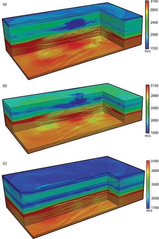
3-D perspectives of the final FWI model. (a) Vertical section across the gas cloud, the reservoir and the base cretaceous reflector. (b) Depth slice of the gas cloud (1 km depth) and vertical section at the periphery of the gas cloud, that highlight the geometry of several subvertical fractures. (c) Vertical sections off the gas cloud. Note how the geometry of the reflectors below the reservoir level evolves from (a) to (c).
The multiscale nature of the frequency-domain FWI is illustrated in Fig. 14, which shows the horizontal section of the gas cloud at 1 km depth and one inline and cross-line vertical sections of the FWI models obtained closed of the inversion of the 3.5 Hz, 5 Hz, 7 Hz and 10 Hz frequencies. The inline and cross-line sections are those shown in Figs 11(e) and (g). The resolution improvement from the 3.5 Hz to the 7 Hz frequency is obvious both in the horizontal and vertical planes. The structures become sharper and better focused as additional frequencies contribute to broaden the wavenumber spectrum of the subsurface model. More disappointingly, the improvements of the subsurface model in the 8–10 Hz frequency band are more subtle. Frequencies between 8 Hz and 10 Hz mainly contribute to better resolve shallow structures above 500 m depth and decrease the acquisition footprint above the low-velocity zone (compare panels c and d of Fig. 14). This latter point is clearer in the cross-line directions due to the coarser sampling of the receiver domain. The limited contribution of the 8–10 Hz band might result from several factors: an inappropriate data weighting putting too much weight on the short-offset/early-arriving phases keeping in mind that long-offset wavefield amplitudes tend to attenuate faster as frequency increases, inaccurate amplitude processing due to the fact that only V0 is updated during FWI and inaccurate physics for seismic modelling.
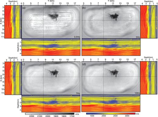
FWI models obtained close of the inversion of the 3.5 Hz frequency (a), 5 Hz frequency, 7 Hz frequency (c) and 10 Hz frequency (d). See text for details.
Comparison between the sonic log and the corresponding vertical profile of the 10 Hz FWI model shows that the sharp reflector at 0.5 km depth is well delineated by a low-velocity anomaly (Fig. 6d). The velocity gradient between 0.5 km and 0.75 km depth is also reasonably well matched. The velocities of the FWI velocity model are higher than those of the sonic logs between 1.25 km depth and 1.7 km depth. Similar trend is shown in the FWI models of Prieux et al. (2011). This might be the footprint of cross-talk between V0 and the subsurface parameters that have been kept fixed during inversion. Update of density, attenuation and ϵ will be helpful to check whether they can correct for this mismatch. It is quite speculative to assess the quality of the velocity update in the low-velocity zone between 1.5 km and 2.5 km depth. FWI velocities seem to reproduce the alternation of high and low velocities shown in the sonic log between 1.7 km and 2.5 km depth (Fig. 6c, black arrows). However, the absolute velocities are not matched between 2.1 and 2.3 km depth. This might result from some missing intermediate vertical wavenumbers in the FWI model at these depths associated with the lack of diving wave illumination. As expected the reflector delineating the top of the reservoir was not moved at the well location where this reflector was quite sharp in the starting model. The base cretaceous reflector is successfully identified by a sharp positive velocity contrast at 3.5 km depth, this depth being consistent with the image of this reflector in the migrated image shown in Fig. 2(b). Fig. 6 also shows the FWI logs for the 3.5 Hz, 5 Hz and 7 Hz frequencies to complement the multiscale analysis illustrated in Fig. 14. Comparison between the 7 Hz and 10 Hz FWI logs shows how the shallow sedimentary layer between the sea bottom and 0.5 km depth was sharpened after the 10 Hz inversion. In contrast, some deeper velocity contrasts seem to have been subdued after the 10 Hz inversion. This might result because the quality factor was kept fixed to a constant value during FWI (QP = 200) and the footprint of attenuation in the data might increase with frequency. Underestimated velocity contrasts after the 10 Hz inversion might highlight cross-talks between velocity and QP factor that compensate for underestimated attenuation (overestimated QP) in the background model.
3.3 Quality control of FWI results by seismic modelling and source wavelet estimation
In the following, we control the quality of the FWI models by seismic modelling and source wavelet estimation.
3.3.1 Misfit reduction
The misfit function reduction and the number of FWI iterations performed during each mono-frequency inversion are outlined in Table 1. The misfit function reduction ranges between 4.7 per cent at 3.5 Hz and 73.4 per cent at 8 Hz. The number of FWI iterations ranges between 4 at 9 Hz and 24 at 7 Hz. The limited misfit function reduction at 3.5 Hz results from the poor signal-to-noise ratio at this frequency. Although the velocity model was not very significantly updated between the 7 Hz and the 8 Hz inversions, the highest misfit function reduction was achieved at 8 Hz. This might result from the finite-difference grid refinement between the 7 Hz and 8 Hz inversion, which probably modified the velocity structure of the sea bottom and hence the match of the short-offset high-amplitude arrivals. This issue probably deserves more detailed and careful investigations in the future.
Misfit function reduction for each successive mono-frequency inversion. f(Hz): frequency. |$\#it$|: number of FWI iterations. mfr(per cent) = 100 × (Cf − C0)/C0: misfit function reduction in percentage of the initial value C0 of the misfit function. The limited misfit function reduction at 3.5 Hz results from the poor signal-to-noise ratio at this frequency.
| f (Hz) | 3.5 | 4 | 4.5 | 5 | 5.2 | 5.8 | 6.4 | 7 | 8 | 9 | 10 |
| |$\#it$| | 19 | 14 | 12 | 14 | 17 | 12 | 17 | 24 | 11 | 4 | 17 |
| mfr (per cent) | 4.7 | 25.7 | 42.7 | 57 | 42.6 | 39.6 | 33.1 | 27.2 | 73.4 | 12.7 | 41.8 |
| f (Hz) | 3.5 | 4 | 4.5 | 5 | 5.2 | 5.8 | 6.4 | 7 | 8 | 9 | 10 |
| |$\#it$| | 19 | 14 | 12 | 14 | 17 | 12 | 17 | 24 | 11 | 4 | 17 |
| mfr (per cent) | 4.7 | 25.7 | 42.7 | 57 | 42.6 | 39.6 | 33.1 | 27.2 | 73.4 | 12.7 | 41.8 |
3.3.2 Frequency-domain data fit
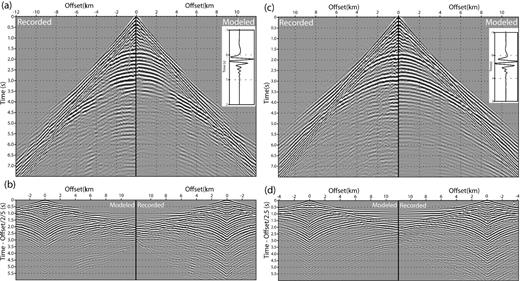
For sake of figure readability, we compare recorded and modelled monochromatic receiver gathers at the 7 Hz frequency rather than at the 10 Hz frequency (Fig. 15). Few insights on the match between recorded and modelled data at other frequencies are discussed later in this study. Modelling is performed in the FWI model obtained close of the 7 Hz frequency inversion. Overall, we show an excellent match between the recorded and modelled data. Compared to the frequency-domain modelling performed in the initial model (Fig. 10), the data fit has been dramatically improved over the full range of offsets as the inversion injects in the subsurface models short-scale variations, which allow to explain both the pre-critical and post-critical reflections highlighted in Fig. 3. It is worth noting some overestimated modelled amplitudes at large offsets in Fig. 15(d), ellipse (receiver r1) that are not shown in Fig. 15(i) (receiver r2). This again might highlight the footprint of underestimated attenuation effects in the modelled amplitudes. It is likely that the attenuation footprint is higher in the wavefields that propagated across the gas cloud as it is the case of the wavefields recorded by receiver r1 compared to r2.
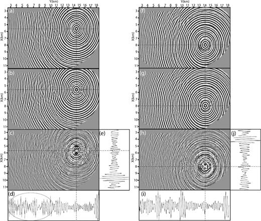
(a–e) Comparison between the recorded 7 Hz monochromatic receiver gather (a) and the corresponding synthetic receiver gather computed in the 7 Hz FWI model (b) for the receiver r1. (c) Difference between (a) and (b). (d and e) Direct comparisons between the recorded (black line) and modelled data (grey line) along inline (d) and cross-line (e) profiles passing through the receiver position. Amplitudes are scaled with a linear gain with offset to correct for geometrical spreading. The ellipse highlights where modelled amplitudes tend to be overestimated. (f–j) Same as (a–e) for receiver r2. Note that overestimation of modelled amplitudes is less apparent. See text for interpretation. The improvement of the data fit achieved after FWI can be assessed by comparison with Fig. 10.
In efficient frequency-domain FWI, discrete frequencies are inverted sequentially from the low frequencies to the higher ones. When the inversion inverts a new frequency component, the former lower frequencies are not involved anymore in the inversion for computational cost reasons. Although the theoretical justification of this frequency hopping approach is reviewed in the Introduction, we cannot formally guarantee that the FWI model updated after one frequency inversion still allows one to match the data at lower frequencies. For a qualitative assessment of the frequency hopping strategy, we compare the data fit achieved at a given frequency when the modelling is performed in the final 10 Hz FWI model and in the FWI model inferred from the inversion of the frequency in question. This comparison is shown for the 3.5 Hz, 5 Hz, 7 Hz frequencies in Figs 16 and 17(a). For sake of completeness, we also show in Fig. 17(b) the excellent 10 Hz data fit that is achieved when modelling is performed in the final 10 Hz FWI model. Results clearly show that the 3.5 Hz, 5 Hz and 7 Hz data fits are degraded when seismic modelling is performed in the final 10 Hz FWI model rather than in the FWI models inferred from the inversion of the frequency in question. This degradation logically decreases from low frequencies to higher ones, namely, as the frequency becomes closer to 10 Hz. Only the amplitude fit is significantly degraded compared to the phase which is still quite accurately matched. Be that as it may, these results suggest that it may be worth performing several V or W cycles of FWI by going forth and back over frequencies and finite-difference grids following some paths that need to be defined. This investigation, which mimics a multigrid procedure, is left for future work. Another possible interpretation of this degraded fit might be related to attenuation-related dispersion.
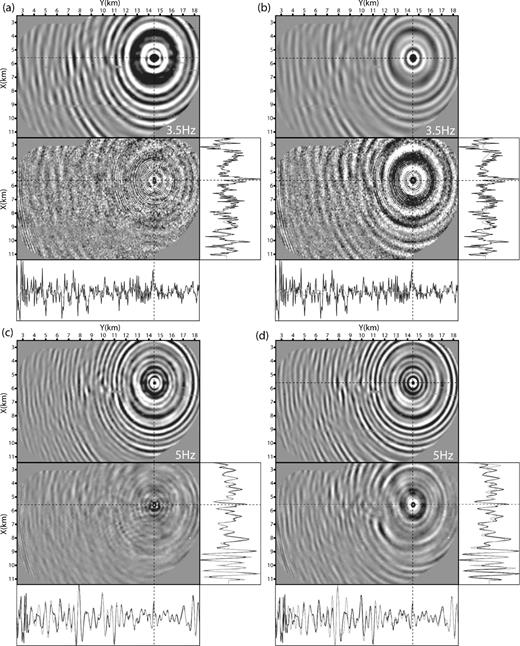
(a and b) Frequency-domain modelling at 3.5 Hz for receiver r1. (a) Modelling is performed in the FWI model obtained close of the 3.5 Hz inversion. (b) Modelling is performed in the final 10 Hz FWI model. The top panel shows the modelled gather. The bottom panel shows the difference between the recorded gather (Fig. 9a) and the modelled one (a). Direct comparison between recorded and modelled wavefields along two profiles running across the receiver position are also shown following the same representation as in Fig. 15(a–e). (c and d) Same as (a and b) for the 5 Hz frequency.
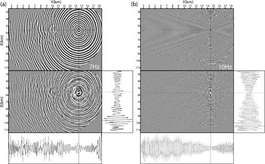
(a) Frequency-domain modelling at 7 Hz for receiver r1. Modelling is performed in the final 10 Hz FWI model. The top panel shows the modelled gather. The bottom panel shows the difference between the recorded gather (Fig. 9c) and the modelled one (a). Following the same assessment procedure as in Fig. 16, the data fit can be compared with the one that is achieved when modelling is performed in the FWI model obtained close of the 7 Hz inversion (Fig. 15). (b) Frequency-domain modelling at 10 Hz for receiver r1. Modelling is performed in the final 10 Hz FWI model. The 10 Hz recorded receiver gather is shown in Fig. 9(d).
The fact that FWI allows us to fit the data in the frequency domain does not guarantee that the inversion was not hampered by cycle skipping. To assess whether cycle skipping generate artefacts in the FWI models, we now analyse the data fit in the time domain (for all the frequencies in the 3–7 Hz frequency band).
3.3.3 Time-domain data fit
We compute time-domain VTI acoustic seismograms in the 10 Hz FWI model for the receivers r1 and r2 with the approach described in the section Starting FWI subsurface model: first, synthetic seismograms are computed with a Dirac source wavelet; second, the source wavelet is refined by matching the recorded seismograms with the modelled ones, after Butterworth filtering of the recorded data in the 3–7 Hz frequency band. We recall that attenuation is not taken into account in these modelling. Results of this modelling are shown in Fig. 18 for receivers r1 and r2.
Time-domain modelling for receivers r1 and r2 and inline shot profiles passing through the receiver positions. (a and b) Receiver r1. Modelling is performed in the final 10 Hz FWI model. (a) (left-hand side) Recorded data. (Right-hand side) Mirrored modelled synthetics. (b) (Left-hand side) Mirrored modelled synthetics. (Right-hand side) Recorded data. In (b), the seismograms are plotted with a linear moveout (equal to offset divided by a reduction velocity of 2.5 km s−1) to favour the interpretation of diving waves and super-critical reflections. The estimated source wavelet is shown in the insert. (c and d) Same as (a and b) for receiver r2.
From a qualitative viewpoint, the modelled seismograms reproduce the key features of the recorded data that were discussed in section Seismic acquisition and data set at both pre-critical and post-critical incidences (reflections from the shallow reflector, from the top of the gas, from the reservoir). Comparison between the synthetic seismograms computed in the starting model (Fig. 8) and in the final FWI model (Fig. 18) highlights the significant amount of data information that were added to the modelled seismograms after FWI.
Validation of FWI model reflectors and phase interpretation in the receiver gathers can be further refined by checking the local setting between the FWI model after depth-to-time conversion and zero-offset reflections in the receiver gathers (Fig. 19). Figs 19(a) and (d) show two inline vertical section of the final 10 Hz FWI model along cables 13 (i.e. across the gas cloud) and 21 (i.e. across the sonic log) on which we superimpose their vertical derivative to emphasize the velocity contrasts. Figs 19(b) and (e) show the corresponding sections after depth-to-time conversion. We superimpose on the two-way time sections a common receiver gather in Figs 19(c) and (f) to check the setting between the FWI reflectors and the zero-offset reflections. Figs 19(c) and (f) confirm that the 3 s two-way traveltime zero-offset reflection corresponds to the reflection from the reservoir level. Fig. 19(c) shows that the intra-gas reflector below the gas cloud at around 1.7 km depth (Fig. 19a) matches quite well a major reflection in the data at 2.2 s two-way traveltime. Fig. 19(f) confirms that the 1.8 s zero-offset reflection corresponds to the reflection from the top of the low-velocity zone. The setting between the base cretaceous reflector and low-amplitude reflections is also illustrated in Figs 19(c) and (f).
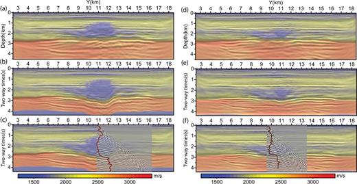
Reflector identification in the 10 Hz FWI model. (a, d) FWI model superimposed on its vertical derivative along cables 13 (a) and 21 (d). (b and e) Same as (a and d) after depth to two-way traveltime conversion. (c and f) Same as (b and e) with superimposed common receiver gather and vertical profile (black curve) of the FWI model. Note the correlation between the zero-offset reflections and the reflectors of the FWI model.
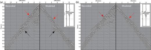
A close look of Fig. 18 suggests that the recorded and modelled diving waves at long offsets as well as the reflection from the top of the reservoir are not rigorously in phase. We quantify more precisely this mismatch in Fig. 20 in which we superimpose in transparency the modelled data plotted with a variable area wiggle display on the recorded data plotted with a blue-white-red colour scale. The two sets of seismograms match each other if the black area of the modelled seismograms hides the blue part of the recorded wavefield. We do not apply any delay to the modelled seismograms in Fig. 20(a), while we delay the modelled seismograms by 40 ms in Fig. 20(b). We show that the modelled and recorded seismograms are in phase in Fig. 20(a) for the diving waves recorded for a maximum offset of around 4 km and for the reflections from the shallow reflector and from the top of the low-velocity zone. Then, we start noticing some phase mismatch. A delay of 40 ms makes the two wavefields to be in phase for the later arriving phases, namely, the post-critical reflection from the top of gas and the reflection from the top of the reservoir.
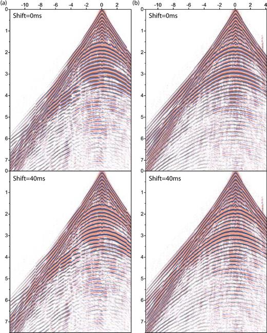
Direct comparison between recorded and modelled seismograms. The recorded seismograms are plotted with a blue-white-red colour scale, while the modelled seismograms plotted with a variable-area wiggle display are superimposed with 40 per cent of opacity. The two sets of seismograms are in phase if the black variable area of the modelled seismograms hides the blue part of the recorded seismograms. Top panel: No time-shift is applied to the modelled seismograms. Bottom panel: A 40 ms traveltime delay is applied to the modelled seismograms. (a) Common-receiver gather r1. (b) Common-receiver gather r2.
It is difficult to conclude whether the advance of the modelled arrivals relative to the recorded ones results from the difference between the modelling engines that were used to perform frequency-domain FWI and time-domain modelling, an accumulation of inaccuracies with propagating time, an increasing kinematic inconsistency with scattering angle keeping in mind that the anisotropic parameter ϵ is kept fixed during the inversion or inaccurate modelling of elastic and attenuation effects. This issue is discussed in more details in the final discussion section. A time-shift of 40 ms corresponds to a period of the 25 Hz frequency, which is significantly higher than the maximum frequency involved in the inversion (10 Hz). We conclude that cycle skipping didn't hamper significantly the FWI results.
3.3.4 Source wavelet estimation
The seismic wavefield depends both on the subsurface properties and the temporal source signature if we assume that the radiation pattern and the position of the sources in the subsurface are known. In controlled-source seismology, it is reasonable to assume that the source signature does not vary from one shot to the next. Therefore, the source signature estimation can be used as a quality control of the FWI models: a temporal source signature is estimated for each source gather from the FWI model with the procedure described in section Starting FWI subsurface model. The focusing and the repeatability of the signatures from one shot to the next provides some insight on the quality of the subsurface model. Some differential semblance optimization applied on the source wavelet gather can also be used to update the subsurface model as proposed by Pratt & Symes (2002) and Gao et al. (2014).
We apply this quality control to 175 common-receiver gathers evenly distributed over the cable layout (Fig. 21). We estimate the source wavelets from the initial model (Figs 21a–d) and the final 10 Hz FWI model (Figs 21e–h). We first show the estimated wavelets when no gain with offset is applied to the data (Figs 21a and e). In this case, the wavelet estimation is dominated by the high-amplitude, short-offset, early arrivals and hence is less sensitive to the accuracy of the subsurface model. The wavelets estimated in the initial and final FWI models show a good repeatability, hence supporting the moderate sensitivity of the source wavelet estimation to the accuracy of the subsurface model in this setting. We note however that the absolute amplitudes of the wavelets estimated in the initial model are around two times smaller than those estimated in the FWI model. This is a first indicator of the relevance of the FWI model. The same wavelet representation after normalization of each wavelet by its maximum amplitude confirms that the repeatability of the wavelets is similar when they are estimated from the initial and final FWI models (Figs 21b and f).
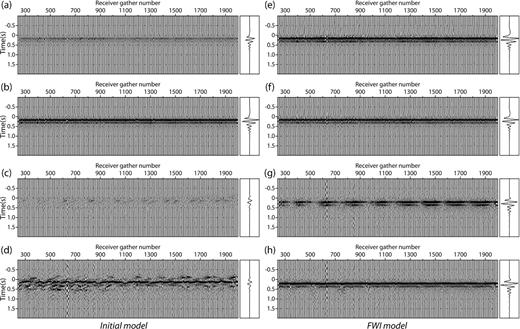
Quality control of FWI model by source wavelet estimation. (a-d) Source wavelets estimated from the initial model. (e-h) Source wavelets estimated from the final 10 Hz FWI model. (a, e) Source wavelets are estimated from unweighted data and are plotted without normalization. (b, f) Same as (a, e) except that each wavelet is normalized by its maximum amplitude. (c, g) Source wavelets are estimated from data to which a linear gain with offset was applied and are plotted without normalization. (d, h) Same as (c, g) except that each wavelet is normalized by its maximum amplitude. The wavelet on the right of each wavelet gather is the average wavelet. The wavelets are plotted with the same amplitude scale on each row (a, e), (b, f), (c, g), (d, h) for a fair comparison between the wavelets estimated from the initial and final FWI models. See text for more details.
In a second step, we apply a linear gain with offset to the data in order to increase the sensitivity of the source wavelet estimation to the accuracy of the subsurface model. The effect of the gain with offset on the data amplitudes is shown in Figs 15(d), (e), (i) and (j). The results of the source wavelet estimation are shown in Figs 21(c, g) and 21(d, h) without and with amplitude normalization of the wavelets, respectively. We show now how both the repeatability and the absolute amplitude of the wavelets are impacted when the initial subsurface model does not allow to predict the full wavefield (Fig. 21c). In contrast, the repeatability in terms of shape and timing remains good when the wavelet estimation is performed with the final FWI model, although periodic amplitude variations are shown in the wavelet gather (Fig. 21g). These periodic variations show higher-amplitude wavelets when the corresponding receivers are located nearby the centre of the cable and lower-amplitude wavelets when the corresponding receivers are located nearby the ends of the cable. This pattern illustrates on the one hand the higher sensitivity of the wavelet estimation to long-offset arrivals when a linear gain with offset is applied to the data and on the other hand the higher sensitivity of long-offset data to the inaccuracies of the FWI model. Although we point out these amplitude inaccuracies, the repeatability of the source wavelets remains far better when it is performed in the final FWI model rather than in the initial model. A clearer picture of the repeatability of the source wavelets is shown in Figs 21(d) and (h) where each wavelet is normalized by its maximum amplitude.
In Fig. 22(a), we show that the average wavelet estimated in the final FWI model from the unweighted (short-offset) data has a first break that is 40 ms earlier than the one of the average wavelet from the weighted (long-offset) data. This is consistent with the kinematic mismatch highlighted in Fig. 20 (note that source wavelets used to build seismograms shown in Figs 18 and 20 are estimated from unweighted data). The wavelet estimated from the long-offset data has also a slightly more limited high-frequency content according to the faster attenuation with offset of high frequencies (Fig. 22b).
3.4 Computational cost
To perform the FWI case study, we used the clusters Licallo and Froggy of high-performance computer centres SIGAMM (hosted at Observatory of Cote d'Azur, France) and CIMENT (Grenoble University, France). The statistics outlined in Table 2 were obtained on the Licallo cluster. The nodes of the Licallo cluster are composed of two 2.5 GHz Intel Xeon IvyBridge E5-2670v2 processors with 10 cores per processor. The shared memory per node is 64Gb. The connecting network is infiniband FDR at 56 Gb s−1.
Computational demand of frequency-domain FWI for the Valhall case study. f(Hz): frequency band processed for a given grid size. h: grid interval in meters. nu: number of millions of unknowns in the computational grid (including PMLs). |$\#n$|: number of computer nodes used during FWI. |$\#mpi$|: number of MPI processes. |$\#th$|: number of threads per MPI process. mlu(Gb): memory required by LU factorization in giga bytes. tlu(s): elapsed time for LU factorization in seconds. ts: elapsed time to compute one wavefield solution by forward/backward substitution. tms: elapsed time to compute all the incident and adjoint wavefield solutions (2 × 2302 wavefields) by forward/backward substitution. ng: number of computed gradients. tg(mn): elapsed time to compute one gradient in minutes.
| f (Hz) | h (m) | nu (106) | |$\#{n}$| | |$\#mpi$| | |$\#{th}$| | mlu (Gb) | tlu (s) | ts (s) | tms (s) | ng | tg (mn) |
|---|---|---|---|---|---|---|---|---|---|---|---|
| 3.5–5 | 70 | 2.94 | 12 | 24 | 9 | 84 | 86 | 0.16 | 736 | 76 | 35 |
| 5.2–7 / 6–7 | 50 | 7.17 | 16 | 32 | 9 | 288 | 378 | 0.37 | 1703 | 118/69 | 60 |
| 8–10 | 35 | 17.22 | 34 | 69 | 9 | 1645 | 1260 | 1.1 | 5064 | 48 | 175 |
We used 12 nodes, 16 nodes and 34 nodes to perform FWI on the 70 m, 50 m and 35 m grids, respectively. We launch two MPI processes per node (i.e. one MPI process per processor) and use 10 threads per MPI process such that the number of MPI processes times the number of threads equal to the number of cores on the node. We limit the number of MPI process per node to mitigate the volume of communication and the memory overheads during the multifrontal factorization and we take advantage of multithreaded distribution of the BLAS3 to perform efficiently the dense linear algebra tasks performed by MUMPS during the factorization and substitution steps. During the substitution step, we jointly process 80, 30 and 10 right-hand sides (either incident sources or residual sources) in one go on the 70 m, 50 m and 35 m grids, respectively. All the computations were performed in single precision. All the computations were performed in core memory without access to hard disk except for reading the data and writing the FWI subsurface models and the wavefield solutions at receiver positions (this last writing is optional but the cost provided in Table 1 include this task).
We draw the following conclusions from the statistics outline in Table 2:
Although the LU factorization and the multi-right-hand sides substitution have the same time complexity (|${\mathcal {O}}(n^6)$|), the cost of the LU factorization is relatively small compared to the time dedicated to the substitution steps: the cost LU factorization is 11.5 per cent, 22 per cent and 25 per cent of the one of the solution steps on the 70 m, 50 m and 35 m grids, respectively. This results from the large number of right-hand sides to be processed for this case study (4604).
The elapsed time to compute one wavefield solution, once the LU factorization was performed, is 0.16 s, 0.37 s, 1.1 s on the 70 m, 50 m, 35 m grids, respectively. This highlights the benefit of frequency-domain modelling based on sparse direct solver to process a large number of seismic sources very efficiently.
The memory required by the LU factorization is tractable at these frequencies: 84 Gb, 288 Gb, 1.645 Tb on the 70 m, 50 m and 35 m grids, respectively. The memory demand is sufficiently low to allows us to perform all the computations in core memory.
The elapsed time to compute one gradient is around 35 mn, 60 mn, 175 mn on the 70 m, 50 m, 35 m grids, respectively. The tasks performed by MUMPS (LU factorization and substitution steps) roughly represent one half of the elapsed time required to compute one gradient. Presently, most of the computations that are not related to MUMPS (building of right-hand sides, explicit computation of pv wavefield, extraction of wavefield solutions at receiver positions, source signature estimation, computation of data residuals and misfit function, building of the radiation pattern matrices and correlation between incident and adjoint wavefields) are parallelized with MPI through a source distribution over the MPI processes. Only the reading of the data, the writing of the FWI models and the line search are sequential. Combining this MPI parallelism with Open Multi-processing (OpenMP) parallelism should help to further reduce significantly the cost of these tasks.
To obtain the results shown in this paper, we computed 76, 118 and 48 gradients on the 70 m, 50 m, 35 m grids, respectively. The elapsed times to generate the FWI models after the 7 Hz inversion and the 10 Hz inversion are roughly 6.8 d and 12.6 d, respectively. If two frequencies (6 and 7 Hz) would have been processed on the 50 m grid instead of four (5.2 Hz, 5.8 Hz, 6.4 Hz and 7 Hz) as in Sirgue et al. (2010), the elapsed time to generate the FWI models after the 7 Hz inversion would have been of the order of 4.7 d. We checked that with this coarse frequency sampling, quite reliable results (not shown here) are also obtained. These numbers are provided for reference only since they strongly depend on the number of non-linear FWI iterations. As the inversion approaches the minimum of the objective function, the line search often requires several gradient computations before finding a step length. A more aggressive stopping criterion of iterations than the one used in this study would have allowed us to reduce the number of gradient computations without hampering significantly the quality of the FWI models.
4 DISCUSSION
We have presented the first application on real ocean-bottom seismic data of 3-D efficient frequency-domain FWI based on sparse direct solver when attenuation and VTI anisotropy are taken into account in the modelling. The quality of the subsurface velocity models down to the reservoir is close to the one obtained during a previous study (Sirgue et al.2010) for which seismic modelling is performed in the time domain while the inversion is performed in the frequency domain using an isotropic approximation. At 175 m depth, we successfully imaged with a high resolution a glacial channel system as well as several short-scale low-velocity anomalies. At 500 m depth, we image the footprint of drifting icebergs on the palaeo seafloor as well as a wide-spread low-velocity zone, whose footprint is well identified in vertical sections by a sharp low-velocity reflector. Deeper, a depth slice at 1 km depth reveals the dramatic resolution improvement provided by FWI compared to reflection traveltime tomography to redefine the geometry of the gas cloud and identify several subtle features radiating out from it. Joint inspection of the horizontal slice across the gas cloud and vertical slices cross-cutting the gas cloud and its periphery confirms the resolution improvement of the gas-cloud image. Between 3 km and 3.7 km depth, FWI successfully imaged the base cretaceous reflector, previously identified on depth migrated images. At these depths, FWI mostly behaves as a least-squares reverse-time migration according to the available source–receiver offset range. It seems that we obtain a clearer migrated-like image of the base cretaceous reflector at 3.5–3.7 km depth than in Sirgue et al. (2010).
4.1 On the footprint of incomplete physics in mono-parameter FWI results
We control the quality of the FWI model by frequency-domain and time-domain modelling, source wavelet estimation and comparison with sonic log velocities. We review the three main observations that were inferred from this quality control before discussing their possible interpretation.
The data fit in the frequency domain is excellent in terms of phase and amplitude, although we notice some overestimation of the modelled amplitudes at long offsets, this overestimation being more pronounced for wavefields propagating across the gas cloud (Fig. 15). It is worth remembering that each frequency component was inverted separately from others, the dependency between each mono-frequency inversion being performed through the use of the final model of one frequency inversion as the starting model of the next frequency. Although each mono-chromatic data set involved in one mono-frequency inversion does not carry out the footprint of possible dispersion effects, any wave dispersion phenomena that would not be account for during seismic modelling will manifest during the inversion of one frequency component through some kinematic inconsistencies of the initial model inferred from the previous frequencies.
We show that late-arriving phases (diving waves and reflection from reservoir) computed by finite-difference time-domain modelling (without accounting for attenuation) arrive around 40 ms earlier than the corresponding recorded phases. This time-shift was confirmed by the source wavelet estimation: the source wavelet estimated from unweighted data (representative of short-offset early arrivals and used to perform the just mentioned time-domain simulation) has a first break located 40 ms earlier than the source wavelet estimated from weighted data (representative of long-offset arrivals).
Comparison between the sonic log and the 7 Hz and 10 Hz FWI models shows that velocity contrasts of the 10 Hz FWI model below 500 m depth seem to have been subdued compared to those shown in the 7 Hz FWI model (Fig. 6). Overall, the match between the sonic log and the FWI model is less than we expected owing the quality of the FWI model from a structural viewpoint.
Our favourite interpretation to explain these observations is related to underestimation of attenuation effects during seismic modelling. We used a constant QP of 200 to perform seismic modelling during FWI, while values as small as 40 are expected in unconsolidated sediments and gas zones (Prieux et al.2013a). We perform visco-acoustic finite-difference simulations in a two-layer model with an interface at 2.5 km depth using different values of QP in the upper layer (QP = 200 is used in the lower layer). Using the causal Kolsky-Futterman attenuation model with a reference frequency of 50 Hz allows us to generate a 40 ms time-shift between the reflection arrivals computed with QP = 200 and QP = 40 in the upper layer. The softening of the velocity contrasts in the FWI models as frequency increases might reveal some trade-offs between velocity contrasts and attenuation to match reflection amplitudes (Fig. 6). If some attenuation-related dispersion is present in the frequency band of interest, the imprint of the dispersion might explain some subtle mismatches in terms of depth positioning between sonic log and FWI velocities. This might also partly explain why the final 10 Hz FWI model does not allow to match the data at frequencies lower than 10 Hz as well as the FWI models generated by these frequencies (Fig. 16). If dispersion effects are generated by attenuation, mono-frequency inversions might be more suitable to reduce the footprint of this dispersion in the FWI results if attenuation is not involved in the inversion (this study). In contrast, simultaneous inversion of multiple frequencies or time-domain inversion might be more suitable to update attenuation by increasing the signature of the attenuation effects in the optimization problem and by reducing the trade-off between velocity and attenuation.
The density is another second-order parameter that was not involved in the inversion. It is well acknowledged that this parameter is strongly coupled with the velocity at short-scattering angles since the impedance, the product of velocity and density, controls the amplitude of short-spread reflections (e.g. Operto et al.2013). Some overestimation of the FWI velocities relative to the sonic log velocities might indicate some cross-talk effects between velocity and density during inversion as illustrated by Prieux et al. (2013a).
Indeed, acoustic modelling implies that the amplitude-versus-offset (AVO) behaviour of the P–P reflections does not account for elastic effects. These amplitude errors will generate reflected-wave residuals in the misfit function, that are amenable to long-wavelength velocity updates during their minimization even if the initial velocities allows for the accurate prediction of reflection traveltimes (Plessix et al.2014). This results because reflectors that are built in the velocity models over the FWI iterations by migration-like imaging behave as secondary sources in depth during inversion as long as the residuals generated by these reflectors have not been cancelled out. These secondary sources in depth are amenable to the update of the long-wavelengths of the subsurface through a tomographic-like reconstruction along the two paths of the reflected waves connecting the reflector to the source and the receiver (as those shown in Fig. 7b). We believe that these elastic effects are, however negligible in Valhall where the velocity contrasts are reasonably mild. To illustrate this statement, we compare seismograms for the hydrophone component computed in an acoustic and elastic Valhall models. The acoustic Valhall model corresponds to the final FWI model developed in this study. The elastic model shares V0, ρ, δ and ϵ with the acoustic model, while the vertical shear wave speed model was built from the FWI V0 model and the Poisson ratio computed in the elastic version of the reflection traveltime tomography model (courtesy of BP). The Thomsen parameter γ was chosen equal to ϵ. Comparison between acoustic and elastic seismograms shows no phase shift between the main P-wave arrivals as well as reasonably small amplitude differences (Fig. 23). Part of these amplitude differences might be absorbed by the source wavelet estimation during acoustic FWI. The relevance of the acoustic approximation for FWI in more complex and contrasted land environments is discussed in Plessix & Solano (2015) for comparison.
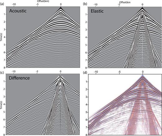
Hydrophone component. (a) Acoustic seismograms. (b) Elastic seismograms. (c) Difference between (a) and (b). (d) Direct comparison between (a) and (b). Elastic seismograms are plotted with a red-white-blue colour scale. Acoustic seismograms are plotted with a wiggle display. The two sets of seismograms are in phase if the red colour is hidden.
When elastic properties have significant effects on the AVO behaviour of the P–P reflections, two possible remedies have been recently proposed. The first one consists of updating density during inversion. Here, the role of the density is to artificially account for the elastic effects considering that the radiation pattern of a density dipole shares some similarity with the radiation pattern of a shear wave speed monopole for the P–P mode (Borisov et al.2014). This implies that the updated density will not be useful for interpretation as it will not reflect the true subsurface density. The second remedy is to computed an approximate elastic compressional wavefield with acoustic simulations in which the source term was modified to account for elastic effects (Chapman et al.2014; Hobro et al.2014).
The last physical parameters that were not updated during FWI are the anisotropic parameters δ and ϵ. It is well acknowledged that it is quite challenging to update δ due to its limited imprint in the data (Plessix & Cao 2011). It might be more important to update ϵ since its long wavelengths together with those of the vertical velocity will control the traveltimes of the diving waves and post-critical reflections. Our time-domain simulations in the initial model suggest, however, that the long-wavelengths of ϵ are accurate enough to keep this parameter fixed during the Valhall inversion. Parametrization analysis of acoustic VTI FWI are presented in Plessix & Cao (2011), Gholami et al. (2013a,b) and Alkhalifah & Plessix (2014), while practical strategies to update ϵ by FWI are discussed in Vigh et al. (2014a).
4.2 On frequency-domain multiparameter FWI
The above analysis raises many open questions above the relevance of our mono-parameter FWI results, some of them will be hopefully answered by multiparameter FWI involving attenuation, density and ϵ in addition to the vertical wave speed. It is well acknowledged that the main difficulty associated with multiparameter FWI results from the parameter cross-talk issue (e.g. Operto et al.2013). These cross-talks are theoretically account for by the Hessian matrix. It is recalled that, in the multiparameter framework, the Hessian is a block matrix, where each diagonal block is associated with one parameter class and each off-diagonal block describes the coupling between two classes of parameters. There are mainly four categories of optimization algorithms that allow for the accounting of the Hessian during FWI: preconditioned steepest-descent algorithm where the preconditioner is provided by the diagonal elements of each block of the multiparameter Hessian (Korta et al.2013). Quasi-Newton l-BFGS algorithm, which recursively estimates the inverse of the Hessian from the gradients and the solutions of previous iterations (Nocedal 1980), the subspace method (Sambridge et al.1991) which has been recently recast in a multiparameter framework (Baumstein 2014) and the truncated Newton method, which relies on the approximate solution of the Newton system obtained with an iterative solver (Métivier et al.2013, 2014; Castellanos et al.2015). Among these different approaches, the truncated Newton method has shown some promises, although its implementation in 3-D time-domain FWI remains challenging. A key advantage of frequency-domain FWI is that the implementation of the truncated Newton method should be much easier than in the time domain. In the truncated Newton method, the linear system relating the descent direction to the gradient through the Hessian product is solved with an iterative solver. At each iteration of the iterative resolution, two additional wave modelling (one incident and one adjoint) need to be performed in the current subsurface model. The source terms of these modelling depend on the state variables and adjoint variables computed during the previous gradient computation, which implies that these state and adjoint state variables may needed to be recompute at each linear iteration of the Newton system resolution or read from disk. All the additional modelling required by the truncated Newton optimization will be efficiently performed in the frequency domain by substitution, considering that the LU factors generated during the gradient computation will still be available in core. One may even view to compute the Hessian for a subsampled acquisition if the computational burden would needed to be further reduced.
4.3 Time-domain versus frequency-domain modelling/inversion
We conclude this discussion with the pros and cons in terms of computational efficiency of the frequency-domain formulation of FWI based on sparse direct solver compared the more widespread time-domain formulation of FWI. To develop our line of argument, we use the case study presented in Warner et al. (2013a) as a reference of time-domain FWI, as this case study share some similarities with ours: the targeted area and the data sets are close in terms of size and geological environments and the frequency bandwidth involved in the inversion are similar (3–6.5 Hz), although we tentatively pushed the frequency-domain FWI up to 10 Hz.
4.3.1 Data management strategies
Concerning data management, it is worth noting that, in both studies, the data were subsampled to perform FWI. In Warner et al. (2013a), every third shots and every four receivers were kept for FWI to reduce the number of seismic modelling, meaning that only 8.4 per cent of the available seismic traces were used during FWI. This leads to 1440 reciprocal sources and 10 000 reciprocal receivers. At a second level, the reciprocal sources were split in subsets of 80 sources and a different subset of 80 sources was involved during each of the 18 iterations performed during each multiscale inversion. This subsampling strategy allowed Warner et al. (2013a) to efficiently perform 3-D FWI with a relative small number of computer nodes (40) with six cores per node. Although the subsampling strategy allows for substantial computational saving, it requires to perform a number of iterations such that the number of iterations by the number of sources in a subset equals to the total number of sources.
In our case, we involve all the reciprocal sources (2302) and all the reciprocal receivers (49 954) at each iteration of the FWI, taking advantage of the computational efficiency of the substitution step of the direct-solver approach. Although the 50 m shot and receiver samplings might not be necessary at 7 Hz to sample the wavenumber spectrum of the subsurface model, we believe that the high fold resulting from the fine spatial sampling of the shots and receivers is beneficial to increase the signal-to-noise ratio of the reconstructed subsurface models and image subtle features such as fractures and deep reflectors. The natural counterpart is that we decimate the number of frequencies injected in the FWI compared to the time-domain approach, since the cost of the frequency-domain approach scales linearly to the number of modelled frequencies. We used 11 frequencies in the 3.5–10 Hz band, which roughly represent 20 per cent of the available discrete frequencies for an 8 s seismogram length. In the 3.5–7 Hz frequency bandwidth, between 6 and 8 frequencies can be used to build a reliable model.
4.3.2 Computational resources and parallelism issues
Although Warner et al. (2013a) managed to use a quite limited number of computer nodes for time-domain FWI through quite aggressive subsampling strategies, the frequency-domain formulation allows us to further reduce the amount of computational resources for FWI. In this study, we used 12 and 16 computer nodes with 20 cores per node for the first and second frequency groups, respectively, to process the full set of sources and receivers. This is made possible because the kinds of parallelism that is primarily used to perform seismic modelling for multiple sources does not rely on the distribution of shots over MPI processes but on a spatial domain decomposition of the subsurface model, which is itself driven by the multifrontal decomposition of the impedance matrix. Distribution of the sources over processors is not the key for the efficiency of the substitution step. Instead, a subsets of sources (typically, few tens) must be jointly processed by the direct solver during the substitution step to take advantage of multithreaded BLAS3 during matrix–vector product. As explained in the section Parallel algorithm, one drawback of the our frequency-domain algorithm is related to the communication overhead resulting from the redistribution of the wavefield solutions over the MPI processes by collective communication after the substitution step to move from a domain-decomposition driven distribution to a source driven distribution. One advantage of the frequency-domain formulation is to provide a natural framework to adapt the sampling of the computational domain to the processed frequency, hence optimizing the memory usage and the computational efficiency during the multiscale imaging.
The computational costs of the time-domain and frequency-domain FWI are outlined in Table 3 for comparison. We provide the elapsed time as well as the mono-processor time, namely, the elapsed time times the number of cores used for application, this latter metric being representative of the real cost of the application. We provide the cost of the frequency-domain FWI when four and two frequencies are used on the 50 m grid. Our conclusion is that the cost of the time-domain and frequency-domain FWI are of the same order of magnitude for the adopted subsampling strategies.
FWI: time-domain (T) versus frequency-domain (F) FWI; nu: number of millions of unknowns in the computational grid; |$\#s$|: number of shots; |$\#r$|: number of receivers. |$\#{cores}$|: number of cores. The two numbers provided for the frequency-domain approach correspond to the number of cores used on the 70 m and the 50 m grids. te(hr): elapsed time. The two numbers provided for the frequency-domain approach correspond to the cases when 4 frequencies and 2 frequencies are used on the 50 m grid. tseq(hr): sequential time (the number of cores times the elapsed time). The two numbers provided for the frequency-domain approach correspond to the cases when 4 frequencies and 2 frequencies are used on the 50 m grid.
| FWI | nu (106) | |$\#s$| | |$\#r$| | |$\#{cores}$| | te (hr) | tseq (hr) |
|---|---|---|---|---|---|---|
| T | 6.78 | 1440 | 10 000 | 480 | 62 | 29 760 |
| F | 2.94/7.17 | 2302 | 49 954 | 240/320 | 163/112 | 48 400/32 720 |
| FWI | nu (106) | |$\#s$| | |$\#r$| | |$\#{cores}$| | te (hr) | tseq (hr) |
|---|---|---|---|---|---|---|
| T | 6.78 | 1440 | 10 000 | 480 | 62 | 29 760 |
| F | 2.94/7.17 | 2302 | 49 954 | 240/320 | 163/112 | 48 400/32 720 |
This discussion is relevant for fixed-spread wide-azimuth acquisition. For streamer acquisition, the frequency-domain approach becomes less attractive. The first reason is that, if several computational domains are considered according to the local illumination provided by the moving source-receiver acquisition system, then a limited number of sources will be located in each computational subdomain. Therefore, the computational cost of each LU decomposition will become prohibitively large compared to the one of the solution step. Second, the scattering angle bandwidth decreases with the maximum offset spanned by the acquisition. Streamer acquisition will require to refine the frequency interval accordingly (namely, the number of frequencies increases) to prevent notches in the wavenumber spectrum, hence increasing the computational cost of the frequency-domain approaches [see Mulder & Plessix (2004) for a discussion on frequency sampling for finite-difference frequency-domain migration]. Regardless computational aspects, the relevance of the sequential mono-frequency inversions in the framework of multiparameter reconstruction will have to be assessed. Trade-off between two parameter classes varies with the scattering angle. Moreover, scattering angles and frequencies have a redundant control on the wavenumber coverage. Therefore, parameter trade-off should decrease if a broadband of scattering angles and a broadband of frequencies can be simultaneously processed during FWI such that each wavenumber component is imaged by a frequency-scattering angle pair for which trade-off is limited. Finally, application of FWI to reflection data may require performing wave separation on the fly by time windowing during the modelling step, that is possible only in the time domain. For example, this wave separation might consists in the separation of the diving waves from the reflected waves to build a reliable misfit function for velocity model building (Wang et al.2015; Zhou et al.2015).
There is still some room to improve the computational performance of frequency-domain FWI. The first improvement will aim to reduce the time spent by the code to perform the tasks others than those related to the frequency-domain seismic modelling. These tasks are currently parallellized with MPI according to the source distribution over the MPI processes. Since we use a limited number of MPI process per node (i.e. 2), we still can speed up the computation by multithreading using 20 threads per node (we recall that the processor have 10 cores).
The second improvement is related to the frequency-domain seismic modelling. Using the block-low rank version of MUMPS should allow to reduce the memory demand, the number of floating point operations and the volume of communications quite significantly (Weisbecker et al.2013; Amestoy et al.2015). The substitution step can be also significantly accelerated in our current implementation by exploiting the sparsity of the source vectors (MUMPS team 2015). This should allow to push the frequency-domain FWI toward higher frequencies.
5 CONCLUSION
We have shown the potential of 3-D frequency-domain FWI based on sparse direct solver to process the hydrophone component of wide-azimuth ocean-bottom seismic data in the visco-acoustic VTI approximation. The main strength of the frequency-domain approach is to allow for the computationally-efficient processing of a large number of sources and receivers with limited computational resources thanks to the efficiency of the substitution step performed by the parallel direct solver. The price to be paid is related to the more limited number of frequencies that are simultaneously involved in one multiscale inversion step. However, if sufficient computational resources are available, several discrete frequencies can be jointly inverted with a second level of parallelism by distributing them over groups of few tens of processors. The frequency domain approach is also suitable for second-order optimization methods such as the truncated Newton methods due to the efficiency of the modelling steps and our ability to keep in core memory several monochromatic incident and adjoint wavefields. This is a key issue in the perspective of multiparameter FWI during which attenuation will be involved in a straightforward and cheap way. The computational efficiency of the 3-D frequency-domain FWI in terms of memory demand, number of floating point operations and volume of communication can be further improved by using a block-low rank approximation of the direct solver. This is a key to push the inversion towards higher frequencies. Furthermore, the sparsity of the source vector might be better exploited to speed up the forward substitution step. Inversion of the low frequencies, which have a poor signal-to-noise ratio, might be improved by applying some denoising processing to the monochromatic receiver gather in the inline–cross-line plane. Since only low frequencies were processed during our inversion, it will be worth to explore whether total-variation regularization or other edge-preserving techniques can help to make the FWI models more blocky. Next step involves the update of density, attenuation and parameter ϵ in addition to the vertical wave speed by multiparameter FWI implemented with second-order optimization methods.
This study was partly funded by the SEISCOPE consortium http://seiscope2.osug.fr, sponsored by BP, CGG, CHEVRON, EXXON-MOBIL, JGI, PETROBRAS, SAUDI ARAMCO, SCHLUMBERGER, SHELL, SINOPEC, STATOIL, TOTAL and WOODSIDE. The linear systems were solved with the MUMPS package, available on http://graal.ens-lyon.fr/MUMPS/index.html and http://mumps.enseeiht.fr. We thank the developers of the MUMPS research team (P. Amestoy, A. Buttari, T. Mary, J.-Y. L'Excellent, C. Weisbecker) for useful discussions and recommendations concerning the interfacing of MUMPS in our imaging code. This study was granted access to the HPC resources of SIGAMM centre (http://crimson.oca.eu), CIMENT infrastructure (http://ciment.ujf-grenoble.fr) and CINES/IDRIS under the allocation 046091 made by GENCI. We also thank BP Norge AS and their Valhall partner Hess Norge AS for allowing access to data to the Valhall data set as well as the well-log velocities and initial FWI models. We would like to thank the Editor René-Edouard Plessix, Nobuaki Fuji and an anonymous reviewer for their constructive comments.
REFERENCES
APPENDIX: GRADIENT COMPUTATION
We compute the gradient of the misfit function with the adjoint-state method using a Lagrangian formalism (Plessix 2006).
