


Abstract
As the first large subduction thrust earthquake off the coast of western Guatemala in the past several decades, the 2012 November 7 Mw = 7.4 earthquake offers the first opportunity to study coseismic and postseismic behaviour along a segment of the Middle America trench where frictional coupling makes a transition from weak coupling off the coast of El Salvador to strong coupling in southern Mexico. We use measurements at 19 continuous GPS sites in Guatemala, El Salvador and Mexico to estimate the coseismic slip and postseismic deformation of the November 2012 Champerico (Guatemala) earthquake. An inversion of the coseismic offsets, which range up to ∼47 mm at the surface near the epicentre, indicates that up to ∼2 m of coseismic slip occurred on a ∼30 × 30 km rupture area between ∼10 and 30 km depth, which is near the global CMT centroid. The geodetic moment of 13 × 1019 N m and corresponding magnitude of 7.4 both agree well with independent seismological estimates. Transient postseismic deformation that was recorded at 11 GPS sites is attributable to a combination of fault afterslip and viscoelastic flow in the lower crust and/or mantle. Modelling of the viscoelastic deformation suggests that it constituted no more than ∼30 per cent of the short-term postseismic deformation. GPS observations that extend six months after the earthquake are well fit by a model in which most afterslip occurred at the same depth or directly downdip from the rupture zone and released energy equivalent to no more than ∼20 per cent of the coseismic moment. An independent seismological slip solution that features more highly concentrated coseismic slip than our own fits the GPS offsets well if its slip centroid is translated ∼50 km to the west to a position close to our slip centroid. The geodetic and seismologic slip solutions thus suggest bounds of 2–7 m for the peak slip along a region of the interface no larger than 30 × 30 km.
1 INTRODUCTION
During the past century, approximately ten M > 7 earthquakes have ruptured the Cocos Plate subduction interface below western Guatemala and adjacent areas of the Mexican state of Chiapas (Fig. 1; White et al.2004; Franco et al.2005), resulting in numerous fatalities and extensive property damage. The focus of this study is the Mw = 7.4 2012 November 7 earthquake off the western coast of Guatemala (Fig. 1), which caused ∼50 deaths and extensive damage to houses and buildings in the coastal city of Champerico and the inland cities of San Marcos and Quetzaltenango. As the most recent large earthquake to rupture the Guatemala trench segment and the first since regional GPS measurements began in the late 1990s (Lyon-Caen et al.2006), the 2012 Champerico earthquake offers an excellent opportunity to study a poorly understood segment of the Middle America trench, where frictional coupling makes a transition from weak coupling offshore from El Salvador (Lyon-Caen et al.2006; Correa-Mora et al.2009; LaFemina et al.2009; Franco et al.2012) to strong coupling (Correa-Mora et al.2008; Franco et al.2012) offshore from the Chiapas trench segment of southern Mexico.
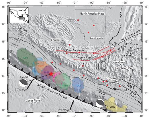
Seismotectonic setting of the study area with subducting slab contours (Hayes et al.2012). Coloured regions show the approximate rupture zones of M > 7 shallow thrust subduction earthquakes since 1900 digitized from White et al. (2004) and Franco et al. (2005). The Mw = 7.3 2012 El Salvador slip area is from Geirsson et al. (in preparation). Focal mechanisms (but not rupture zones) of the M = 7.4 2012 August 27 earthquake off the coast of El Salvador and the M = 7.4 2012 November 7 Champerico earthquake studied herein are also shown. Red circles show the locations of all 19 continuous GPS stations used in this study.
Here, we use observations from 19 GPS sites in northern Central America to determine best-fitting solutions for coseismic and postseismic slip associated with the 2012 Champerico earthquake, including first estimates of the magnitude and depth range of fault afterslip triggered by a subduction thrust earthquake along the Guatemala trench segment. Our analysis complements the seismological study of Ye et al. (2013), who inverted regional seismic and teleseismic P waves from the earthquake to determine a coseismic slip solution. Their results suggest that coseismic slip of up to 6.6 m at depths of 20–25 km released most of the seismic energy within a relatively compact area, with the remaining seismic moment released by lesser slip (0.7 m) along a broader region updip from the region of high slip. As part of our analysis, we examine whether the location and distribution of the seismologically derived slip are consistent with our geodetic measurements of the coseismic elastic deformation at locations immediately onshore from the earthquake.
2 PLATE TECTONIC SETTING
At the location of the 2012 Champerico earthquake, the Cocos Plate subducts beneath the North America and Caribbean Plates at respective velocities of 77 ± 3 mm yr−1 towards N32°E ± 1° and 71 ± 3 mm yr−1 towards N21°E ± 1° (Fig. 1; DeMets et al.2010), roughly orthogonal to the trench (DeMets 2001). The subduction interface must thus accommodate ∼7–8 m of thrust motion per century through some combination of thrust earthquakes and possibly creep. Since 1900, nearly all of the Middle America subduction interface along the coast of El Salvador, Guatemala and southern Mexico has ruptured in earthquakes with magnitudes between 7 and 8 (Fig. 1). Seismic observations of nearly all these earthquakes are non-existent or of poor quality (White et al.2004). Little therefore is known about the seismogenic behaviour of the interface, including the typical depth and magnitude of thrust earthquakes, the extent of their rupture zones, their recurrence intervals, and whether earthquakes are accompanied by significant afterslip.
Seismological and geodetic studies have defined several first-order characteristics of the subduction interface in this area. One important characteristic is progressive steepening of the dip of the subducting Cocos Plate to the southeast (Fig. 2b; Burbach et al.1984), corresponding to the transition from Cocos–North America Plate subduction in the northwest to Cocos–Caribbean Plate subduction in the southeast (Fig. 2a). Although the effects of the transition on thrust earthquake frequency, depths and magnitudes are poorly understood, GPS observations indicate that the transition coincides with strong coupling below southern Mexico, where the slab dip is shallower and North America is the upper plate (Correa-Mora et al.2008; Franco et al.2012) to weak coupling below El Salvador and Guatemala, where the slab dip is much steeper than below southern Mexico and the upper plate is the Central American forearc sliver (Lyon-Caen et al.2006; Correa-Mora et al.2009; LaFemina et al.2009; Franco et al.2012). The 2012 Champerico earthquake occurred near the transition between the strongly and weakly coupling interfaces (Fig. 2a).
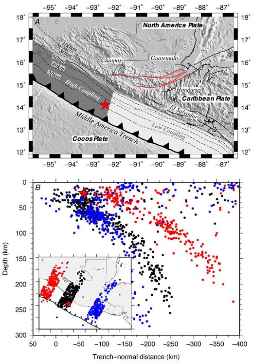
(a) Fault coupling along the Middle America trench from Franco et al. (2012). (b) Vertical earthquake cross-section for three 50-km-wide transects of the Coco Plate subduction interface. One transect spans the North America Plate boundary (red), a second spans the Caribbean forearc sliver (blue), and a third is in the transitional region (black). Earthquake hypocentres are teleseismic relocations of earthquakes in the period from 1960 to 2008 (Engdahl et al.1998). The 2012 Champerico earthquake centroid (red star) in both panels is from the Global CMT catalogue (Dziewonski et al.1981; Ekström et al.2012).
3 DATA
3.1 GPS network and observations
The data used for our modelling are from 23 continuous GPS stations in Guatemala, El Salvador and southern Mexico, 19 of which were operating during the 2012 Champerico earthquake and four of which were installed to monitor postseismic deformation (sites CHPO, MAZ0, QUE1 and SMHO; Fig. 3). The majority (12) of the stations are operated by Guatemala's Instituto Geográfico Nacional. The others are operated by a variety of national agencies and geophysical investigators. All 23 sites consist of modern dual-frequency P-code GPS receivers and antennas.
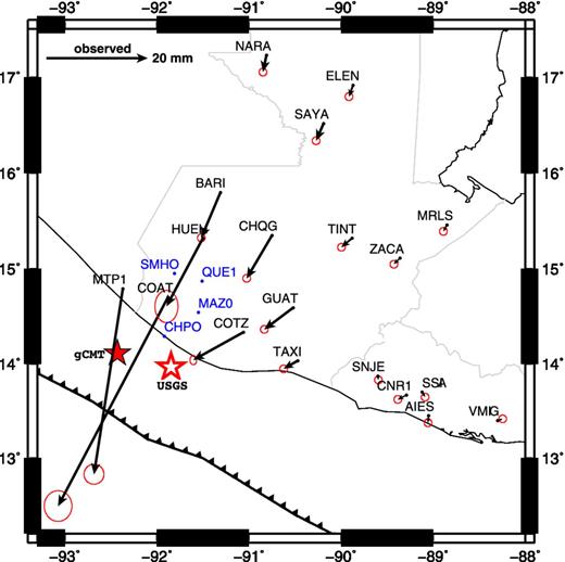
Observed horizontal GPS site offsets and 1-D, 1-σ uncertainties for the 2012 Champerico earthquake. Sites with blue labels but no offsets were installed after the earthquake for monitoring postseismic deformation.
GPS data from these stations were processed with Release 6.1 of the GIPSY software suite from the Jet Propulsion Laboratory (JPL). No-fiducial daily GPS station coordinates were estimated using a precise point-positioning strategy (Zumberge et al.1997), including constraints on a priori tropospheric hydrostatic and wet delays from Vienna Mapping Function (VMF1) parameters (http://ggosatm.hg.tuwien.ac.at), elevation dependent and azimuthally dependent GPS and satellite antenna phase centre corrections from IGS08 ANTEX files (available via ftp from sideshow.jpl.nasa.gov), and corrections for ocean tidal loading (http://froste.oso.chalmers.se). Wide- and narrow-lane-phase ambiguities were resolved for all the data using GIPSY's single-station ambiguity resolution feature (Bertiger et al.2010).
All daily no-fiducial station location estimates were transformed to ITRF2008 (Altamimi et al.2011) using daily seven-parameter Helmert transformations from JPL. Spatially correlated noise between stations is estimated from the coordinate time-series of well-behaved continuous stations from within and outside the study area and is removed from the time-series of all sites (Márquez-Azúa & DeMets 2003). Noise in the daily 3-D site locations averages 1.5 mm in the northing and easting components and 3–4 mm in the vertical component.
Fig. 3 shows the estimated coseismic offsets. At sites COAT, COTZ, HUEH and MTP1, where rapid postseismic deformation was measured, we estimated the post-earthquake site locations from only 24 hr of data after the earthquake. At stations more distant from the earthquake, where no significant postseismic deformation was detected, we estimated the post-earthquake site locations from 5 to 14 d of observations after the earthquake. The largest measured offsets were at COAT (47 ± 3 mm), MTP1 (37 ± 1 mm) and HUEH (15 ± 3 mm), which are all located near the rupture zone (Table 1). The pattern of coseismic offsets is consistent with that expected for a shallow-thrust earthquake, with the site offsets pointing towards the offshore rupture zone and decreasing in magnitude with distance from the rupture zone. No clear pattern of vertical offsets was observed, indicating that vertical deformation from the earthquake was below the vertical resolution of the GPS data.
Overall, 11 continuous GPS sites recorded significant postseismic deformation (Fig. 4). Seven sites were operating during the earthquake and four were added within two weeks of the earthquake (locations indicated by blue symbols in Fig. 3). Results from modelling the postseismic deformation recorded at these 11 sites are described in Section 5.
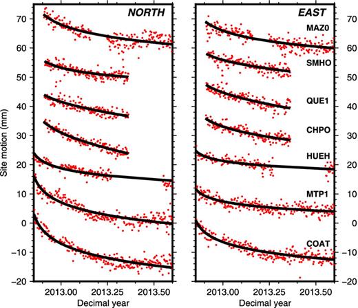
Postseismic position time-series for selected GPS stations, northing and easting components, and best-fitting logarithmic decay models (black lines) from the time-series inversions described in the text. Circles show daily GPS position estimates. Stations are labelled in Fig. 3. Linear trends corresponding to the secular station movements in ITRF08 have been removed at each site.
4 COSEISMIC SLIP SOLUTION
4.1 Inverse method and assumptions
We estimate the distribution of slip during the Champerico earthquake from a standard inversion of the 3-D coseismic offsets and their uncertainties assuming that the deformation occurs on a fault embedded in a homogeneous, elastic half-space (Okada 1985). We discretized the subduction interface near the Champerico earthquake into 42, ∼30 × 30 km rectangular subfaults (Fig. 5a). We adopt subduction contours from Hayes et al. (2012) to approximate the along-strike and downdip geometry of the subducting plate. In Section 4.2, we describe results that suggest our geodetic slip solution is robust with respect to plausible variations of the subduction interface geometry.
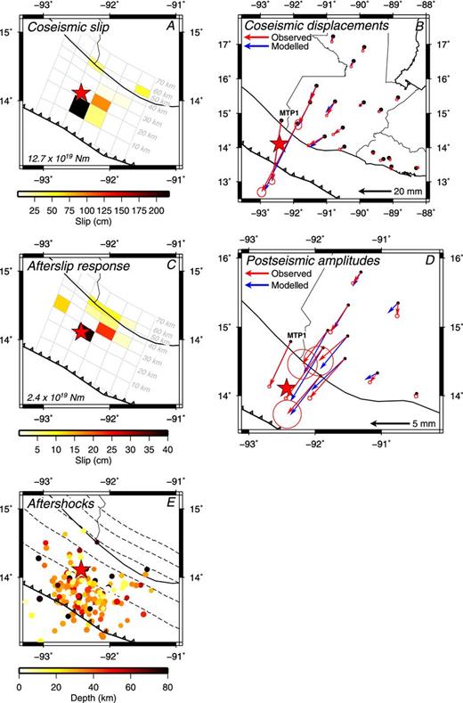
(a) Best-fitting coseismic slip solution of the 2012 Champerico earthquake. (b) Modelled and observed horizontal coseismic GPS site displacements and associated 2-D, 1-σ offset uncertainties for the 2012 earthquake. (c) Best-fitting postseismic afterslip solution for six months after the Champerico earthquake. (d) Modelled and observed horizontal postseismic time-series amplitudes and associated 2-D, 1-σ offset uncertainties. (e) Two-week aftershocks with depths for the Champerico earthquake from the seismic database of the Instituto Nacional de Sismología, Vulcanología, Meteorología e Hidrología in Guatemala. The red star indicates the Champerico earthquake location from the Global CMT catalogue (Dziewonski et al.1981; Ekström et al.2012).
The inversion procedure enforces smoothing and sense-of-slip (non-negativity) constraints using a bounded-variables least-squares algorithm (Stark & Parker 1995) to avoid physically implausible solutions. The algorithm minimizes ∥Gm−d∥2 for all elements of m greater than zero.
During different parts of the analysis, we also use the model resolution (Rm = G♯G) and data resolution (Rd = GG♯) matrices, where G♯ = (GTG + α2FTF)−1GT. The former matrix specifies the resolution of the slip solution as a function of location on the fault plane, whereas the diagonal elements of Rd, which are known as the data importance, specify the relative amount of information that individual data contribute to the solution.
4.2 Coseismic slip solution: preferred and alternative estimates
Fig. 5(a) shows the best-fitting coseismic fault-slip solution for an optimized rake of 82°, where 90° constitutes pure dip-parallel thrusting. The most slip (∼220 cm) occurred on a fault patch between 10 and 20 km depth and close to the earthquake centroid (red star in Fig. 5a). Lesser slip (90 and 30 cm) extended downdip to 30 km depth northeast of the main slip area (Fig. 5a). The geodetic moment estimated from the best-fitting slip solution, 12.7 × 10¹⁹ N m (Mw = 7.36) for a shear modulus of 40 GPa, agrees well with the seismological moments of 14.5 × 10¹⁹ N m (Mw = 7.41) from the Global CMT catalogue (Dziewonski et al.1981; Ekström et al.2012), 13.3 × 10¹⁹ (Mw = 7.34) from the U.S.G.S. and 15 × 1019 N m from Ye et al. (2013). The three highest-slip patches, all between depths of 10 and 20 km, account for most (∼85 per cent) of the estimated moment. We interpret lesser slip along several deeper, isolated fault patches as artifacts of the inversion that modestly improve the fits at nearby high importance sites, with no physical significance and no impact on our solution.
The north, east, and vertical offsets at the 19 GPS sites are well fit by the best-fitting slip solution (Fig. 5b and Table 1), with a weighted rms (wrms) misfit of 1.0 mm and reduced chi-square of 2.57. The offsets at the four sites nearest the rupture zone (MTP1, COAT, COTZ and HUEH), where small variations in the location or magnitude of the modelled slip cause large changes in the predicted site offsets and hence model fit, have a summed data importance of 85.4 per cent (Table 1). By implication, the best-fitting slip solution is determined principally from those four offsets. That the best-fitting slip solution fits the other 15 site offsets so well (Fig. 5b) indicates that the data and solution are highly consistent.
As a blind test of the slip solution described above, a subset of the coauthors estimated an alternative slip solution in parallel with the analysis described above. The alternative slip solution imposes a simpler form on the coseismic slip, consisting of a single fault patch with uniform coseismic slip (Fig. S2b). The strike (293°), dip (29°) and rake (78°) of the fault patch were fixed to seismologically derived estimates from Ye et al. (2013). The dimensions and location of the slip patch were varied to optimize the fit. The best-fitting solution consists of ∼2.8 m of slip along a rectangular fault area that is 42 km along-strike, 20 km downdip, and has its upper edge at a depth of 20 km (location indicated by the black rectangle in Fig. S2b). The location, dimensions and slip amount are similar to those for our preferred solution. The seismic moment of this solution, 8 × 10¹⁹ N m, is roughly 60 per cent smaller than for our preferred solution and is smaller than any of the seismologic estimates. The wrms misfit is ∼1.5 mm, roughly 50 per cent larger than for the preferred solution. Given the simplicity of this solution, we are encouraged by its good agreement with both the data and our preferred solution and conclude that to first-order, our estimate of the coseismic slip is robust (Table S1).
4.3 GPS network resolution and robustness of the slip solution
Given the one-sided distribution of the GPS sites with respect to the offshore rupture, we used a variation of the checkerboard test to evaluate how accurately the GPS offsets resolve the location and magnitude of offshore slip. The slip solutions described above and the seismologic slip solution of Ye et al. (2013) indicate that most slip during the Champerico earthquake was concentrated in a compact rupture zone. We thus elected to test how well the slip magnitude and location can be recovered for a hypothetical thrust earthquake in which 1 m of downdip slip occurred along two adjacent slip patches (Figs S3–S5). For a series of hypothetical earthquakes that are located progressively farther down the subduction interface (locations shown in panels A1–G1 of Figs S3–S5), we used DISL to predict synthetic displacements at each GPS benchmark and perturbed the synthetic offsets with random Gaussian noise assuming GPS uncertainties of ±1 mm for the north and east offset components and ±2.5 mm for the vertical offset components. Inversions of the noisy synthetic data for each model correctly recovered the slip-patch locations for depths between 10 and 60 km, independent of the assumed rupture depth, and slip magnitudes (panels B3–F3 of Figs S3–S5). Slip at the depths recovered from our observed coseismic offsets is thus well resolved by the GPS network. Hypothetical slip at depths shallower than 10 km or below 60 km could not however be recovered (panels A3 and G3 of Figs S3 and S5). Our ability to resolve slip at these depths is thus limited.
5 POSTSEISMIC DEFORMATION: NOVEMBER 2012 TO MAY 2013
Deformation after a large subduction earthquake represents a superposition of a site's long-term interseismic motion and transient deformation from an unknown combination of fault afterslip and viscoelastic flow in the lower crust and upper mantle. We first evaluate whether viscoelastic flow triggered by the earthquake could be responsible for most or all of the postseismic deformation. We then invert the postseismic GPS time-series in a two-stage process to constrain the location and magnitude of fault afterslip.
5.1 Viscoelastic deformation
We first test the hypothesis that all or most of the postseismic deformation (e.g. Fig. 4) occurred in response to viscoelastic flow that may have been triggered by the Champerico earthquake. To approximate the viscoelastic deformation, we applied Visco-1-D software (version 3) of Pollitz (1997) to our preferred coseismic slip solution (Fig. 5a) assuming a spherical, layered earth model that approximates the properties of continental crust. We approximated the properties of continental crust with a modified version of crustal model M1 of Hearn et al. (2013), which consists of an elastic layer from the surface to a depth of 25 km, a Maxwell viscoelastic layer from 25 to 30 km, a stronger layer from 30 to 50 km, and Maxwell viscoelastic material everywhere below 50 km. Unlike Hearn et al., who assumed respective viscosities of 3 × 10¹⁹ and 3 × 10¹⁸ Pa·s for the lower crust and mantle, we assign a viscosity of 5 × 10¹⁷ Pa·s to these two layers in order to approximate a maximum likely viscoelastic response during the months after the earthquake. We adopt this viscosity from Hu & Wang (2012), who conclude from their analysis of short-term postseismic deformation from the 2004 Sumatra earthquake that the mantle below the upper plate behaves as a biviscous Burgers body with a transient short-term viscosity of 5 × 10¹⁷ Pa s and a long-term, steady state viscosity of 10 19 Pa s.
Fig. 6 shows the predicted viscoelastic deformation onshore from the Guatemala earthquake for the above rheological model and our preferred coseismic slip solution. During the first eight months after the earthquake (the period spanned by our postseismic analysis), the predicted site motions are to the south and west (Figs 6a and b), in accord with the directions recorded by continuous GPS sites in the region. The predicted displacements are however too small. For example, at site COAT near the rupture zone, the viscoelastic model predicts motion that is no more than ∼30 per cent of that observed after correcting COAT's observed motion for its long-term interseismic movement. The viscoelastic model also incorrectly predicts slow, postseismic subsidence at COAT (Fig. 6c), whereas no significant vertical motion was recorded.
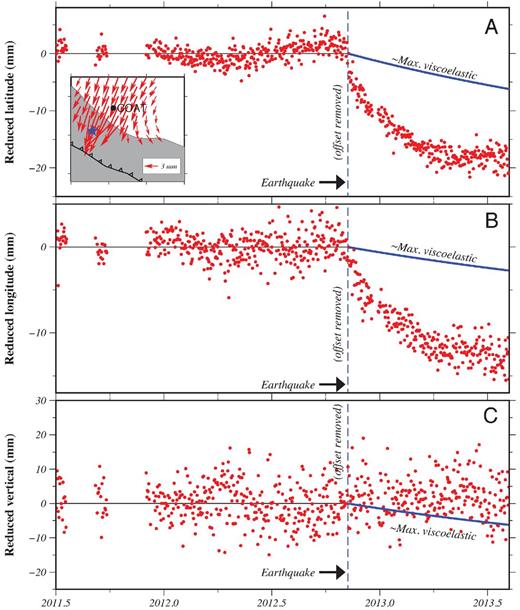
Reduced position time-series for GPS site COAT and viscoelastic deformation (blue lines) predicted for an Earth structure that maximizes the viscoelastic response to the Champerico earthquake (see text). Panels (a), (b), and (c), respectively show the north, east and vertical daily site positions (red symbols) reduced by the slope that best fits the observations from the years before the earthquake. Systematic departures of the postseismic daily positions from the interseismic site motion (black line) measure the postseismic deformation. The coseismic offset has been removed for clarity. The maximum predicted viscoelastic deformation (blue line) is much less than the observed deformation; fault afterslip is thus responsible for most of the deformation. Red arrows in the inset map show the cumulative predicted viscoelastic movement during the first eight months after the earthquake.
We conclude that viscoelastic deformation triggered by the earthquake was at most a minor component of the postseismic deformation and focus hereafter on the more likely explanation, that fault afterslip caused most of the postseismic deformation during the period examined here.
5.2 Inversion for best-fitting postseismic surface deformation
Using eq. (3), we inverted the daily 3-D site positions at all 11 GPS sites where postseismic deformation was detected to estimate the temporal decay constant β, the amplitudes Ai, the intercepts u0i and if necessary, secular velocity components vi at each site for the north, east and vertical components. We limited the time spanned by the observations to the first six months after the earthquake to increase the likelihood that the deformation samples fault afterslip rather than viscoelastic deformation. At seven sites, we estimated the interseismic velocity components from a year or more of measurements before the earthquake and fixed their velocity terms during the inversion. At the four stations that were installed after the earthquake, we estimated the interseismic velocities vi along with the amplitudes Ai and initial positions u0i.
Fig. 4 shows the fits of the resulting optimized model to selected GPS position time-series. Reduced chi-square is 1.0 for the best-fitting model, indicating that the GPS time-series are fit within their estimated uncertainties for deformation that obeys eq. (3). The normalized misfit is minimized for a decay constant of 10 d (Fig. 7a).
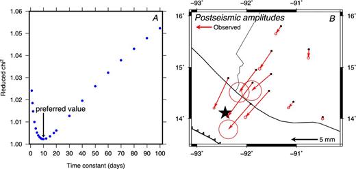
(a) Variations in the normalized misfit to postseismic GPS position time-series as a function of different assumed time constants for logarithmically decaying deformation (see text). Fits to the time-series for the 11 stations that recorded postseismic deformation are optimized for a time constant of 10 d. (b) Amplitudes of postseismic deformation from a joint inversion of all 11 station time-series for a decay constant of 10 d. Uncertainties are 1-σ and are propagated from the observations.
5.3 Inversion results for postseismic fault afterslip
The spatial pattern of postseismic deformation amplitudes estimated from our inversion of the postseismic station time-series (Fig. 7b and Table 1) shares many characteristics with the pattern of coseismic offsets (compare Figs 5b and d). In both cases, sites move to the SSW towards the rupture zone, with amplitudes/offsets that diminish with distance from the rupture area. The site directions after the earthquake (Fig. 5d) however point more uniformly to the SSW than during the earthquake (Fig. 5b), particularly for sites near the coast. Specifically, the direction of postseismic motion at site MTP1 is rotated ∼15° clockwise from the coseismic direction at that site (Figs 5b and d), possibly indicating that some afterslip occurred directly offshore from MTP1, where no coseismic slip occurred.
Using methods described in Section 4.1, we inverted the 33 north, east and vertical site amplitudes and their uncertainties (Table 1) to estimate the pattern of afterslip on the subduction interface and optimal direction for the slip. Fig. 5(c) shows the best-fitting afterslip solution for a rake of 82°, for which the fit is optimized. More than 70 per cent of the postseismic slip occurred at depths of 20–30 km or immediately downdip (Fig. 5c). In contrast, ∼90 per cent of the coseismic slip was concentrated at the same depth or updip from the epicentre (Fig. 5a). Our best-fitting afterslip solution includes some afterslip at depths of 30–60 km at most locations that are directly offshore from the GPS sites (Figs 5c and d). The earthquake thus may have triggered afterslip along a broader area of the subduction interface than ruptured during the earthquake.
The wrms misfit of the best-fitting afterslip solution is 0.6 mm with reduced chi-square of 11.8. The amplitudes for sites CHPO, COAT, MAZ0 and MTP1 contribute ∼80 per cent of the data importance and thus dominate the slip solution, a fact attributable to their proximity to the zone of afterslip.
Six months after the earthquake, the cumulative energy released by the afterslip was 2.4 × 10 19 N m, ∼20 per cent of the main shock and equivalent to a Mw = 6.9 earthquake. Afterslip was largely concentrated at the same depth or downdip from the earthquake (Fig. 5c). In contrast, the earthquake aftershocks were concentrated mostly updip from the hypocentre (Fig. 5e). Afterslip and aftershocks therefore appear to have affected different areas of the subduction interface.
5.4 Resolution of and constraints on the afterslip location
The number and distribution of GPS stations that recorded postseismic deformation is significantly smaller and more compact than for the earthquake, thereby implying lower resolution of the source of postseismic afterslip. We therefore repeated the resolution tests described in Section 4.3 using the 11 GPS stations that recorded postseismic deformation. Tests of a variety of assumed slip locations and imposed slip magnitudes suggest that hypothetical afterslip greater than 50 cm is well resolved at most depths below 10 km. In contrast, slip at the shallowest level in our mesh (0–10 km), where many aftershocks occurred (Fig. 5), cannot be resolved if its magnitude is under 50 cm.
We evaluated how well the GPS data constrain the depth of afterslip by comparing the fits of three alternative models for afterslip, one of which restricts all afterslip to depths shallower than 30 km (Fig. 8c) , a second of which restricts afterslip to depths from 10 to 40 km (Fig. 8d), and the third of which restricts afterslip to depths below 40 km (Fig. 8e). The first and last of these fit the data poorly, with respective values for reduced chi-square that are ∼65 per cent greater and an order-of-magnitude greater (Fig. 8a) than for the best-fitting afterslip solution. The deep subfault model is rejected at much greater than the 99 per cent confidence level based on an F-ratio comparison of their fits to that of the preferred solution. The model that forces afterslip to occur between depths of 10 and 40 km increases the misfit by ∼20 per cent relative to the preferred solution (Figs 8a and d ), constituting a marginally significant increase in misfit (97.7 per cent confidence level).
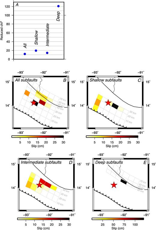
(a) Variations in fits to postseismic deformation amplitudes as a function of four different configurations of subfaults shown in (b)–(e). Configuration in (b) repeats the least-constrained configuration, corresponding to Fig. 5(c). The configuration in (c), which forces all slip onto subfaults above depths of 30 km, increases the misfit by a factor of six (see a). Configurations that permit slip at intermediate depths (d) and below depths of 40 km (e) also increase the misfit. Configuration (e), which greatly increases the misfit, is excluded at high significance levels.
The above results thus exclude models in which most or all of the afterslip was located updip from the earthquake, where numerous aftershocks were recorded (Fig. 5e), or in which afterslip occurred exclusively on deeper areas of the subduction interface. Our results instead require that afterslip occurred at the same depth or deeper than the main shock.
6 DISCUSSION
6.1 Comparison to a seismologic slip solution
Ye et al. (2013), who estimate the distribution of slip during the Champerico earthquake from regional seismic and teleseismic P waves, find that coseismic slip of up to 6.6 m occurred (Fig. 9a), with most of the seismic energy concentrated in a compact area at depths of 20–25 km and lesser slip (0.7 m) along a broader region updip from the region of high slip. Their slip solution is more concentrated, farther updip, has higher peak slip and is located ∼50 km ESE from both our preferred solution and the CMT centroid (compare Figs 5a and 9a). Below, we examine the significance and cause of these discrepancies.
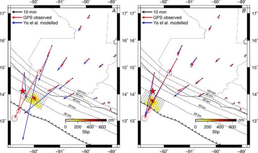
Comparison of our measured GPS offsets (red arrows) and those predicted by Ye et al.'s (2013) coseismic slip solution (blue arrows). (a) Subfaults and slip solution from Ye et al. (2013) in their original location. (b) Fit of seismic slip solution when centroid is translated 51 km west of its initial position in (a).
Fig. 9(a) compares the coseismic offsets that are predicted by the Ye et al. (2013) seismic slip solution to the offsets we measured at each of the 19 GPS sites. Nearly all of the predicted offsets are larger than the observed offsets and are rotated systematically anticlockwise at the sites near the rupture (Fig. 9a), where the predicted deformation directions are sensitive to any mislocation of the modelled slip on the subduction interface. The wrms misfit, 6.4 mm, is a factor of six larger than for our preferred solution (wrms = 1.0 mm). The seismological slip solution at the location used by Ye et al. (2013) is strongly rejected by the GPS data (Fig. 9a).
As a test, we systematically translated the Ye et al. slip solution towards the earthquake epicentre while reevaluating its misfits to the GPS data. Translating the seismic slip solution 51 km westward to the location shown in Fig. 9(b) greatly improves the fit (Fig. 9b). The slip centroid for the translated solution (Fig. S2c) coincides with the centroid of our preferred solution (Fig. S2a) and the wrms misfit for the translated solution is 1.8 mm, much closer to that for our preferred solution. Most of the misfit thus comes from a suboptimal location of the original seismologic slip solution rather than a mischaracterization of how the slip was distributed.
The relatively good fit of the translated seismologic slip solution to the GPS offsets is instructive. That a solution with more concentrated slip and 2–3× higher peak slip amplitude fits the data nearly as well as our preferred solution suggests that the geodetic and translated seismologic solutions constitute possible end-members for the Champerico earthquake slip distribution. Both indicate that coseismic rupture extended no deeper than 30 km, with most energy release occurring at depths of 15–30 km. The seismologic slip solution suggests that lesser slip may have extended up to the trench (Fig. 9a), in agreement with the distribution of locally recorded earthquake aftershocks (Fig. 5e).
GPS station information, earthquake offsets, and postseismic amplitudes.
| Coseisimic offsets | Postseismic amplitudes | |||||||||||||||
|---|---|---|---|---|---|---|---|---|---|---|---|---|---|---|---|---|
| Site | East (mm) | North (mm) | Vertical (mm) | Imp. | East (mm) | North (mm) | Vertical (mm) | |||||||||
| Lat.oN | Lon.oE | Height (m) | Obse±1σ | Modele | Misfite | Obsn±1σ | Modeln | Misfitn | Obsv±1σ | Modelv | Misfitiv | per cent | Obse±1σ | Obsn±1σ | Obsv±1σ | |
| MTP1 | 14.791 | − 92.368 | 52.70 | − 5.7±1.3 | − 5.5 | − 0.2 | − 36.7±1.3 | − 36.8 | 0.1 | 4.3±7.0 | − 1.0 | 5.3 | 35.2 | − 2.7±0.1 | − 5.6±0.1 | − 0.7±0.5 |
| COAT | 14.702 | − 91.885 | 425.96 | − 21.7±1.8 | − 20.1 | − 1.6 | − 41.3±2.0 | − 40.9 | − 0.4 | 1.8±2.0 | − 3.5 | 5.3 | 24.5 | − 4.7±0.1 | − 6.4±0.1 | − 0.3±0.5 |
| COTZ | 14.335 | − 91.058 | 302.24 | − 9.9±1.3 | − 9.4 | − 0.5 | − 5.5±2.0 | − 6.7 | 1.2 | 1.5±7.6 | − 0.5 | 2.0 | 15.0 | − 0.9±0.1 | − 1.2±0.1 | − 1.1±0.5 |
| HUEH | 15.328 | − 91.503 | 1874.88 | − 7.2±1.5 | − 7.4 | 0.2 | − 13.5±2.1 | − 14.7 | 1.2 | − 1.9±5.9 | − 0.7 | − 1.2 | 10.7 | − 2.2±0.2 | − 3.4±0.2 | 0.5±0.6 |
| BARI | 15.802 | − 91.315 | 1459.13 | − 3.8±0.5 | − 4.1 | 0.3 | − 9.0±0.5 | − 8.6 | − 0.4 | − 1.9±2.0 | 0.1 | − 2.0 | 3.4 | − 1.0±0.1 | − 1.4±0.1 | 0.5±0.5 |
| TAXI | 14.035 | − 90.465 | 45.02 | − 2.8±0.5 | − 2.2 | − 0.6 | − 1.6±0.5 | − 1.8 | 0.2 | 0.5±2.0 | − 0.9 | 1.4 | 3.3 | − 0.1±0.2 | − 0.3±0.2 | − 0.9±0.5 |
| CHQG | 15.350 | − 90.752 | 1278.40 | − 5.0±0.5 | − 5.8 | 0.8 | − 8.5±0.5 | − 7.0 | − 1.5 | − 5.1±1.1 | − 0.2 | − 4.9 | 2.9 | − 0.1±0.2 | − 1.6±0.2 | 1.0±0.6 |
| GUAT | 14.590 | − 90.520 | 1519.87 | − 5.7±0.5 | − 5.7 | 0.0 | − 4.3±0.5 | − 4.1 | − 0.2 | 0.8±2.0 | − 0.8 | 1.6 | 2.2 | – | – | – |
| TINT | 15.318 | − 89.875 | 114.61 | − 2.1±0.5 | − 3.1 | 1.0 | − 1.8±0.5 | − 2.7 | 0.9 | − 3.1±2.0 | 0.0 | − 3.1 | 0.5 | – | – | – |
| SAYA | 16.520 | − 90.192 | 141.85 | − 1.5±0.5 | − 2.0 | 0.5 | − 3.4±0.5 | − 3.0 | − 0.4 | − 0.3±2.0 | 0.3 | − 0.5 | 0.4 | – | – | – |
| NARA | 17.228 | − 90.810 | 71.31 | − 0.7±0.5 | − 1.3 | 0.6 | − 3.3±0.5 | − 2.8 | − 0.5 | 3.3±2.0 | 0.3 | 3.0 | 0.4 | – | – | – |
| SNJE | 13.868 | − 89.601 | 1656.96 | − 1.8±0.5 | − 0.9 | − 0.9 | − 4.3±0.5 | − 0.7 | − 3.7 | 6.2±2.0 | − 0.6 | 6.8 | 0.3 | – | – | – |
| ELEN | 16.916 | − 89.868 | 116.02 | − 0.8±0.5 | − 1.5 | 0.7 | − 2.3±0.5 | − 2.2 | − 0.1 | − 4.4±2.0 | 0.2 | − 4.6 | 0.3 | – | – | – |
| ZACA | 15.113 | − 89.356 | 130.31 | − 1.2±0.5 | − 2.0 | 0.8 | − 1.2±0.5 | − 1.6 | 0.4 | − 1.5±2.0 | − 0.1 | − 1.4 | 0.2 | – | – | – |
| CNR1 | 13.670 | − 89.289 | 924.44 | − 1.7±0.5 | − 0.5 | − 1.2 | − 0.9±0.5 | − 0.4 | − 0.5 | − 2.0±2.0 | − 0.6 | − 1.4 | 0.2 | – | – | – |
| MRLS | 15.462 | − 88.850 | 44.15 | − 0.7±0.5 | − 1.5 | 0.8 | − 1.3±0.5 | − 1.2 | − 0.1 | − 4.2±2.0 | 0.0 | − 4.2 | 0.1 | – | – | – |
| SSIA | 13.697 | − 89.117 | 624.39 | 0.6±0.5 | − 0.5 | 1.1 | − 1.0±0.5 | − 0.4 | − 0.6 | − 5.7±2.0 | − 0.5 | − 5.2 | 0.1 | – | – | – |
| AIES | 13.447 | − 89.050 | 35.82 | − 2.1±0.5 | − 0.3 | − 1.8 | − 7.3±0.5 | − 0.3 | − 6.9 | 2.0±2.0 | − 0.5 | 2.5 | 0.1 | – | – | – |
| VMIG | 13.396 | − 88.305 | 374.85 | − 1.8±0.5 | − 0.2 | − 1.6 | − 6.3±0.5 | − 0.2 | − 6.1 | 2.2±2.0 | − 0.3 | 2.5 | 0.0 | – | – | – |
| CHPO | 14.294 | − 91.915 | 9.86 | – | – | — | – | – | – | – | – | – | – | − 4.2±1.3 | − 4.8±1.3 | 12.5±4.2 |
| MAZ0 | 14.537 | − 91.550 | 342.00 | – | – | – | – | – | – | – | – | – | – | − 2.2±0.2 | − 3.4±0.2 | 0.5±0.6 |
| QUE1 | 14.871 | − 91.515 | 2386.53 | – | – | – | – | – | – | – | – | – | – | − 3.7±1.3 | − 3.1±1.3 | 12.5±4.4 |
| SMHO | 14.953 | − 91.808 | 2412.13 | – | – | – | – | – | – | – | – | – | – | − 3.2±1.3 | − 4.2±1.3 | 15.0±4.4 |
Notes: Coseismic offsets are estimated using methods described in text. Postseismic amplitudes are calculated from eq. (3). Modelled offsets are for the preferred slip distribution shown in Fig. 5(a). ‘Imp.’ gives the summed importance for the north, east, and vertical coseismic offsets per site and represents the relative contribution of the site offset to the best slip solution (see text).
6.2 Middle America trench: implications for the Guatemala segment
Our analysis and that of Ye et al. (2013) clearly indicate that the 2012 Champerico earthquake was a subduction thrust earthquake that is typical of other strongly coupled segments of the Middle America trench/Mexico subduction zone. Unlike the exceptionally shallow 1992 Nicaragua slow earthquake (Satake 1994) and 2012 El Salvador thrust earthquake (Ye et al.2013; Geirsson et al., in preparation), the Champerico earthquake ruptured the subduction interface at depths of 15–35 km, typical of numerous other thrust earthquakes along strongly coupled segments of the Mexico subduction zone. Contrary to the 2012 El Salvador earthquake, whose seismic wave spectra and long-lasting rupture duration resemble those of the 1992 slow Nicaragua earthquake (Ye et al.2013), the Champerico earthquake seismic-source spectra were normal for a subduction earthquake (Ye et al.2013). By inference, strong coupling appears to extend along the Guatemala segment at least as far southeast as the Guatemala/Chiapas border, in accord with GPS results reported by Franco et al. (2012). Whether the subduction interface remains strongly coupled even farther to the southeast offshore from Guatemala is unknown. The GPS stations that were used by Franco et al. (2012) to constrain the location of the offshore transition from strong to weak coupling were spaced too far apart to define whether the along-strike transition occurs gradually or suddenly. Either seems possible given that factor-of-two variations in coupling over distances of several tens-of-km are well documented along the Mexico subduction zone (Correa-Mora et al.2008) and under the Nicoya Peninsula in Costa Rica (Feng et al.2012). GPS measurements at more closely spaced stations along Guatemala's Pacific coast will resolve this in the next few years.
7 CONCLUSIONS
Inversions of GPS-recorded coseismic offsets caused by the Mw = 7.4 2012 Champerico subduction-thrust earthquake indicate that coseismic fault-slip was concentrated at depths of 10–30 km and extended along strike by ∼50 km, in good accord with the locations and distribution of aftershocks associated with the earthquake. Peak slip of ∼2 m occurred near 14.0°N, 92.5°W, close to the centroid estimated by the Global CMT project. The geodetic moment of 12.7 × 10 19 N m (Mw = 7.4) also agrees well with most seismologic estimates. SSW station movement towards the trench dominated transient postseismic deformation recorded by 11 GPS sites near the rupture zone. Forward modeling of the expected viscoelastic deformation based on our best-fitting geodetic solution suggests that it constitutes no more than ∼30 per cent of the total postseismic deformation. Futher modelling indicates that fault afterslip caused most of the transient deformation, occurred mostly downdip from the main shock, and released energy equal to ∼20 per cent of the 2012 rupture (Mw = 6.9) within 6 months of the earthquake. The seismological derived slip solution of Ye et al. (2013), which has more concentrated slip and higher peak slip values, fits our coseismic GPS offsets well if the slip solution is translated to the approximate location of our geodetic slip solution.
This work was funded by NSF grant EAR-1144418 (DeMets) and is based upon work supported by the National Science Foundation under grant EAR-1042906 to UNAVCO. We thank Universidad Mariano Galvez and Universidad San Carlos for logistical support. Data critical for this work were procured from El Instituto Geográfico Nacional (IGN). Postseismic measurements at sites MAZ0, SMH0, QUE1, and CHP0 were possible thanks to funding from INSU-CNRS in France and the help of the French Embassy in Guatemala City. Figures were produced using Generic Mapping Tools software (Wessel & Smith 1991).
REFERENCES
SUPPORTING INFORMATION
Additional Supporting Information may be found in the online version of this paper:
Figure S1. Comparison of coseismic offsets for the Champerico earthquake from the primary analysis (black arrows and Table 1) and the alternative analysis (red arrows and Table S1).
Figure S2. Measured horizontal coseismic offsets and predictions of three solutions for the coseismic slip. (a) The preferred geodetic solution (Fig. 5a and Table 1 from the main document). (b) Alternative geodetic solution with ∼2.8 m of slip on a single fault. (c) Seismologically-derived slip solution of Ye et al. (2013) after translating the solution 51 km to the west from the solution location indicated by Ye et al. (2013).
Figure S3. Results from slip-patch resolution test. Coloured squares show fault patches where 1 m of slip is either imposed (panels A1–G1) or slip is estimated via inversions of synthetic coseismic offsets created with the imposed solutions (panels A2–G2 and A3–G3). Red star indicates the epicentre of the 2012 Champerico earthquake. Further details are given in the main and supplementary documents.
Figure S4. See caption to Fig. S3.
Figure S5. See caption to Fig. S3.
Table S1. Coseismic observed offsets and estimated offsets from preferred and alternative solutions described in main document. (Supplementary Data)
Please note: Oxford University Press is not responsible for the content or functionality of any supporting materials supplied by the authors. Any queries (other than missing material) should be directed to the corresponding author for the paper.
