


Abstract
Temporal changes in seismic anisotropy can be interpreted as variations in the orientation of cracks in seismogenic zones, and thus as variations in the stress field. Such temporal changes have been observed in seismogenic zones before and after earthquakes, although they are still not well understood. In this study, we investigate the azimuthal polarization of surface waves in anisotropic media with respect to the orientation of anisotropy, from a numerical point of view. This technique is based on the observation of the signature of anisotropy on the nine-component cross-correlation tensor (CCT) computed from seismic ambient noise recorded on pairs of three-component sensors. If noise sources are spatially distributed in a homogeneous medium, the CCT allows the reconstruction of the surface wave Green's tensor between the station pairs. In homogeneous, isotropic medium, four off-diagonal terms of the surface wave Green's tensor are null, but not in anisotropic medium. This technique is applied to three-component synthetic seismograms computed in a transversely isotropic medium with a horizontal symmetry axis, using a spectral element code. The CCT is computed between each pair of stations and then rotated, to approximate the surface wave Green's tensor by minimizing the off-diagonal components. This procedure allows the calculation of the azimuthal variation of quasi-Rayleigh and quasi-Love waves. In an anisotropic medium, in some cases, the azimuth of seismic anisotropy can induce a large variation in the horizontal polarization of surface waves. This variation depends on the relative angle between a pair of stations and the direction of anisotropy, the amplitude of the anisotropy, the frequency band of the signal and the depth of the anisotropic layer.
1 INTRODUCTION
Seismic anisotropy has a key role in the study of strain and stress fields in the Earth. Indeed, on a large scale, the origin of anisotropy (Montagner et al.1998) might be due to the alignment of the crystallographic axes of anisotropic minerals when subjected to a strain field or to aligned cracks (Crampin 1987), or to fluid inclusions, or under the influence of a stress field. As a consequence, the orientation of the anisotropy induced will be parallel to the direction of the stress or strain field that arises through these different processes. Another cause of large-scale anisotropy, and specifically of transverse isotropy with a vertical symmetry axis, is the superposition of thin layers, for wavelengths that are significantly larger than the layer thickness (Backus 1962). In this study, we are interested in seismic anisotropy that is induced by the alignment of cracks in a stress field.
Many methods are used by seismologists to study anisotropy in seismogenic zones, which involve measuring its effects on the propagation of seismic waves. One of these is shear wave splitting (SWS; Vinnik 1977; Crampin et al.1980; Silver & Chan 1991; Zhang et al.2007; Liu et al.2008), a phenomenon that occurs when a polarized shear wave penetrates an anisotropic medium and splits into two S waves. Naturally, as with any other technique, SWS has limitations. Indeed, SWS depends on the occurrence of local earthquakes, and it turns out to be difficult to sample all three directions, as most of the shear waves produced by these earthquakes propagate almost vertically. These limitations to the monitoring of seismic anisotropy can be alleviated by using cross-correlations of continuous ambient noise between each pair of stations in a network of stations, according to the three components of vertical (Z), east and north, rotated into vertical (Z), radial (R) and transverse (T).
The cross-correlation tensor (CCT) computed between two three-component (Z, R, T) seismograms at two different receivers (A, B) is an estimation of the transfer function (Green's function) between these receivers. The CCT has nine components that represent all of the possible cross-correlations between the three component signals recorded at the two receivers. For a homogeneous random distribution of noise sources, the CCT represents the impulse response of the Earth between these two stations. In practice, however, the CCT is dominated by surface waves. Unlike the vertically propagating shear waves that are used for SWS, surface waves propagate horizontally. This allows the measurement of the horizontal seismic properties in the shallow crust.
Since their application to seismology in 2004, the use of the ZZ components of the CCT has enabled the imaging of seismic velocity subsurface structures from seismic ambient noise. The monitoring of seismic velocity changes, which might be related to stress changes in seismogenic zones, has also been demonstrated, with computation of the relative traveltime shift between a perturbed and a reference ZZ for each station pair (Brenguier et al.2008).
Another technique is based on the investigation of the off-diagonal terms of the CCT: ZT, TZ, RT and TR. Indeed, for a random distribution of seismic sources, these non-diagonal terms are null in an isotropic medium. However, in an anisotropic medium, they are no longer null; that is, the polarization plane of quasi-Rayleigh waves is deviated with respect to the isotropic case, and the polarization of quasi-Love waves is no longer in the horizontal plane. The surface wave polarizations are no longer parallel or perpendicular to the direction of propagation. Their directions are slightly deviated, which creates quasi-Rayleigh and quasi-Love waves (Crampin et al.1980). If the CCT is rotated to minimize the off-diagonal components with the optimal rotation algorithm (ORA) code (Roux 2009), the deviation anomaly angles (ψ, δ) at both receivers (A and B) can be retrieved. These four angles are defined by the horizontal polarization anomaly at receivers A and B (ψA, ψB) and the vertical polarization anomaly at receivers A and B (δA, δB). These anomaly angles inform us about the anisotropic properties in the medium or the inhomogeneity of sources (Durand et al.2011).
In this study, a numerical investigation is performed, knowing that there is no analytical solution for surface wave propagation in such anisotropic medium with horizontal symmetry axis. Our goal is to investigate the physical conditions that can give rise to rotation of the polarization of seismic surface waves, and it is the most efficient way to measure the azimuthal rotation that is linked to anisotropy. The objective is to correctly interpret the observations made by Durand et al. (2011) for large variations in surface wave polarization (>20°) within a limited zone of the seismic array, and before and after the 2004 Parkfield earthquake. In the following, the technique based on the optimal rotation of noise cross-correlation is detailed and then tested on synthetic seismograms that are computed with a spectral element method [the RegSEM code, for the regional spectral elements method, as detailed in Cupillard et al. (2012)].
2 SYNTHETIC EXPERIMENTS
![Representation of the HTI medium, the 72 sources, and the 72 stations. This figure is not drawn to scale [Δ(R1 − R37) = 10 km and Δ(S1 − S37) = 332 km]. ψα is the azimuth of the fast direction of anisotropy fixed in the east–west direction, ψS is the azimuth of incidence of the source, and ψR is the azimuth of the pair of stations. All angles are measured in degrees in a clockwise direction from the north line.](https://oup.silverchair-cdn.com/oup/backfile/Content_public/Journal/gji/201/2/10.1093/gji/ggu470/2/m_ggu470fig1.jpeg?Expires=1716401601&Signature=pUeceJ8lDKMDJyBW8dyUrMRQmFR97fec4IrBRUa29fnZSTIonlXP1Kzx3L8Hop5Ojw6nNriL44ndqTC1OGzu~SHImXXO21STe1nKAQIyOO1NBH3RmRhOnbsDWoKV4ghTAcBkvSLAUdRyTj8WSPakrOJVu3QIETg0oe-RieGpOgmQJvXd7Qdms~vFt5X0V~g1m-80kHd~or8Eiq~E0svFJVmnCSt56krXK4YkORgO0S2kCrw3tKg984l~edISxZeru9XDb82iKAQqbLTCk-C0MjOf3J3RYZ3Ujy9GkvYW5jxotmPtQHhHxdV-9TclN2HI~M8RTjAN9y4ZSI31pRJGhQ__&Key-Pair-Id=APKAIE5G5CRDK6RD3PGA)
Representation of the HTI medium, the 72 sources, and the 72 stations. This figure is not drawn to scale [Δ(R1 − R37) = 10 km and Δ(S1 − S37) = 332 km]. ψα is the azimuth of the fast direction of anisotropy fixed in the east–west direction, ψS is the azimuth of incidence of the source, and ψR is the azimuth of the pair of stations. All angles are measured in degrees in a clockwise direction from the north line.
We start by considering the case of an impulse force at the source location, so the transformation of the Rayleigh wave into a quasi-Rayleigh wave will be correctly observed, limiting the influence of the Love wave. That way we can clearly explore the effect of anisotropy on the propagation of Rayleigh waves only. Fig. 2 shows that the signal on the radial and vertical components of the synthetic seismograms is dominated by Rayleigh waves in isotropic and anisotropic media.
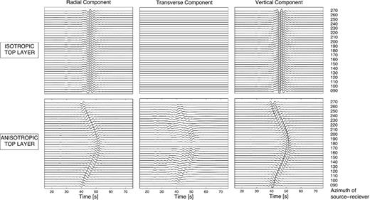
Radial, transverse and vertical components for the source incidences, going from azimuth 90° to 270°. The source–station pairs that correspond to the different azimuths are formed from sources Si and receivers Ri located on the circles shown in Fig. 1; for example, for azimuth 135°, the source is S10 and the receiver is R10. As indicated, the top three panels are seismograms computed in an isotropic medium, and the bottom three panels are seismograms that were computed in a medium where the velocity anisotropy is ±10 per cent and the thickness d of the top anisotropic layer is 10 km. In the isotropic medium, there are only Rayleigh waves on the radial and vertical components. In the anisotropic medium, and for waves that propagate along the fast and slow axes (90°, 180°), there are also only Rayleigh waves on the radial and vertical components, which propagate in the symmetry planes of the medium. However, for the other source incidences, a signal appears on the transverse component, which is due to the creation of quasi-Rayleigh wave in the anisotropic medium. Moreover, in the anisotropic medium, the group velocity decreases as the incidence of the source approaches the slow axis, and increases as the incidence of the source approaches the fast axis.
Fig. 2 also shows that a weak signal appears on the transverse component for waves that propagate in an anisotropic medium, which is primarily due to the deviation of the Rayleigh wave into a quasi-Rayleigh wave. There is also a small faster signal that might be related to quasi-Love waves. The anisotropy affects the group velocity: there is a decrease in the group velocity when the azimuth of incidence of the source ψS approaches the north-south direction. This is the minimum for a wave that propagates perpendicular to the direction of anisotropy, where the velocity is slowest, and the group velocity is maximum for a wave propagating along the direction of anisotropy. Another observation is the difference between the velocities along the fast axis and the slow axis, which is 20 per cent, the percentage of anisotropy in the top layer (±10 per cent).
3 THE METHOD
3.1 Cross-correlation of seismic data
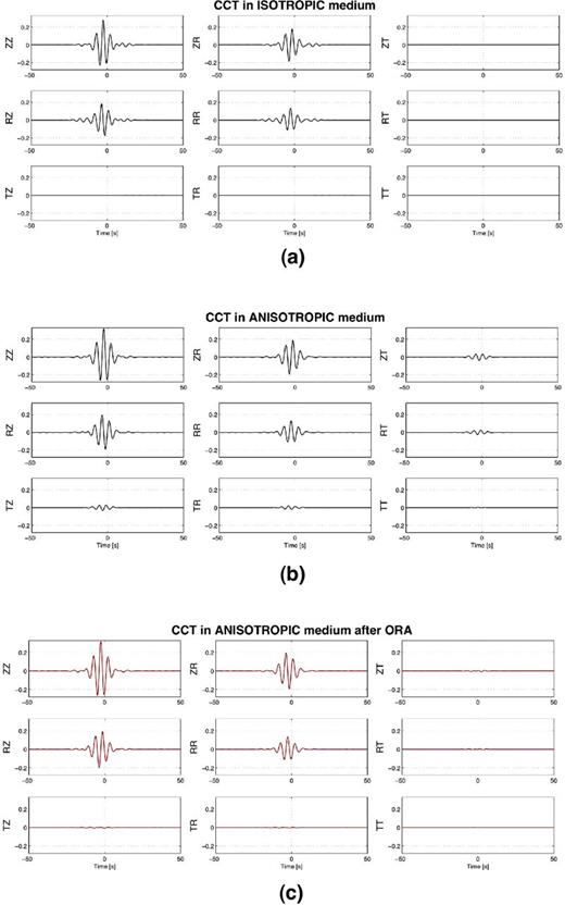
(a) CCT in an isotropic medium for a single source and a receiver pair of azimuth 110°. (b) CCT for the same receiver pair in an anisotropic medium, where the velocity anisotropy is ±10 per cent. (c) CCT after the application of the ORA. The frequency band in all cases is 0.15–0.25 Hz. The source is aligned with the pair of stations, and the CCTs are represented in the ZRT coordinate system, where the radial axis is parallel to the incidence of the source.
3.2 Application of the optimal rotation algorithm
The ORA was first introduced in Roux (2009), to deal with directive incident noise for seismic noise tomography. In fact, in order to perform passive seismic imaging, station pairs that do not align with the noise direction should be thrown away, since they provide a biased traveltime through noise correlation (Roux 2009). The main objective of ORA is to allow each station (from a specific station pair, A and B) to freely rotate around both the vertical axis (with the azimuth angle ψ) and the radial axis (with the tilt angle δ) and to align with the incident noise direction (Fig. 4), by minimizing the four off-diagonal terms ZT, RT, TZ and TR of the CCT computed between these two stations (Fig. 3c). This way, the number of station pairs that can be used in the traveltime tomography inversion is increased.
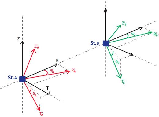
Azimuths ψA and ψB and tilts δA and δB used in the ORA.
The ORA is then used to determine the set of angles that minimizes the components ZT, RT, TZ and TR of the original CCT, by finding the minimum misfit parameter. Indeed, the less M is, the closer the tensor is to the Rayleigh wave Green's tensor.
Thus, even if the station pair is originally misaligned with the noise incidence, the four off-diagonal terms ZT, RT, TZ and TR, will be zeros after the ORA rotation, if we assume the medium is isotropic. In this way, it is possible to correct the station pairs that do not align with the noise direction by rotating both stations and to provide unbiased tomography measurements through noise correlation (Roux 2009). However, Fig. 3(b) shows that in the case of an anisotropic medium, components ZT, RT, TZ and TR still have nonzero values; that is, the polarization plane of the quasi-Rayleigh and quasi-Love waves is slightly deviated by horizontal and vertical angles, with respect to the polarization plane of the Rayleigh and Love waves in the isotropic medium.
In this case, the value of the ORA azimuthal rotation angle that minimizes the components ZT, RT, TZ and TR of the CCT is equal to the angle that aligns the station pairs with the noise source incidence and an additional angle that is due to the deviation of the Rayleigh and Love waves in the anisotropic medium (Fig. 3c). Our goal is to investigate this additional rotation angle that arises due to the anisotropy, by using ORA in cases where the station pairs are aligned with the source incidence. Therefore, the difference between the azimuthal rotation angles given by ORA (ψA, ψB) and the azimuth of the source incidence gives the anomaly angles that are associated with the deviation of the surface waves in an anisotropic medium at both stations. Here ψA is equal to ψB because the source is aligned with the stations pair, hence the anomaly angle is the same at both stations. The case of omnidirectional source distribution is presented in Fig. 5, for which the anomaly angle becomes independent of the source incidence.
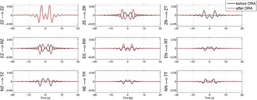
Representation of the CCT before (black) and after (red) the ORA, for a receiver pair of azimuth 135°. This is a case of multidirectional far sources in a ±10 per cent anisotropic medium.
4 RESULTS
In the numerical experiment, the CCT is computed for each pair of stations, as stations Ri and Ri + 36, which are aligned along the diameter of the inner circle shown in Fig. 1 (dots). The Rayleigh wave sources are distributed in the far field of the receivers in a circle of radius 166 km, as shown in Fig. 1 (stars). The polarization anomaly angles ψP and δP computed using the ORA are functions of ψR. We note that the tilt δP is always negligible, as the medium is HTI, and hence we study only the azimuthal polarization anomaly ψP. Fig. 6 shows the variation of the horizontal polarization anomaly (ψP) for different frequency bands. In the model, the depth of the anisotropic layer is 10 km, and the amplitude of anisotropy is ±10 per cent.
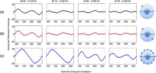
Variations in the horizontal polarization anomaly angle ψP as a function of ψR for three cases: a point source (ψS = ψR) (black), two symmetrical sources (red), and the stack of the CCTs of all of the sources (blue). In this model, the depth of the anisotropic layer is 10 km, and the anisotropy is ±10 per cent.
First of all, the point sources are studied one by one, and we consider the case where the azimuth of the source ψS is equal to the azimuth of the station pair ψR. For the direction source stations parallel or perpendicular to the direction of anisotropy (fast or slow axis for propagation of the signal in a symmetry plane), there is no transverse component and no effects of anisotropy, except through the propagation velocity. Hence, the terms ZT, RT, TR and TZ of the CCT are null, and so the angle given by the ORA is equal to the azimuth of the station pair. On the contrary, as soon as the angle between the direction source stations and the direction of anisotropy is different from 0° or 90°, the anisotropy affects the wave propagation and the polarization anomaly can be computed. Looking at the results for a single point source and two symmetrical sources, a first observation is that ψP appears to be highly dependent on the frequency band, and basically varies with 2Ψ and 4Ψ (Fig. 6 a). This frequency dependence is due to the presence of anisotropy in the shallow layer.
Note also that the azimuthal variation of the tilt δP (the vertical polarization anomaly angle) has small values comparing to ψP. The tilt δP, can be ignored, as expected for a HTI medium. This will not be the case for a tilted transversely isotropic medium, which might be the case in subduction zones.
The third case is a simulation of a homogeneous azimuthal distribution of far-field sources by adding the contribution of all of the sources on the external circle. For each station pair, a stack of the individual CCTs obtained from the 72 sources is almost equivalent to the CCT obtained in a uniform source distribution, which leads to the reconstruction of the surface wave Green's tensor. We then observe the variation of the horizontal polarization anomaly angle ψP as a function of the azimuth of the station pair ψR. In this case, the variations of ψP are larger and vary with 2Ψ at lower frequencies. Between 0.17 and 0.25 Hz, the sign of ψP begins to reverse, with 2Ψ and 4Ψ variations (Fig. 6c).
Based on the study of Tanimoto (2004), theory shows that the polarization of surface waves propagating in an anisotropic medium contains 2Ψ and 4Ψ azimuthal dependance, similar to the phase velocity variations. In particular in an HTI medium, it is possible to detect azimuthal dependance of 2Ψ and 4Ψ in the azimuthal polarization of surface waves. 4Ψ variations are basically related to Love waves, whereas 2Ψ variations are related to Rayleigh waves that seem to be dominating at lower frequencies where sources are homogeneously distributed.
Another observation is the difference between the results with a single point source and a homogeneous distribution of sources. Indeed, the present study shows that the sum of the CCTs in an anisotropic medium is different from the sum in an isotropic one. In an isotropic medium, contributions to the CCTs from anti-symmetric sources (Si+k – Si−k, where i is from 1 to 72 and k is from 1 to 35 and they define the location of the source as in Fig. 1) cancel each other out in the summation. The result would be a surface wave Green's tensor equivalent to the tensor built by the sum of two CCTs associated with the two symmetrical sources on either side of the station pair. However, in an anisotropic medium, the sum is different. These same contributions have different arrival times, so they do not vanish after the summation.
Finally, note that the amplitude of the polarization anomaly ψP can be very large (reaching 20° and more), and it depends on many parameters, such as the amplitude of anisotropy and the frequency of the signal.
As mentioned previously, the final CCT obtained after the rotation using the ORA is the one that corresponds to the lowest misfit. Fig. 7 shows the value of the final misfit given by the ORA as a function of ψR, for each CCT rotated and horizontal polarization anomaly computed. In Fig. 7, the three cases from Fig. 6 are represented, including a single point source (ψS = ψR), two symmetrical sources, and a stack of the CCTs of all of the sources. The value of the final misfit for all of the cases is <1 per cent of the total energy, which validates the use of the ORA.
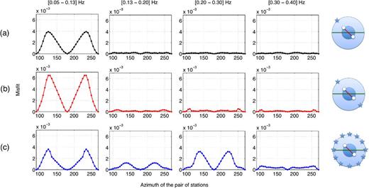
Final misfit obtained from the ORA as a function of ψR, and corresponding to the computation of the horizontal polarization anomaly in the three cases shown in Fig. 6: a point source (ψS = ψR) (black); two symmetrical sources (red); and a stack of the CCTs of all of the sources (blue). As shown in the figure, the misfit should be less than 1 per cent of the total energy.
5 DISCUSSION
In the crust, the occurrence of an earthquake affects and rotates the stress tensor. Consequently, the temporal rotation of the stress tensor induces rotation of the crack distribution (Crampin 1981), and hence a change in the direction of the anisotropy (ψα), which induces temporal changes in the polarization of the surface waves propagating in the medium (ψP). ψP depends on the relative angle between the azimuth of the station pair and the direction of the anisotropy, ψR − ψα = Δψ. In ‘real life’, we search for temporal changes in ψα(t) by monitoring ψP(t), knowing ψR. In our numerical experiments, we investigated the variation of ψP with fixed ψα in the east–west direction, and we considered various ψR. The positions of the source and the station pair vary, spanning the whole range of azimuthal incidences relative to the direction of anisotropy. In this way, it is possible to observe the azimuthal variation of the horizontal polarization anomaly angle ψP, measured using the ORA, as a function of ψR, the azimuth of the path. Therefore spatial variations observed with synthetic tests can be interpreted in terms of temporal variations observed with real data, given the equivalence between the two.
The results of the numerical experiments combined with the theory of anisotropic wave propagation show that the variation of the horizontal polarization of a surface wave propagated in an anisotropic medium (and here we consider a HTI medium) greatly depends on several parameters. These parameters are the amplitude of anisotropy, the depth and thickness of the anisotropic layer, the distance between the source and the receivers, and especially the azimuth of the source and the pair of receivers relative to the azimuth of anisotropy. Another parameter is the homogeneity of the source distribution. The CCT converges toward the Green's tensor if the source distribution is uniform. This is rarely the case; that is, in the region of California, the main source of noise originates along the Californian coast at short periods, but from the northern Atlantic at long periods, as shown by Stehly et al. (2006).
The goal of this paper is not to demonstrate the Green's function reconstruction between two receivers, which was done in earlier papers for any level of heterogeneity in the propagation medium (Campillo & Roux 2014). The goal here is to search for the effect of anisotropy from an interferometric approach. In fact we deal with far-away sources and we chose pairs with small interstation distances. That way we have a good coherence between receivers and we study local effects beneath the stations. As in the case of Parkfield (Durand et al.2011), large polarization changes were observed although interstation distances are relatively small. Note also, that the effect of anisotropy on the propagation of surface waves is not cumulative, unlike traveltime measurements. It depends on the anisotropic structure of the medium but not on the distance travelled by the wave.
As a matter of fact, the level of complexity that interests us and that we want to address in this study is the one related to the anisotropic model, and not to the complexity related to the source distribution. Therefore, we use the most favourable cases, an homogeneous distribution of sources as well as directive noise sources as found in Parkfield (Durand et al.2011) but still aligned with the receiver pair. That is why the azimuthal polarization anomaly at both receivers is the same. If we consider an heterogeneous source distribution, the only difference is that the polarization anomaly will be different at each receiver. In real case scenario, the heterogeneity of the noise source distribution (and its variation in the time associated to seasonal changes) should not be a problem since, using beamforming technique (Roux 2009; Durand et al.2011), we can compute the temporal variation of the incidence of the dominant source and then retrieve it from the polarization anomaly given by ORA. A comparison between temporal variation of the polarization anomaly and the seasonal variation of the source incidence is essential to the analysis in order to identify changes of polarization due to anisotropy and the ones due to a source incidence change. Nevertheless, seasonal variations of the source incidence and anisotropy changes do not evolve on the same characteristic time. Hence, a rapid and large change that extends on a relatively small period of time could not be due to a source incidence variation.
The multitude of parameters involved in the creation of ψP makes it difficult to find a unique interpretation of the variation of ψP. Our numerical experiment shows that ψP is highly sensitive to the presence of anisotropy, even for a very shallow anisotropic layer, which is probably not sufficient to affect other physical parameters that produce SWS. In all cases, the angle ψP can be very large (>20°). The large values of ψP with respect to δt/t measured for SWS make it easier to consider monitoring ψP. Indeed, δt/t of SWS can be very small, and even not measurable in some cases; for example, if the anisotropy is weak or if the thickness of the anisotropic layer is small. Another advantage of measuring ψP is that monitoring this parameter is possible, as is monitoring seismic anisotropy and observing temporal changes using continuous ambient seismic noise data. As for SWS, it depends on the occurrence of earthquakes, and a temporal change in δt/t cannot be observed, as we cannot observe azimuthal changes in SWS in the synthetic experiments presented here. Finally, the last advantage of using CCTs is to deal with n*(n − 1)/2 measurements for n stations, unlike for n measurements with SWS.
As classically done in ambient noise monitoring, the δt/t measurement can also be performed on the surface waves extracted from the CCT. The relative traveltime change (δt/t) measured on the ZZ component of the CCT of the numerical experiments shows a difference of 20 per cent between the δt/t along the slow axis (azimuth 180°) and the fast axis (azimuth 90°; Fig. 8). This value was expected as it corresponds to the velocity difference between the slow axis and the fast axis. However, in practical applications, time delays are not measured on the direct waves extracted from the noise cross-correlations, since the first arrival time delay is subject to seasonal variations. Monitoring relative traveltime is usually performed using the coda of noise cross-correlations (Sabra et al.2005; Brenguier et al.2008). Coda waves are scattered waves that travel large distances and accumulate time delays. Hence, it allows the detection of very small perturbations in seismic velocity. They are also known to be less sensitive to the noise direction than direct waves. On the other hand, the coda is weakly affected by local effects (Planes et al.2014) as expected from a change of anisotropy during an earthquake. Finally, note that typical values of measured δt/t in the coda cross-correlations is of the order of 10−3 (Brenguier et al.2008).
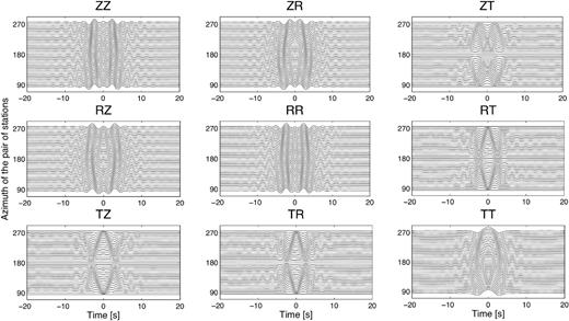
Representation of the nine components of the cross-correlation tensors associated with 37 station-pairs with azimuth going from 90° to 270°. In each panel the bottom signal corresponds to a station-pair of azimuth 90° (parallel to the direction of anisotropy), the middle signal corresponds to a station-pair of azimuth 180° (perpendicular to the direction of anisotropy) and the top signal corresponds to a station-pair of azimuth 270° (parallel to the direction of anisotropy). The source distribution is homogeneous. The difference between the δt/t along the slow axis (azimuth 180°) and the fast axis (azimuth 90°) is 20 per cent.
Durand et al. (2011) observed rapid variations (>20°) of the horizontal polarization of surface waves at stations of the high resolution seismic network at the moment of the 2004 Parkfield earthquake for only a limited part of the San Andreas Fault. These strong and fast changes occurred only ‘in a small zone in the southern portion of the seismic array, near the San Andreas Fault, and above the primary rupture zone of the Parkfield earthquake’.
This study provides a possible, and we believe most likely, explanation of these rapid and large horizontal polarization changes in terms of the anisotropic medium. We also note that even if no fast and significant changes of the surface wave polarization were observed in some areas, this does not necessarily mean that the anisotropy distribution did not change. This can be explained by an unfavourable configuration of stations and source, with respect to the direction of the anisotropy, where the polarization is not highly affected.
The Parkfield region is well instrumented and has been well studied. Geophysicists have carried out continuous measurements of the whole area, and preliminary models of the distribution of cracks and the stress field in the region have been obtained. Therefore, the argument of anisotropy change to explain the fast polarization changes can be verified by the measurements of the stress field changes in the area. These measurements were carried out by Nadeau et al. (2009) in the analysis of unusual earthquake and tremor seismicity at Parkfield. It appears that the large polarization changes observed by Durand et al. (2011) are located in the same zones where Nadeau et al. (2009) found the most important regional shear stress changes. This confirms that strong anisotropy changes can induce such strong horizontal polarization anomalies.
6 CONCLUSION
The noise cross-correlation method is a consistent method for monitoring crustal property changes throughout seismic cycles. The ORA procedure applied to the nine-component CCT between two receivers measures the surface wave polarization anomaly angle. Any temporal change in the polarization anomaly angle might be related to seismic anisotropy and a temporal change in the stress field in the medium that induces a change in the crack distribution. The application of this method to synthetic seismograms confirms the hypothesis that anomalous observations of large and fast variations of surface wave polarization with time can be explained by seismic anisotropy. The next step is to apply the noise cross-correlation method to real data, to monitor stress field changes in different tectonic contexts.
This study is performed in the Seismology Laboratory of Insitut de Physique du Globe de Paris, under the leadership of Jean Paul Montagner and Philippe Roux to whom I would like to express my gratitude for their supervision and guidance. I would like to thank all the co-authors for their collaboration, specially Paul Cupillard for his help with the RegSEM code. The simulations presented in this paper were performed using the Institut de Physique du Globe de Paris Cluster. Many thanks also to Christopher Berrie for the review of the paper.
