Lithospheric architecture of the South-Western Alps revealed by multiparameter teleseismic full-waveform inversion

Summary

1 INTRODUCTION

The Alpine Belt results from the collision between the European margin and the Adriatic margin, initiated during the Paleogene 35 Ma ago as a consequence of the Alpine Tethys closure (Stampfli et al. 2002; Handy et al. 2010). It is nowadays one of the most studied orogenic domains in the world, and therefore an ideal target to understand the deep processes and mechanisms of orogeny. Notably, the Western part of the Alps has preserved its full metamorphic history and has been the cradle of the continental subduction concept, with the discovery by Chopin (1986) of HP-LT coesite-bearing metamorphic rocks in the Dora Maira massif. Even though this concept was already proposed for other tectonic area as the Indu Kush range (Roecker 1982), these rocks were the first indubitable petrological evidence of the burial of the continental crust at depths greater than 90 km (Marchant & Stampfli 1997; Zhao et al.2015).

However, at that time, no clear seismic evidence was available for such a mechanism in the alpine orogeny and the concept of continental subduction was highly debated. While high-resolution tomographic images of the deep lithosphere were lacking, key insights on the upper-lithospheric structure of the Western Alps were inferred from various geophysical studies. Notable features like the Ivrea body (early revealed by gravity anomalies) were interpreted as uplifted mantle materials within the upper crust. The crustal velocities and the Moho discontinuity inferred from the prominent ECORS-CROP seismic reflection profiling in the late 1980s suggested a mantle wedge intruding the Alpine crust located further west from the Ivrea body (Bayer et al. 1987; Nicolas et al. 1990). A reinterpretation of available geophysical knowledge by Schmid & Kissling (2000) attributed this anomaly to a European lower crustal wedge. Nonetheless, seismic details on the deep structure of the south-western part remain sparse (Thouvenot et al. 2007) and as pointed out by Kissling (1993): ‘without imaging techniques independent of assumptions about tectonic and dynamic processes, such as seismic methods, the various models of deep Alpine crustal structure could not be tested and improved.’

This has motivated intense seismic experiments and studies (Kissling et al. 2006). At crustal scale, local earthquake tomography (LET; Paul et al. 2001; Béthoux et al. 2007), sometimes combined with gravity inversion (Vernant et al. 2002), succeed in revealing details of the shallowest structure of the Alpine crust. They notably underlined the extent of a high P-wave velocity anomaly (from 7.4 to 7.7 km s⁻¹) up to 10 km depth interpreted as the Ivrea body and pointed out its Adriatic mantle origin. Nonetheless, the limited aperture of the available seismic arrays restricted the resolution of these tomographic images to the upper crust. More recent LET studies made use of wider seismic arrays (Diehl et al. 2009; Potin et al. 2015) with a larger number of data allowing the inference of crustal structures down to the lower crust. The tomographic model of Diehl et al. (2009) shows an upper to middle crust dominated by the high velocity anomaly associated with the Ivrea body that can be traced down to 45 km depth. In the upper crust, this Ivrea body is surrounded by low velocity anomalies attributed to the Molasse and Po sedimentary basins that are also well-visible on ambient-noise tomography (Stehly et al. 2009). From 30 km depth, they observed reduced P-wave velocities associated with the thick crustal root of the Western Alps.

The upper-mantle structure of the Alps was derived by Lippitsch et al. (2003) from crustal corrected teleseismic P-wave traveltime tomography. Their study revealed fast velocity anomalies interpreted as remnants of subducting slabs from 100 to 300 km depth in the vicinity of the Alpine Belt. They notably observed a change in the subduction regime along the Alpine Belt. In the Western Alps, they denote a gap of fast velocity in conjunction with a slow velocity anomaly, interpreted as a testimony of slab detachment (Davies & von Blanckenburg 1995; von Blanckenburg & Davies 1995) and a related asthenospheric upwelling. However, in Central and Eastern Alps this fast anomaly can be traced from the crust down to 200 km depth with a reverse polarity in the Eastern Alps. The break-off concept has been invoked in the Western Alps to explain magmatic episodes taking place during the Cenozoic (von Blanckenburg & Davies 1995) and later to explain syn-convergence and tardi-orogenic extension in the Western Alps (Sue et al. 1999; Wortel & Spakman 2000) and dynamic topography effects (Fox et al. 2015; Nocquet et al. 2016). It appears as a major process of collision ranges (Wortel & Spakman 2000) and permits to explain the arcuate shape of the Western Alps as well as the deficit of lithospheric material in the upper mantle (Piromallo & Faccenna 2004). Convergence in the Alps implied horizontal shortening about at least 500 km toward the East (Piromallo & Faccenna 2004), however, tomographic models usually image subductions traces down to only 200–300 km depth. Piromallo & Faccenna (2004) proposed that fast velocity anomalies, localized deeper in the mantle transition zone, correspond to lithosphere subducted until the Paleogen, detached between 35 and 30 Myr and piled up at 660 km depth. Quite recently, Zhao et al. (2016a) performed a finite-frequency traveltime tomography of the Alpine range and questioned the slab break-off hypothesis in the Western Alps. Their tomographic image reveals a down dip fast velocity anomaly that can be continuously traced from 70 km down to 300 km depth.

Despite the significant contribution of these tomographic studies, the need to improve the spatial resolution of the lithospheric models of the Alps and to more completely describe their seismic properties remains. To fill this gap, a dense profile of broad-band stations was deployed during the CIFALPS temporary experiment to collect seismological data amenable to new high-resolution seismic imaging techniques (Zhao et al. 2013). A first exploitation of the CIFALPS data by common conversion point migration of the teleseismic P-wave receiver functions has provided the first conclusive seismic image of a subducting continental crust in the Western Alps (Zhao et al. 2015).

The aim of this study is a second attempt to develop new P- and S-wave velocity and density models of the lithosphere of the western Alps from the CIFALPS data with a resolution of the order of the wavelength. We present an application of full-waveform inversion (FWI) on the CIFALPS data to derive 3-D high-resolution P- and S-wave velocity and density models of the lithosphere of the Western Alps and compare them with the migrated image of Zhao et al. (2015).

Beyond receiver function migration, waveform inversion methods are expected to provide quantitative broad-band lithospheric models with a resolution close to the wavelength. Among teleseismic waveform inversion techniques, migration of scattered teleseismic body waves has been first proposed by Bostock et al. (2001), Shragge et al. (2001), Rondenay et al. (2001) and Rondenay et al. (2005). In their approach, the forward problem is linearized with the single-scattering Born approximation and the migration is recast as a ray-based linear waveform inversion accordingly, where the misfit between the recorded and modelled scattered wavefields is minimized in a least-squares sense. In this framework, Bostock et al. (2001) stress the key contribution of the known free-surface reflector as a second-order source of down-going P and S waves. These down-going P and S waves are amenable to reflection from the lithospheric reflectors before being recorded at the surface by the stations. Migration of these backscattered waves provides sharp quantitative images of lithospheric reflectors which are parametrized by P- and S-wave velocity perturbations. An application on the teleseismic data collected during the 1993 Cascadia experiment reveals the geometry of the continental Moho and the oceanic crust of the subduction Juan de Fuca plate (Rondenay et al. 2001).

A natural extension of the former linear waveform inversion is nonlinear FWI, a technique also borrowed from exploration geophysics (Tarantola 1984; Mora 1987; Crase et al. 1990; Pratt 1999). In a similar way to the linear waveform inversion, FWI relies on the principles of generalized diffraction tomography (Devaney 1984; Wu & Toksöz 1987): the gradient of the misfit function is computed by the zero-lag correlation between the recorded and modelled scattered wavefields. The modelled scattered wavefield corresponds to the partial derivative of the wavefield with respect to the model parameters. In scattering migration, the recorded scattered wavefield is separated from the full wavefield during a pre-processing step once and for all, while, in FWI, the recorded scattered wavefield is built on the fly at each iteration by the differences between the full and the modelled seismograms (namely, the data residuals). In FWI, the forward problem is performed without linearization and a nonlinear inversion is performed with a local optimization technique. This implies that the initial earth model at each iteration is updated with the final model of the former iteration. As small-scale features are added in the subsurface models in which seismic modelling is performed over several iterations, the resulting discontinuities can help to more fully account for converted waves and multiscattering during the inversion process.

In its conventional form, FWI seeks to minimize in a least-squares sense the sample-to-sample misfit between the recorded and modelled seismograms. This implies that both traveltimes and amplitudes of all of the arrivals are involved in the misfit function. Alternatively, the sensitivity kernels of the FWI can be modified in order to recast the waveform inversion in a finite-frequency traveltime inversion of the first arrival (Marquering et al. 1999) or selected wave packets (Maggi et al. 2009). This approach, which accounts for amplitudes during seismic modelling for accurate extraction of time delays but removes their imprint in the misfit function, is generally referred to as adjoint tomography by the earthquake seismological community when seismic modelling is performed with full-wave numerical techniques such as the spectral element method (Komatitsch & Tromp 1999). Here, adjoint means a mathematical technique that allows for the efficient computation of the gradient of a functional without forming the sensitivity matrix (see Tromp et al. (2005); Fichtner et al. (2006a,b); Plessix (2006) for a review). An alternative to the adjoint approach is the scattering-integral approach which relies on the explicit computation of the sensitivity matrix (Chen et al. 2007). Several applications of adjoint tomography at regional, continental and global scales have been presented by Tape et al. (2010), Fichtner et al. (2009), Fichtner et al. (2010), Zhu et al. (2012), Fichtner et al. (2013), Zhu et al. (2015) and Bozdağ et al. (2016).

First attempts of teleseismic FWI were performed in 2-D and 2.5-D (Roecker et al. 2010; Pageot et al. 2013; Baker & Roecker 2014) using a frequency-domain implementation of both the forward and inverse problems (Pratt 1999). A frequency domain implementation was used because 2-D seismic modelling can be performed efficiently with Gauss elimination techniques when a large number of sources are processed for a few discrete frequencies (Pratt 1999). Pageot et al. (2013) presented a parametric analysis that highlighted the contribution of the backscattered waves from the free surface to improve the resolution of the imaging as originally pointed out by Bostock et al. (2001). They also show that a fine sampling of the frequencies was required during the inversion to balance the limited scattering angle illumination provided by a few plane wave sources. This prompts them to conclude that a time-domain implementation of FWI was more computationally efficient than the frequency-domain counterpart for teleseismic imaging.

A first feasibility study of 3-D time-domain FWI of teleseismic data has been performed by Monteiller et al. (2015). In their approach, full-waveform modelling is performed for lithospheric targets with a hybrid approach: first, a simulation is performed in a radially symmetric global earth with the Direct Solution Method (DSM) method (Geller & Ohminato 1994) and the wavefield solutions are stored on the edges of the lithospheric target. Second, a grid injection technique is used to propagate the wavefields in the lithospheric target with the spectral-element method from the storage of the DSM solutions at the edges of the computational mesh (Monteiller et al. 2013). Monteiller et al. (2015) illustrate the resolution power of FWI relative to adjoint tomography (namely, phase inversion of the P wavefield contained in a narrow time window centred on the first arrival) to image a simple crustal model with a sharp Moho even when only four teleseismic events are used for inversion. The reliability of FWI for teleseismic application was further demonstrated with an application to real data collected in the framework of the Pyrope experiment across the Pyrénées range (Wang et al. 2016). FWI of five events recorded by 29 stations provided tomographic P- and S-wave velocity models of the Pyrenean lithospheric structure with an unprecedented resolution. Moreover, Wang et al. (2016) showed the consistency between the P- and S-wave velocity models developed by FWI and migrated images inferred from receiver functions.

In this study, we present an application of FWI on the CIFALPS data set following an approach similar to that of Monteiller et al. (2015). A key difference is that we update the density parameter (ρ) in addition to the P- and S-wave velocity parameters (V_p and V_s). In the first section of the paper, we review some methodological aspects of teleseismic FWI. From the analysis of the radiation patterns of waves scattered by elastic heterogeneities, we also provide some insights on the resolution with which V_p, V_s and ρ can be imaged as well as potential leakage between parameters that might impact upon the multiparameter reconstruction. Then, we show the FWI results and discuss their reliability based on a resolution analysis. We conclude with a discussion on the role of the density in teleseismic FWI and the geodynamical implications that can be drawn from our FWI results. Notably, we highlight the FWI potential in recovering a reliable density model of the upper lithosphere that shows clear correlations with regional gravity anomalies. Upper-lithospheric velocity models well delineate known structures of the upper crust, particularly the geometry of the Ivrea body that is clearly connected to the Adriatic mantle. Deeper, models display a clear crust-mantle boundary that dips down to 80–90 km beneath the internal Alps indicating a continental subduction event as a starting of the continental collision. At lower-lithospheric scale, our results give hint of slab detachment and support the assumption of a slab tear in the Alpine Belt.

2 MULTIPARAMETER TELESEISMIC WAVEFORM INVERSION

2.1 Teleseismic full wavefield modelling

Teleseismic experiments deviate from traditional seismic applications such as local earthquake tomography or controlled-source seismology by rather different acquisition geometry. Classically, seismic sensors are located on top of the lithospheric target to be imaged and basically consist of either linear 1-D or sparse 2-D arrays. The special feature of teleseismic configuration arises from the use of passive and distant sources, located several thousands of kilometres away from the target, commonly referred to as teleseismic events (Fig. 1). In this source-receiver geometry, the teleseismic wavefield can fairly be approximated by an incident planar wavefield incoming from outside of the lithospheric target. Such plane-wave configuration leads to a rather uniform illumination of the lithospheric target (in the sense that planar waves do not suffer from geometrical spreading) at the expense of the incidence-angle coverage, which is much narrower and coarser than for point-source acquisition.

Figure 1.

Open in new tabDownload slide

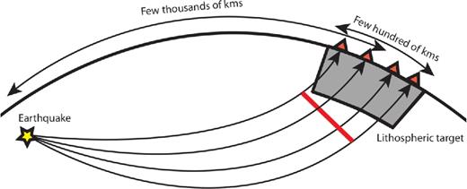
Sketch of the teleseismic configuration.

From the computational perspective, the teleseismic setting raises the issue of the burden associated with the simulation of the teleseismic wavefields in a global earth within the 0.05–1 Hz frequency band. Several approaches based upon hybrid strategies have been proposed to reduce the computational effort of teleseismic wavefield simulation. The governing idea relies on the use of a background wavefield that can be efficiently computed in a simplified earth model and on the efficient computation of either the scattered or the full wavefield after model alteration.

Roecker et al. (2010) introduced the so-called scattered field method (Taflove & Hagness 2005), where the source term of the wave equation is non zero where the background model differs from the model in question. A more affordable strategy for time-domain modelling relies on the so-called total-field / scattered-field grid injection method, which was first proposed to implement point sources in finite-difference simulations (Alterman & Karal 1968; Taflove & Hagness 2005; Monteiller et al. 2013; Masson et al. 2014; Tong et al. 2014). As the scattered-field approach, it also relies on the pre-computation of an incident wavefield in a simplified earth model. However, the storage of the incident wavefield is only required along the outer boundaries of the lithospheric target. This wavefield is then injected within the lithospheric medium by applying a time-dependent boundary condition which accounts both for the incoming incident wavefield and the outgoing wavefield scattered by the lithospheric heterogeneities.

Our approach relies on the 3-D spectral-element method (Komatisch et al. 1998; Komatitsch & Tromp 1999), an efficient method for elastic wave propagation in presence of smoothly varying topography, to simulate the teleseismic wave propagation within the lithospheric target. Unlike Monteiller et al. (2013) who use the DSM method to compute the incident wavefield in a radially symmetric global earth, we use the spectral-element AxiSEM software to compute the 3-D incident wavefield (Nissen-Meyer et al. 2014). AxiSEM is a spectral element solver that allows one to infer 3-D wavefields in a global axisymmetric earth for full-moment tensor sources from four 2-D simulations (Nissen-Meyer et al. 2007a,b, 2008). Its use greatly decreases the memory requirements of simulations performed with DSM in a radially symmetric earth (Takeuchi et al. 2000) or the computational burden of the SPECFEM3D_GLOBE code in a fully 3-D earth (Komatitsch & Tromp 2002).

A cheaper alternative would have been to use a F-K method (Kennett 1983; Zhu & Rivera 2002; Tong et al. 2014) under the assumption that the wavefield reaching the lithospheric target is planar. However, this approach would have prevented the modelling of later arrivals as PcP as well as the pP and sP free-surface reflections. Even if these later might be accounted for through the estimation of a source wavelet, this procedure, which relies on the assumption that the velocity structure is known, can generate significant leakage between the source estimation and the lithospheric parameter updates. Moreover, the plane-wave approximation might not be acceptable at smaller epicentral distances. For all these reasons, we favour a modelling approach that generates global wavefields as realistic as possible in the time window involved in the inversion.

Another advantage of the AxiSEM method is to rely on the same discretization scheme than the one used to perform seismic modelling in the lithospheric target: an SEM method using fourth-order polynomials on hexahedric elements for spatial discretization together with a second-order Newmark time integration scheme. Hence, its use mitigates the imprint of the numerical noise generated during the wavefield injection.

2.2 Inverse problem

While the gradient (3) indicates the direction of greatest ascent and depends on first derivatives of the misfit function, the Hessian is based on second derivatives of the misfit function and accounts for its curvature. The Hessian is of particular interest for FWI, since it deconvolves the gradient from limited bandwidth effects and removes the imprint of wavefield amplitudes. In the framework of multiparameter reconstruction, it contributes to mitigating the cross-talk between multiple parameter classes.

Even though the full Hessian cannot be computed easily (Fichtner & Trampert 2011), its action on the gradient can be approached considering limited-memory quasi-Newton (Nocedal 1980; Nocedal & Wright 2006) or truncated Newton (Métivier et al. 2013, 2014) methods. In our study, the Hessian is iteratively approximated by the l-BFGS method, a matrix-free algorithm that estimates the action of the inverse Hessian onto a vector by applying finite-differences over previous gradients and model parameters. The optimization process including the line search is implemented in our code with the SEISCOPE toolbox (Métivier & Brossier 2016).

2.3 High-resolution multiparameter imaging

Traditional seismic imaging methods such as traveltime tomography or receiver function migration techniques are focused on determining perturbations of wave velocities from the kinematic attributes of the seismic wavefield (namely, traveltimes). On the other hand, the use of the waveforms, through the information carried out by traveltimes and amplitudes of forward- and backward-scattered waves, make FWI amenable to reconstruction of second-order parameters such as density (ρ) in addition to the P- and S-wave velocities (V_p and V_s). Inferences on the sensitivity of the wavefield to different parameter classes can be drawn from the radiation pattern of elastic waves scattered by small elastic heterogeneities (Wu & Aki 1985; Tarantola 1986). These radiation patterns represent the amplitude of P and S waves scattered by a point perturbation of one elastic parameter as a function of the scattering angle. These radiation patterns are shown in Fig. 2 for an isotropic elastic medium parametrized by V_p, V_s and ρ. Such patterns give clear insights on the influence of a single parameter onto the data depending on the scattering regime (forward versus backward). Moreover, the overlap of the radiation patterns of different parameters with scattering angles indicates potential trade-off between these parameters. On the one hand, one may want to mitigate these trade-offs by choosing a parametrization that minimizes these overlaps. On the other hand, this strategy might narrow the influence of the parameters with scattering angle, hence degrading the resolution with which parameters are reconstructed.

Figure 2.

Open in new tabDownload slide

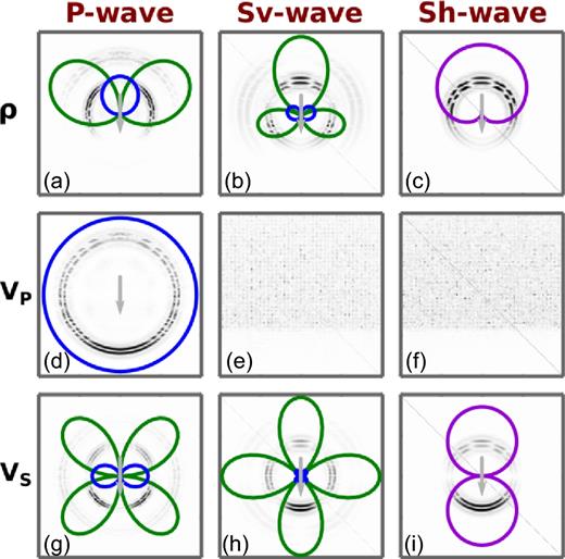
Scattering patterns of elastic waves for the (ρ, V_p, V_s) parametrization. From left to right, each column presents the interaction of a P (a,d,g), Sv (b,e,h) and Sh (c,f,i) incident plane wave with, from top to bottom, a ρ (a–c), V_p (d–f) and V_s (g–i) scattering point. For the seven different interactions, the analytical radiation patterns computed in the framework of the Born approximation (Wu & Aki 1985; Tarantola 1986) are superimposed on the scattered wavefields that have been computed numerically. Arrows indicate the direction of the incident plane wave (black for P wave, red for Sv wave and red–black for Sh wave). Radiation patterns are plotted in blue, green and purple for the P, Sv and Sh scattered modes, respectively.

Limiting our analysis to the (ρ, V_p, V_s) parametrization, a first notable feature is that a V_p scatterer generates only P–P scattering with an isotropic radiation pattern. Therefore, the radiation pattern of V_p has no impact on the resolution with which this parameter is reconstructed (Figs 2d–f): the local resolution of V_p is controlled by the local P wavelength and the range of P–P scattering angles spanned by the acquisition geometry.

In contrast, a V_s perturbation gives rise to P–P, P–S, S–S and S–P scattering, with stronger diffracted S waves relative to the P counterparts (Figs 2g–h). The union of these radiation patterns covers a broad range of scattering angles, that is conducive to a broad-band reconstruction of the V_s parameter if the imprint of all of these scattering modes is significant in the data. Trade-off between V_p and V_s updates is expected to be limited since the V_s parameter generates P–P scattered waves only at intermediate angles with much smaller amplitudes than those generated by V_p. Since the radiation patterns of V_p and V_s should have little influence on the resolution with which they are reconstructed, the resolution of V_s is expected to be superior to that of V_p according to their respective wavelengths.

Similarly to a V_s perturbation, a ρ perturbation generates scattering for the P–P, P–S, S–S and S–P scattering modes. However, a key difference is that ρ mainly scatters waves backward (in the reflection regime). This is especially true for the P–P and S–P modes, while P–S and S–S modes show significant amplitudes at intermediate scattering angles. Overall, this deficit of sensitivity at large scattering angles can limit the ability of FWI to update the long wavelengths of ρ when the (ρ, V_p, V_s) parametrization is used, which can be to some extent balanced by the low frequency content of teleseismic data. This also suggests that the second-order P and S wave sources generated by the free surface might have a leading role in the ρ reconstruction since they generate backscattered waves from the lithospheric reflectors. The ability to image ρ by FWI is therefore prone to decrease rapidly with depth due to the smaller amplitudes of these second-order scattered waves relative to the primary counterparts.

Significant trade-offs are expected at intermediate to small scattering angles between V_p and ρ and between V_s and ρ according to their respective radiation patterns. However, it is worth remembering that V_p and V_s parameters control both the kinematic and the dynamic attributes of seismic waves, while density mostly influences amplitudes. Heuristically, we may think that the long-wavelength reconstructions of V_p and V_s will be primarily tied by the need to fit traveltimes and that amplitudes will play a second-order role in the parameter update, hence limiting the imprint of these parameter trade-offs.

In the remainder of this study, we perform FWI with the (ρ, V_p, V_s) parametrization. Indeed, other combinations of parameters involving P and S impedance or stiffness coefficients can be viewed. A sensitivity analysis of teleseismic FWI to subsurface parametrization will be the aim of a future study.

3 APPLICATION TO THE WESTERN ALPS

3.1 The CIFALPS experiment

The CIFALPS array (for China–Italy–France–ALPS seismic transect) (Zhao et al. 2015) was deployed from June 2012 to September 2013 between the Rhône valley in France and the Po plain in Italy (Fig. 3a). The network was composed of 56 three-components broad-band stations from which 46 formed a 350 km long transect across the Western Alps from SE France to NW Italy (Zhao et al. 2016b). The additional 10 stations were located off-profile 40 km to the North and South to fill gaps in French and Italian permanent networks (network code FR: RESIF (1995); network code GU: University of Genova (1967); network code IV: INGV Seismological Data Centre (1997)). On average, the interstation spacing was less than 10 km for the transect with a 5 km densification in the internal Alps.

Figure 3.

Open in new tabDownload slide

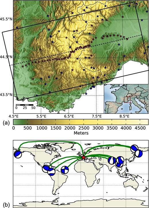
The CIFALPS experiment. (a) Topography of the Western Alps and source–receiver layout of the CIFALPS experiment. Red stars stand for CIFALPS temporary stations while blue stars denote local permanent stations. The black line shows the extent of the model boundaries while the dashed line presents the model profile. (b) The selected nine teleseismic events symbolized by their respective moment tensor solutions.

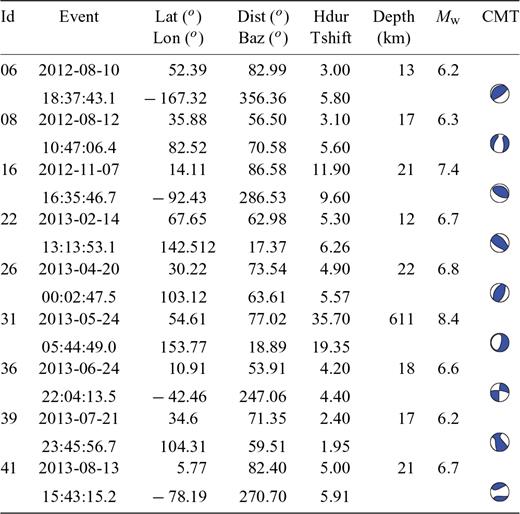
Teleseismic records gave access to a catalogue of 200 earthquakes with magnitude greater than 5.8. We deconvolved each record by its instrumental transfer function, performed a careful inspection of the data set and selected 9 teleseismic events (Fig. 3b) that complied to the following criteria:

• a range of epicentral distances between 30 to 90 degrees,

• hypocentral depths less than 30 km or greater than 200 km,

• a well-discernible spatial coherency of arrivals on vertical and radial records (Fig. 4),

• a high signal-to-noise ratio of individual traces.

Figure 4.

Open in new tabDownload slide

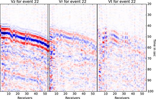
Records of event 22 for the vertical, transverse and radial components. Note some coherent signal hidden within the P-wave coda related to receiver side lithospheric structure (reflections and conversions).

Note that, although some events are quite close, we use them in the inversion to improve the signal-to-noise ratio by summation of redundant information. The lower bound of the first criterion aims to mitigate the imprint in the selected time window of complex shallow multipathing arising outside the lithospheric target, while the upper bound ensures that the direct P wave is the first arrival. The second one controls the complexity of the incident wavefield with respect to source-side multiples: as the event depth increases, the time delay between direct P and pP or sP multiples increases and their travelling paths deviate. In this case, the pP and sP multiples can overprint the useful signals in the selected time window and make the estimation of the source wavelet and subsurface parameters more coupled and sensitive to the error on the hypocentral depth. For very deep events, however, this problem is not a concern since the arrival time of these multiples is far beyond the considered time-window (≈50 s).

Though most earthquakes from the selected catalogue are fairly aligned with the CIFALPS transect, the catalogue covers a broad range of magnitude, distance and spectral content. This is highlighted by the wide range of half-duration in the Global CMT solutions from 2.4 to 35.7 s (Table 1). This can be cumbersome for FWI, particularly at high frequency, in the sense that events will have contrasted spectral contents. Considering the nearly planar nature of teleseismic wavefields, it is crucial for imaging that events cover a wide range of epicentral distances to sample a wide range of incidence angles (Pageot et al. 2013). Typically, teleseismic wavefields are dominated by the incident P and source-side depth multiples (Fig. 4). These are followed by a mixture of lithospheric converted phases such as Ps conversion from the Moho discontinuity, the lithosphere-asthenosphere boundary or 410 and 660 mantle discontinuities. The key challenge of FWI is to extract the information carried out by these secondary signals, which are hidden in the P-wave coda, to enhance the resolution of lithospheric models.

Table 1.

Selected events for teleseismic waveform inversions indicating origin time, location and moment tensor solution from Global CMT project (Dziewonski et al. 1981; Ekström et al. 2012). Half duration (Hdur) and time shift (Tshift) are given in seconds.

Open in new tab

Table 1.

Selected events for teleseismic waveform inversions indicating origin time, location and moment tensor solution from Global CMT project (Dziewonski et al. 1981; Ekström et al. 2012). Half duration (Hdur) and time shift (Tshift) are given in seconds.

Open in new tab

3.2 Full-waveform inversion workflow

Before FWI, we computed and stored the wavefields computed with AxiSEM on the side and bottom boundaries of the lithospheric target. The forward modelling is performed locally with the SEM method on a hexahedral mesh containing 16 000 elements, resulting in 2 million degrees of freedom. The mesh is composed of fourth-order polynomial elements, the size of which is about 10 km. The element size is chosen according to the maximum frequency of the considered propagated seismic signal (0.2 Hz) and the minimum S wave speed so that the size of the elements is of the order of the minimum propagated wavelength. The parameter updates during FWI is performed on a Cartesian grid containing 401 × 201 × 201 grid points spaced 1 km apart in the three spatial directions to facilitate the implementation of smoothing regularization. Then, we estimated a source signature for each individual earthquake by performing a least-squares frequency-domain deconvolution (Pratt 1999) of the recorded vertical seismograms from the synthetic counterparts computed in the initial FWI model. The deconvolution is performed for a 50 s time window that starts 5 s before theoretical onset times of the first P arrival. As initial model we use a smoothed version of the PREM reference model (Dziewonski & Anderson 1981).

Note that the Western Alps topography was not accounted for in our simulations. Although strong topography generates non-negligible surface waves through mode conversions (Monteiller et al. 2013) at high frequencies and can delay the first P arrival and its multiples by a few seconds (less than 3 s), these effects should not be prominent at relatively long periods (more than 5 s). An FWI experiment performed with a synthetic model representative of the Western Alps suggests that not considering the topography during the inversion leads to a noisier density model, probably because density accommodates amplitude errors, and an artificial deepening of reflectors by 1 to 2 km below the highest elevation.

An example of the data fit obtained with the initial model is shown in Figs 5(c)–(e). Interestingly, the first arrival of the synthetic seismograms computed in the initial model is already in fair agreement with the recorded ones for vertical, radial and transverse components. A partial conclusion is that a layered 1-D reference Earth model and automatic moment tensor solutions refined by an estimation of the apparent source wavelet provide the necessary ingredients to predict the low frequency content of the data without any risk of cycle skipping and allows the FWI process to be enable. Nonetheless, slight shifts and amplitude mismatches are visible in the early arrival and more significant waveform differences, whose lateral coherency can be followed from one stations to the next, are showing up for later arrivals testifying the complexity of receiver-side lithospheric structures (Figs 5i–k).

Figure 5.

Open in new tabDownload slide

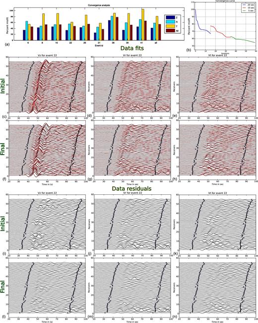
Data fit. (a) Misfit reduction for each component of each event (the right bar shows the misfit function for all components). (b) Overall misfit reduction over iterations. Dash black lines indicate when FWI jumps to a new frequency band (see the text for details). (c–n) Direct comparison between recorded (black) and modelled (red) seismograms for event 22 (Fig. 3c). (c–e) Modelled seismograms are computed in the initial model for vertical (c), radial (d) and transverse (e) components. (f–h) Same as (c–e) modelled seismograms computed in the final FWI model. (i–n) Data residuals computed in the initial (i–k) and final (l–n) FWI models, respectively. Blue stars define the time window used for FWI.

Afterwards, we perform a multiscale FWI of the vertical and radial components by successive inversions of data sets of increasingly high-frequency content with cut-off periods of 20, 10 and 5 s. The optimization process is performed using the l-BFGS algorithm (Nocedal 1980). The step length is computed using the Wolfe conditions (see Métivier & Brossier (2016) or Monteiller et al. (2015) for details on the algorithm). We do not consider any particular initial Hessian H_o except the heuristic one proposed by Nocedal & Wright (2006). Convergence is achieved if the misfit reaches 1 per cent of the initial misfit, if the number of iteration exceeds 100 or if no suitable step length is found. Although transverse component data are accessible and may carry information related to the 3-D lithospheric structure geometry (Cassidy 1992), they are usually influenced by anisotropic effects from the lithospheric medium (Frederiksen & Bostock 2000) and we decided to omit them for FWI. In addition to the frequency continuation strategy, a second level of hierarchy can be implemented by progressively increasing the time window involved in the inversion (Monteiller et al. 2015). This time continuation strategy can help mitigating the nonlinearity of the FWI by injecting progressively more complex information in the inversion such as backscattered waves. However, according to the variability of our teleseismic catalogue, notably the heterogeneous spectral content underlined by rather long duration of source time functions; and by considering the theoretical traveltimes of the lithospheric phases, we used a fixed 50 s long time window starting 5 s before the P-wave onset time. We also make the inversion equally sensitive to each event (whose data amplitudes are mainly controlled by their epicentral distance and moment magnitude) by normalizing common-event seismograms and their corresponding incident wavefields in each frequency band.

The reduction of the misfit functional over several iterations is shown in Fig. 5(b). FWI converges after 15, 20, and 24 iterations for cut-off periods of 20, 10 and 5 s, respectively, and achieves an overall 54  per cent misfit reduction in 59 iterations. It is worth noting that we penalized the misfit functional with a Tikhonov regularization term (Tikhonov & Arsenin 1977) implemented by minimizing the Laplacian of the model parameters. Without this regularization term, the data misfit can be decreased by more than 54  per cent with however the convergence toward an improbable ρ model and without significant improvements of the V_p and V_s models. We interpret this behaviour as a data over-fitting issue when FWI starts minimizing noise in the data. This noise generates significant waveform residuals due to inconsistent amplitudes that can be more easily accommodated by second-order parameters that are mostly sensitive to amplitudes such as density (Przebindowska et al. 2012). This statement is supported by a χ² analysis. Assuming an overall data noise standard deviation equal to 10 per cent of the maximum recorded amplitude of each event and that all data are matched within this confidence interval, the value of the χ² criterion would correspond to a misfit reduction that is approximately 50 per cent.

The data fit achieved by the final FWI model for the event 22 is shown in Figs 5(f)–(h). Synthetic and recorded seismograms are now in remarkable agreement at least for the vertical and radial components. The data fitting procedure has not only removed subtle phase shifts between the recorded and modelled first arrivals but also more prominent residuals of strong secondary wiggles. A more quantitative assessment of the data fit is provided by the data residuals computed in the starting and final FWI models (Figs 5e–h and i–n). Residuals decrease on the three components except for highly noisy stations (number 1 to 10) located in the Po plain sedimentary basin, which generates strong and local amplification or attenuation of the wavefields (Stehly et al. 2009). At these locations, the assumption of a non-attenuating isotropic medium is likely to be unrealistic. Notably, the residuals of the transverse component are significantly decreased, although this component was not involved in the inversion (Figs 5k and n). From the misfit reduction computed separately for each component and each event (Fig. 5a), we note that such a decrease is mainly shown for earthquakes (events 6, 22 and 31) whose transverse component is oriented in the azimuth of the CIFALPS transect. For event 6, the transverse component is even better fit than the radial one. We also note that, on average, the vertical component is better fitted than radial and transverse components. This results because most of the energy of the quasi-vertical incident P-wave is recorded by the vertical component and this component has a better signal to noise ratio than the horizontal ones.

3.3 FWI models

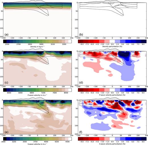
The vertical sections of the final FWI models along the CIFALPS transect are displayed in Figs 6(a), (c) and (e) for the V_P, V_S and ρ parameters. This representation is complemented by that of the model perturbations (computed with respect to the initial model) to highlight the resolution improvement achieved by FWI (Figs 6b, d and f). The model perturbations roughly remove the imprint of the low-wavenumber components from the FWI model and, hence, mimic the intermediate wavenumber components that could be imaged by the migration of receiver functions. We superimpose on these vertical sections the structural interpretation proposed by Zhao et al. (2015) to facilitate the identification of the main structural units (Fig. 6, black lines). The ρ, V_p and V_s models show similar structures with, however, their own resolution. As expected, the V_p model is less well resolved than that for V_s in accordance with the P and S wavelengths. In contrast, the ρ and V_s models show a similar high-wavenumber content in the upper part of the lithospheric target, which is consistent with the analysis of their radiation patterns (Fig. 2). However, the FWI clearly fails to significantly update ρ below 70 km depth, unlike V_s. As suggested in Section 2, this might result from the deficit of wavefield sensitivity to ρ perturbations in the forward-scattering regime. According to the teleseismic setting, this forward scattering is more suitable to update the deep part of the lithosphere. Since backscattered waves should undergo two reflections from the free surface and the lithospheric reflectors to sample the deep lithosphere, it is unlikely that such second-order scattered waves can be recorded with a sufficient signal-to-noise ratio for FWI.

Figure 6.

Open in new tabDownload slide

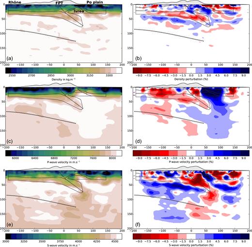
Vertical sections of the FWI models along the CIFALPS transect (W–E). (a–b) ρ. (c–d) V_p. (e–f) V_s. The absolute values of the parameters and the perturbations are shown in (a,c,e) and (b,d,f), respectively. Black lines denote units as defined by Zhao et al. (2015). Perturbation models are computed with respect to the initial model. The topography is shown with a vertical exaggeration for illustration purpose. The black dashed line shows the location of the European LAB. X-axis is centred on the location of the Frontal Penninic Thrust (FPT).

Of primary interest is the Moho discontinuity. Being a first order seismic discontinuity this boundary generally exhibits strong impedance gradients that are nicely depicted by receiver functions computations and migrations. Our models delineate clear but rather complex Moho geometries beneath the Alpine orogeny. On the western part, the European Moho dips from roughly 30 km in the Rhône valley to 50 km beneath the Frontal Penninic Thrust (FPT; see Fig. 6). Further east, its dip increases and the Moho reaches a depth of around 65 km (on V_p and ρ models) at the transition between the internal Alps and the Po plain underlining a high density/ fast velocity anomaly corresponding to mantle material within the crust (blue blob on V_p model). On the V_s model, the Moho can be followed at greater depths, down to approximately 80 km. At this depth, the Moho is interrupted by a slow velocity anomaly that spreads horizontally from 50 to roughly 100 km of distance. On the eastern side, the Moho transition is more difficult to follow and exhibits strong topographic variations. Nonetheless, absolute velocity variations (Figs 6c–e) suggest a 40–50 km deep Moho boundary beneath the Po plain. In between, the area corresponding to the Ivrea body gravity anomaly is well delineated by a high density/fast velocity anomaly. In particular, the top-eastern boundary of this anomaly matches well the shape of the Ivrea body in the interpretative model of Zhao et al. (2015) (Fig. 6b). However, its top-western boundary highlights a very different geometry with a pronounced sub-vertical orientation ( Fig. 6f). The horizontal extent of this feature is depicted at multiple depths in Fig. 7 by a characteristic North-South pattern.

Figure 7.

Open in new tabDownload slide

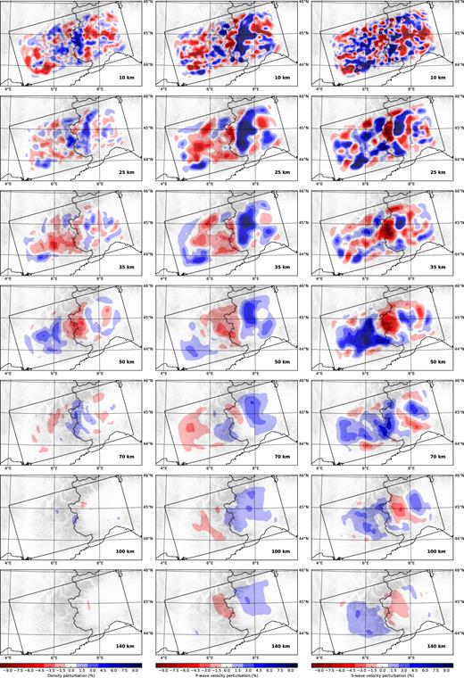
Depth slices of the FWI perturbation models. From left to right, ρ, V_p and V_s parameters. From top to bottom, slice at 10, 25, 35, 50, 70, 100 and 140 km depth. Perturbations are computed with respect to the initial model.

At shallower depth, from the surface to 20 km, the three models exhibit strong parameter perturbations. Caution must be taken examining these anomalies that are locally polluted by the acquisition footprint which takes the form of singularities at receiver locations. Nonetheless lateral structures can be followed that are consistent with the location and shape of sedimentary basins. Notably all parameters show strong negative perturbations—2000–2300 kg m⁻³, 5000–5500 m s⁻¹ and 2600–2800 m s⁻¹ for ρ, V_p and V_s, respectively—in the Po plain that correlates well with the basement of the sedimentary basins assumed to be 10 km thick. A similar behaviour is visible for the Rhône valley in the western part where slow P and S-wave (5500 m s⁻¹ and 3000 m s⁻¹) velocities are encountered.

At the upper-mantle scale, our models show small amplitude variations. Nonetheless, at depths ranging from 80 km to 120 km, we can follow the lateral continuity of a vertical transition corresponding to a decrease of the S-wave velocity. This transition may correspond to the lithosphere-asthenosphere boundary (LAB; Kissling & Spakman 1996; Eaton et al. 2009; Fischer et al. 2010). The depth of the LAB would thus vary from 80–90 km beneath the Rhône valley to 100–120 km at the transition between internal Alps and the Po plain. Interestingly, the structure of the upper mantle is sensibly different on the V_p and V_s models beneath the Ivrea zone. While a wide-spread high velocity anomaly characterizes the V_p model, a 50 km blob of low V_s is imaged just beneath the dipping European Moho. Laterally, this anomaly follows the arc of the Western Alps from 100 km to 140 km depth (Fig. 7).

3.4 Resolution and parameter cross-talk appraisal

Before discussing the geodynamical implications than can be drawn from the FWI models, it is worth appraising the ability of the teleseismic waveform inversion to resolve small-scale parameter perturbations by mean of resolution tests. Even though these resolution tests, which generally rely on local analysis around the minimum of the misfit function, cannot reveal whether the inversion has approached the global minimum of the misfit function (Lévěque et al. 1993; Fichtner & Trampert 2011; Trampert et al. 2013; Rawlinson & Spakman 2016), they still provide a cheap manner of assessing the resolution with which heterogeneities were reconstructed. As explained in section 2, FWI should be able to resolve anomalies whose sizes are of the order of the minimum propagated wavelength. At lithospheric scale, considering averaged V_p and V_s values of 7500 and 4000 m s⁻¹, and considering a minimal period of 5 s, we expect our FWI model to catch heterogeneities the sizes of which are of the order of 20 km. To verify this assumption and assess the spatial resolution of the FWI model, we designed a first resolution test by superimposing onto the final FWI model a coarse grid of 20 km-wide Gaussian (ρ, V_p, V_s) inclusions with positive and negative perturbations in alternates (±100 m s⁻¹ for V_p and V_s and ±100 kg m⁻³ for ρ). The spacing between the inclusions is sufficiently large and their amplitude sufficiently small to prevent a significant imprint of multiscattering (nonlinearity) during FWI.

We use the final FWI model as initial model of the resolution test such that this initial model reproduces all of the wave phenomena that occurred during the latter stage of the FWI, a necessary condition for a reliable resolution appraisal (Rawlinson & Spakman 2016). Synthetic data computed in the FWI model with the inclusions are then inverted following the same strategy as for the real data application with the final FWI model as initial model. The reconstructed inclusions are shown in Fig. 8. As expected from the teleseismic configuration, the ability of FWI to resolve parameter perturbations decreases with depth. While all of the three parameters are well-retrieved in amplitude and shape at 10 km depth, which is consistent with the theoretical resolution of FWI, FWI hardly recovers the true shape and amplitude of the anomalies at 70 km depth with horizontal and vertical smearing effects. This results from the combination of several factors. First, the increase of velocities with depth increases the local wavelengths and therefore decreases the resolution. Second, the inversions become increasingly ill-conditioned with depth due to incomplete correction for wave amplitude effects. This can make the imprint of deeply located scatterers in the wavefield too small to be exploited by the inversion. Third, the amount and strength of scattering might become more limited with depth as on the one hand the resolution of the FWI decreases and on the other hand the real heterogeneities of the deep lithosphere become milder and the free surface more distant. At 130 km depth, only the V_s parameter seems to be resolvable for 20 km-wide anomalies. This again might result on the one hand from the lack of penetration in depth of the ρ reconstruction and on the other hand to the longer wavelength of V_p relative to V_s.

Figure 8.

Open in new tabDownload slide

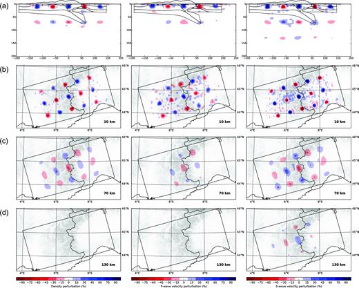
Resolution analysis. Reconstruction of fast and slow (ρ, V_p, V_s) Gaussian inclusions by multiparameter FWI (see the text for details). From left to right, ρ, V_p and V_s FWI perturbation models. (a) Vertical section along the CIFALPS transect. Depth slices at 10 km (b), 70 km (c) and 130 km (d) depth. The colour scale corresponds to the percentage of the true inclusion amplitude (100 m s⁻¹ for V_p and V_s and 100 kg m⁻³ for ρ.

It is also worth noting that, despite the 1-D nature of the receiver layout, our FWI model successfully recovers horizontal sections of the anomalies down to 70 km depth. Surprisingly, the depth slice at 10 km depth does not show significant aliasing artefacts in spite of the poor sampling of the receivers in the direction perpendicular to the CIFALPS transect (Figs 9b and c), although weak periodic patterns are visible in the S-wave perturbation model (Figs 9b and c). This good horizontal resolution may result from the joint contribution of the events with an oblique backazimuth with respect to the main CIFALPS transect and the off-line stations. The resulting source and receiver wave paths are favourable to record both forward and backward scatterings and enrich the horizontal wavenumber coverage in all part of the lithospheric model accordingly. A more thorough sensitivity analysis of teleseismic FWI to the station geometry is presented in Beller et al. (2018) and highlights the key contribution of off-line stations to improve both the vertical and horizontal resolution of the teleseismic imaging. To further assess how the resolution evolves with depth, we designed two additional resolution tests with only one 20 km wide fast (ρ, V_p, V_s) inclusion located at 50 and 100 km depth, respectively (Figs 9a and b). We use one inclusion per test to ensure that the reconstruction of this inclusion is not impacted upon by other close heterogeneities. The V_p FWI perturbation model shows significant vertical smearing supporting the fact that the vertical wavenumber components of this parameter are mainly reconstructed by forward scattering. In contrast, the ρ FWI perturbation model shows a horizontal smearing indicating a better vertical resolution relative to the horizontal one. This is consistent with the fact that the ρ reconstruction is mainly sensitive to back scattering generated by the double interaction of the wavefield with the free surface and the inclusion. This is well illustrated by the vertical alternates of positive and negative perturbations in the reconstruction at 100 km depth that highlights the deficit of low vertical wavenumbers in the ρ perturbation model.

Figure 9.

Open in new tabDownload slide

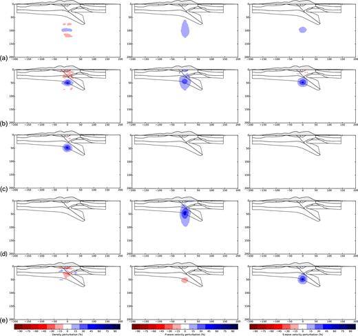
Resolution analysis and parameter cross-talk appraisal. From left to right, vertical section along the CIFALPS transect of the ρ, V_p and V_s FWI perturbation models. All of the panels show results of multiparameter FWI for ρ, V_p and V_s updates for either multiparameter (a,b) or mono-parameter (c–e) inclusion models (see the text for details). (a,b) Resolution analysis. Reconstruction of a fast 20 km wide (ρ, V_p, V_s) inclusion at 100 km (a) and 50 km (b) depths. (c–e) Parameter trade-off. (c) Reconstruction of a fast 20 km wide ρ inclusion at 50 km depth. (d) Same as (c) for a V_p inclusion. (e) Same as (c) for a V_s inclusion. Ghost of the inclusion in V_p and V_s models of (c), in ρ and V_s models of (d) and in ρ and V_p models of (e) highlight parameter cross-talk. The colour scale corresponds to the percentage of the true inclusion amplitude (100 m s⁻¹ for V_p and V_s and 100 kg m⁻³ for ρ).

In the framework of multiparameter reconstruction, it is crucial to assess to which extent the FWI models are affected by parameter cross-talk. We perform three multiparameter FWI by considering for each test a single-parameter inclusion involving V_P, V_S and ρ, respectively (Figs 9c–e). Any ghost of the inclusion in the reconstruction of a parameter that has no imprint in the data residuals will be the expression of the parameter cross-talk. The reconstruction of the ρ and V_p inclusions do not generate significant leakage in the models of the two other parameters (Figs 9c and d). In contrast, the reconstruction of the V_s inclusion generates some moderate leakage in the ρ and V_p perturbation models in the form of small negative perturbations. However, this leakage remains small, and prompts us to conclude that the (ρ, V_p, V_s) parametrization is reliable for teleseismic FWI.

A final resolution test is performed to check the reliability of the negative anomaly located at 100 km beneath the Ivrea zone in the V_s FWI model (Figs 6c and e). We add a 50 km-wide slow velocity/low density inclusion to the final V_p, V_s and ρ FWI models. The size of the inclusion was chosen according to that of the anomaly shown in the V_s FWI model of Figs 6(c) and (e). Results are presented in Fig. 10. Again, the shape of the anomaly is nicely recovered in the V_s FWI perturbation model, whereas the V_p reconstruction is affected by vertical smearing. For such large anomaly at rather great depth, FWI fails in recovering the true amplitude of the ρ perturbation, as expected. A partial conclusion is that the S-wave anomaly can be trusted while the P-wave one must be interpreted with caution in view of its intrinsic low vertical resolution.

Figure 10.

Open in new tabDownload slide

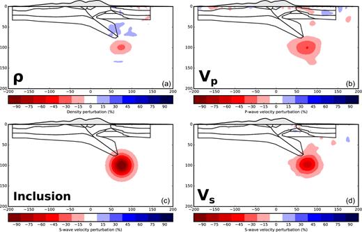
Resolution analysis for a 50 km-wide (ρ, V_p, V_s) inclusion located at the position of the negative V_s anomaly shown in Figs 6(c) and (e). FWI perturbation model for ρ (a), V_p (b) and V_s (d). The colour scale corresponds to the percentage of the true inclusion amplitude (c) (100 m s⁻¹ for V_p and V_s and 100 kg m⁻³ for ρ). The 50 km wide anomaly is a 3-D Gaussian located in the profile section at 100 km depth and x = 75 km.

4 DISCUSSION

4.1 Density parameter reconstruction

Through the analysis of scattering pattern in Section 2.3 and the recovery of sensitivity models in Section 3.4, we have seen that the joint use of amplitude and phase information contained in the waveform data enables the resolution of the density. The reconstruction of the density parameter is however restricted to the shallow part of the lithospheric model since it might require the recording of a doubly backscattered wavefield: reflected from the free surface and from a lithospheric heterogeneity. Moreover, as discussed in Section 3.2, density is sensitive to the noise content of the data. It is therefore relevant to examine the extent to which the update of V_p and V_s during FWI is sensitive to the way in which density is involved in the inversion, namely, as a passive parameter that is kept fixed over iteration as in Wang et al. (2016) or as an optimization parameter as in the current study. Fig. 11 presents the results of the FWI of CIFALPS data sets obtained by updating only V_p and V_s and by keeping ρ fixed to the initial smoothed PREM model. A quick comparison of these results with those of Fig. 6 indicates that the update of the ρ parameter does not significantly impact the reconstruction of the V_p and V_s parameters, that are very close to those obtained without involving the ρ parameter in the inversion. We conclude that accounting for ρ in teleseismic FWI does not degrade nor improve the recovery of kinematic parameters. Beyond that, it may allow for (shallow) inference on the density model through the use of the amplitude information. This statement is consistent with the conclusions of Prieux et al. (2013, their fig. 9) drawn from FWI applications on controlled-source seismic data. We thus believe it is worth updating the density to mitigate the effects of incorrect density information when no prior information on density is available (Plonka et al. 2016). This is supported by Yuan et al. (2015) who concluded that simultaneous update of ρ, V_p and V_s starting from an erroneous density model gives V_p and V_s models that are comparable to those we would obtain using the exact density information.

Figure 11.

Open in new tabDownload slide

Same as Fig. 6 except that the density model is kept fixed to the initial smoothed PREM model: only V_p and V_s are updated during FWI.

The relevance of the FWI ρ model of the Western Alps is further supported by the fair consistency between the measured and the computed regional Bouguer anomalies of the Alps, this latter being inferred from our FWI density model (Fig. 12). One measurement of the computed Bouguer anomaly map is obtained by integrating the attraction of all density perturbations within the FWI model with respect to the initial model. The Bouguer anomaly map of the Western Alps is dominated by negative anomalies that characterize the mass deficit generated by the thick crustal root of the Alps. These less dense crustal materials manifest in our density model as reddish negative anomalies as expected. This negative trend is flanked by a positive gravity anomaly associated with the north–south oriented Ivrea body, the shape of which (green lines on Fig. 12) is in good agreement with a high density anomaly at 25 km depth in our density model. Even though large-scale gravity features of the Western Alps are recovered, the Bouguer anomaly map computed from our FWI density model presents various small-scale features that do not correlate with real gravity measurements. These pollutions come from localized density perturbations at shallow depths (see Fig. 7). Apart from the loss of resolution, most of these perturbations are created by strong localized heterogeneities at receiver locations due to inherent singularities in the FWI sensitivity kernels.

Figure 12.

Open in new tabDownload slide

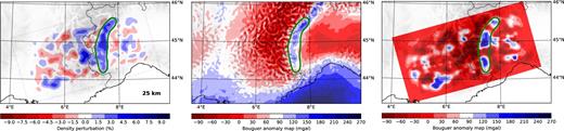
Comparison of the density perturbation model at 25 km depth, the regional Bouguer Anomaly map from Balmino et al. (2012) and the Bouguer anomaly map computed from our density perturbation model. The green line highlights the horizontal geometry of the Ivrea body.

4.2 Geodynamic interpretation

The Western Alps result from the convergence of Adriatic and European margins over the past 40 Ma and points to several subduction events since 100 Ma. Despite numerous geophysical studies, an integrated interpretation of surface observations, crustal and upper-mantle structures remains difficult because of complex 3-D structures and of the various sensitivities and resolutions of available imaging techniques that further complicate the understanding of the geodynamics evolution of the Alps. We believe that our FWI model provides a good compromise to fill the resolution gap between high-resolution images of the crust obtained from CSS, receiver functions and LET studies and lower resolution traveltime tomography images of the upper mantle.

For instance, our models of the Alpine lithosphere give a concise overview of the known Western Alps crustal structures. Notably, as seen in previous LET studies (Paul et al. 2001; Diehl et al. 2009), the structure of the upper crust is dominated by the high-velocity/high-density Ivrea body. This feature can be continuously traced down from 10 km to 50 km depth and appears to be connected to the Adriatic mantle as mentioned by Nicolas et al. (1990) and Schmid & Kissling (2000) who interpreted it as a mantle wedge indenter. The relatively high V_p (≈7400 m s⁻¹) together with a high V_p/V_s ratios clearly indicate the upper-mantle origin of this body. The shape of the ρ anomaly nicely follows the limits of the upper-crust model of Zhao et al. (2015). In agreement with Potin et al. (2015), the horizontal extent of the Ivrea body seems to be separated into two independent blocks: one to the north near Torino and the other one to the south near Cuneo (see V_p and particularly V_s at 25–35 km depth in Fig. 7). A striking feature of our V_P and V_S model concerns the western boundary of the Ivrea body anomaly. Contrary to the interpretative model of Zhao et al. (2015), our models highlight a sharp near vertical limit in the western part. This is consistent with the localization of seismicity within the Alpine crust as presented by Malusà et al. (2017) who showed that anomalously deep earthquakes are aligned on an active lithospheric fault located in the mantle wedge between the European and Adriatic Moho.

The question of the Moho geometry has long been an issue in the Western part of the Alps (Laubscher 1990; Marchant & Stampfli 1997; Lombardi et al. 2008; Spada et al. 2013). Evidences of continental subduction such as HP-LT coesites found by Chopin (1984) in the Dora Maira massif indicates continental crust burial at a depth of the order of 100 km. Neither LET nor teleseismic tomography studies had a sufficient resolution to precisely image this first order discontinuity of the crust that was finally imaged thanks to receiver function migration (Zhao et al. 2015) along the same CIFALPS transect. Our FWI model clearly delineates the Moho topography beneath the external and internal part of the Alps that is in good accordance with the results of Zhao et al. (2015). Our V_p and ρ models agree in following the European Moho discontinuity down to approximately 70 km depth while our (better resolved) V_s model tends to define a Moho boundary down to 80–90 km depth beneath the Ivrea body. Our models therefore support the assumption of subduction of the European continental lithosphere.

The subduction of continental lithosphere raises the question of the fate of continental and oceanic slabs. Early regional traveltime tomography studies of the Alpine region (Spakman et al. 1993; Bijwaard & Spakman 2000; Piromallo & Morelli 2003) have indicated the presence of continuous fast velocity slabs underlying the Alpine Belt down to 150 km depth. Underneath, the mantle transition zone also appears to be dominated by high-velocity materials. The fast anomalies have been interpreted as cold material that are remnants of subducted slabs. Recently, Lippitsch et al. (2003) built an image of the Western Alps upper mantle with an improved resolution by crustal-corrected traveltime inversion. Their investigation revealed striking complexities in the velocity structure of the uppermost mantle. They observed a detached fast anomaly from 150 to 300 km depth beneath the Western part of the Alps that is bordered in the West by a slow velocity anomaly. The upper part of their model – from 80 to 120 km depth – displays a two-block (separated at the location of the Ivrea body) fast velocity anomaly that may indicates the extent of the European and Adriatic LAB. These observations agree with our V_p and V_s FWI models that also identify a variation of LAB from 80 to 120 km depth. We particularly recover the anomalously slow velocities in the Western part of the Alps lithosphere that indicates a zone of anomalously high temperature therefore positively buoyant mantle that has previously been interpreted as asthenospheric upwelling (Lippitsch et al. 2003). Such asthenospheric flow has been interpreted by von Blanckenburg & Davies (1995) as a consequence of the oceanic slab detachment that may explain extensional earthquakes in the Western Alps as suggested by Sue et al. (1999). Moreover, Nocquet et al. (2016) recently proposed that present-day uplift rates in the Alps (that are several times larger than horizontal velocities) may result from upward traction at the base of the Alpine lithosphere. They propose that this uplift may thus be due to the replacement of dense mantle material by more buoyant one, therefore sustaining the idea of asthenospheric upwelling.

The block separation of the lithosphere beneath the Ivrea body is not visible in our V_p model that displays a continuous positive anomaly down to 150 km depth, nonetheless our V_s model indicates a blob of slow velocity at the same location. We remind that the V_s velocity model is better resolved than the V_p model, whose resolution might be hampered by strong vertical smearing at these depths. The wide positive anomaly in the V_p model might result both from the downward smearing of the fast Ivrea body and from the upward smearing of the detached slab that would be located just beneath the depth limit of our FWI model according to the tomographic model of Lippitsch et al. (2003). The negative V_s anomaly can either result from thermal effects or the presence of fluid. The fact that the negative V_s anomaly does not correlate with a V_P negative anomaly strongly supports the presence of fluid or melts at the base of the continental crust at the expense of the thermal effect. These fluids or melts could have been released from the subducted hydrated oceanic lithosphere located beneath and possibly indicate the location of the slab detachment at 100 km depth beneath the Ivrea body.

In summary, our FWI image of the Alpine lithosphere suggests the hypothesis of the slab detachment (or slab break-off) in the Western part of the Alpine Belt as proposed by von Blanckenburg & Davies (1995). The lithospheric structure of the whole Alpine Belt as imaged by Lippitsch et al. (2003) further indicates that the detachment is restricted to the Western part since in the Central Alps the European slab can continuously be traced within the lower-lithosphere suggesting a lateral migration of the slab detachment: the slab tear hypothesis (Wortel & Spakman 2000). Lippitsch et al. (2003) proposed that the slab break-off at the Ivrea location might be caused by the Ivrea body that could have acted as a buttress during the collision of European and Adriatic lithosphere, forcing the European slab to sink beneath the Adriatic lithosphere. Nonetheless, the question of slab break-off in the Western part of the Alpine range is still controversial. A very recent finite-frequency P-wave tomography of the Alps upper mantle is presented by Zhao et al. (2016a). Their image continuously traces down the European slab from 70 km down to 300 km depth ruling off the break-off hypothesis.

Even though we favour the slab break-off hypothesis to explain the negative anomaly of the V_S model, such interpretation does not give unambiguous argument for this mechanism. Particularly, the recovered absolute velocities of the V_S model can either be related to both mantle or crustal material. Other plausible interpretations would imply a deeper subduction of the European crust down with an accumulation of lower crustal material to approximately 100 km depth. Another possibility would be to interpret this anomaly as the signature of the fluid-induced serpentinized mantle resulting from the subduction the alpine ocean passive margin.

Further investigations with AlpArray and CIFALPS-2 data will help in improving the data coverage and hence the resolution of the seismic images at greater depths. FWI of the crust as well as the upper mantle down to 600 km depth might give new clues about the fate of the European slab.

5 CONCLUSIONS

We presented the results of a multiparameter 3-D elastic FWI of the CIFALPS teleseismic data set recorded in the Western Alps. We showed that FWI, by using the full information content of the seismograms, is able to generate multiparameter images of the lithosphere with unprecedented resolution. Particularly, we emphasized the ability of FWI to recover reliable density information on the upper lithosphere. Recovered images of the Western Alps lithosphere agree well with previous receiver function, LET and teleseismic tomography studies as well as regional gravity measurements. Our models nicely display sharp crustal structures of the Western-Alps, notably, the Ivrea body and the Moho boundary and support the idea of a continental subduction event during the Alpine orogeny. Additionally, the revealed structures of the lower lithosphere support the hypothesis of a slab detachment or slab tear in the Western Alps. We show that the application of FWI at lithospheric scale fills the resolution gap between highly resolved crustal structures provided by receiver function analysis and classical tomographic images of the upper mantle. Further applications may be considered for more complex elastic properties of the medium using the transverse component or even bigger time window to include first S-wave arrival and its multiples. Added constrains on density reconstructions may be provided if one consider a joint inversion with gravity data. The new data sets obtained from current AlpArray or future CIFALPS-2 experiments will provide additional lithospheric information on the Alpine Belt and may confirm current interpretations.

Acknowledgements

We warmly thank L. Combe for invaluable help in the code development, especially for designing the domain decomposition library that allowed high-performance parallelism, and J. Virieux who encouraged the use of the CIFALPS data set and motivated fruitful discussions. This study also benefits from discussions with E. Bozdağ, Y. Rolland, J.-X. Dessa and A. Sladen. The CIFALPS project is funded by the State Key Laboratory of Lithospheric Evolution, China, the National Natural Science Foundation of China (Grant 41625016) and by a grant from Labex OSUG@2020 (Investissements d’avenir - ANR10 LABX56, France). This study was partially funded by the SEISCOPE consortium (http://seiscope2.osug.fr), sponsored by BP, CGG, CHEVRON, EXXON-MOBIL, JGI, PETROBRAS, SAUDI ARAMCO, SCHLUMBERGER, SHELL, SINOPEC, STATOIL, TOTAL and WOODSIDE. This study was granted access to the HPC resources of SIGAMM infrastructure (http://crimson.oca.eu), hosted by Observatoire de la Côte d’Azur and which is supported by the Provence-Alpes Côte d’Azur region, and the HPC resources of CINES/IDRIS under the allocation 046091 made by GENCI.

REFERENCES

APPENDIX A: SOURCE WAVELET IMPLEMENTATION

One difficulty of teleseismic waveform modelling and inversion with hybrid methods is to deal with the source wavelet estimation.

We remind that the location of the teleseismic earthquake is located outside of the computational domain. The teleseismic source is therefore implemented by applying a time dependent boundary condition on the edges of the lithospheric target. Propagating the wavefield for a new source signature therefore requires to convolve the source wavelet correction δs(t) with the incident wavefield everywhere on the outer boundary of the lithospheric target, hence leading to high computational cost and preventing, for example, periodic re-estimation on the fly of the source signature over several iterations.

Other interesting alternatives consist in modifying the cost function to make it insensitive to the source wavelet (Choi & Alkhalifah 2011; Beller et al. 2015; Zhang et al. 2016).

Author notes