Protostellar spin-down: a planetary lift?

Bouvier, J.; Cébron, D.

doi:10.1093/mnras/stv1824

Abstract

When they first appear in the HR diagram, young stars rotate at a mere 10 per cent of their break-up velocity. They must have lost most of the angular momentum initially contained in the parental cloud, the so-called angular momentum problem. We investigate here a new mechanism by which large amounts of angular momentum might be shed from young stellar systems, thus yielding slowly rotating young stars. Assuming that planets promptly form in circumstellar discs and rapidly migrate close to the central star, we investigate how the tidal and magnetic interactions between the protostar, its close-in planet(s), and the inner circumstellar disc can efficiently remove angular momentum from the central object. We find that neither the tidal torque nor the variety of magnetic torques acting between the star and the embedded planet are able to counteract the spin-up torques due to accretion and contraction. Indeed, the former are orders of magnitude weaker than the latter beyond the corotation radius and are thus unable to prevent the young star from spinning up. We conclude that star–planet interaction in the early phases of stellar evolution does not appear as a viable alternative to magnetic star–disc coupling to understand the origin of the low angular momentum content of young stars.

accretion, accretion discs, MHD, planet–disc interactions, planet–star interactions, stars: formation, stars: rotation

1 INTRODUCTION

It has long been known that the Sun and its siblings are characterized by quite modest rotational velocities, of the order of a few km s⁻¹ at most (e.g. Kraft 1970). This stands in sharp contrast to more massive stars that exhibit much higher spin rates all over their evolution. Schatzman (1962) first theorized that magnetized winds from solar-type stars would carry away a significant amount of angular momentum, thus braking the stars quite efficiently. Hence, regardless of their initial velocity, stars with outer convective envelopes would end up as slow rotators on the main sequence. This expectation was later confirmed by Skumanich (1972) who showed that the rotational velocity of solar-type stars appeared to steadily decrease on the main sequence, following the well-known Ω ∝ t^−1/2 relationship.

Extrapolating this relationship back in time to the early pre-main sequence (PMS), young stars were thus expected to be fast rotators at birth. More generally, as gravity dominates the late stages of protostellar gravitational collapse, newly born stars were commonly thought to rotate close to break-up velocity. Surprisingly, the first measurements of spin rates for low-mass PMS stars, the so-called T Tauri stars (TTS), did not meet these expectations. In contrast, young stars were found to have only moderate rotational velocities, on average about 10 times that of the Sun's, i.e. a mere 10 per cent of their break-up velocity (Vogel & Kuhi 1981; Bouvier et al. 1986; Hartmann et al. 1986). More than 30 years later, this aspect of the so-called initial angular momentum problem remains very much vivid.

Several physical processes have been proposed to account for the slow rotation rates of young solar-type stars. They all rely on the magnetic interaction between the young star and its circumstellar disc. At least three classes of models can be identified: X-winds (Shu et al. 1994), accretion-powered stellar winds (Matt & Pudritz 2005), and magnetospheric ejections (Zanni & Ferreira 2013). All these models investigate how the angular momentum flux between the star and its surrounding is modified by the magnetospheric interaction with the inner accretion disc. A brief outline of these models and a discussion of their specific issues can be found in Bouvier et al. (2014). While a combination of processes may eventually provide strong enough braking torques on young stars to account for their low spin rates, none have definitely proved to be efficient enough.

We investigate here an alternative process to account for the low angular momentum content of young stars. Specifically, we explore the flux of angular momentum being exchanged within a system consisting of a magnetic young star surrounded by a close-in orbiting planet embedded in the inner circumstellar disc. We review tidal and magnetic interactions between the protostar and a close-in planet to estimate whether spin angular momentum can be transferred from the central star to the planet's orbital momentum and eventually from there to the disc by gravitational interaction, thus effectively spinning down the central star. Previous papers have extensively explored star–disc, star–planet, and planet–disc interactions, usually with the aim to investigate the orbital evolution of close-in planets (e.g. Laine, Lin & Dong 2008; Chang, Gu & Bodenheimer 2010; Chang, Bodenheimer & Gu 2012; Lai 2012; Laine & Lin 2012; Zhang & Penev 2014). We build here from these earlier studies to explore the star–planet–disc interaction in the specific framework of the initial angular momentum problem. Indeed, while addressing the issue of halting planet migration near young stars through magnetic torques, Fleck (2008) mentions that such interactions may be at least partly responsible for the slow rotation rates of PMS stars. We will show here that, for realistic sets of stellar and planetary parameters, magnetic as well as tidal torques seem actually unable to prevent PMS stellar spin-up.

In Section 2 we describe the general idea developed here, summarize the parameters of the system, and express the requirement for an effective protostellar spin-down. In Section 3 we summarize the accelerating torques acting on the central star, namely accretion and contraction, that tend to spin it up. In Section 4, we explore both tidal torques and magnetic torques acting between the young star and the inner planet and review their efficiency in removing angular momentum from the central object. We discuss the quantitative torque estimates and the limits of the model in Section 5, and highlight our conclusions in Section 6.

2 STAR–PLANET–INNER DISC INTERACTION: A GENERAL framework

The general idea that we develop here is to investigate whether a fraction of the spin angular momentum of the star can be transferred to the orbital angular momentum of a close-in planet, which in turn could lose its excess angular momentum to the disc through tidal interaction. In this way, the planet would act as a ‘lift’ carrying angular momentum from the central star to the outer disc (cf. Fig. 1). We aim here at computing an equilibrium solution that would fulfil this requirement, and hence prevent the star from spinning up as it accretes and contracts. Alternatively, a more dynamical view of this process can be thought of, where the planet migrates successively inwards and outwards several times just outside of the corotation radius, thus transferring over time a significant fraction of the star's angular momentum to the outer disc.

Figure 1.

Open in new tab Download slide

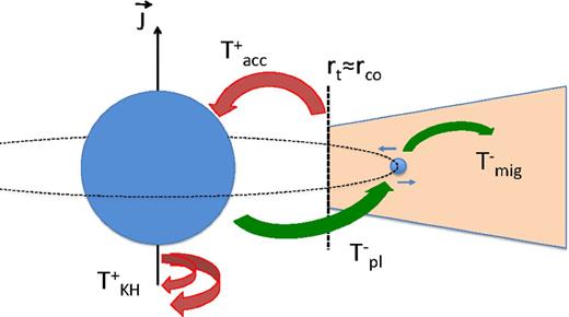
A sketch of the star–planet–inner disc interaction, with the main torques indicated: accretion, contraction, star to planet, planet to disc.

In the following subsections, we compute the torques acting in a system consisting of a young star, its circumstellar disc, and a close-in orbiting planet. The parameters of the system are listed in Table 1. To set orders of magnitude, we compute the specific angular momentum of the star, j_⋆, and of the planet, j_pl.

Table 1.

System parameters.

Star

M_⋆ = 1 M_⊙; R_⋆= 2 R_⊙; Ω_⋆= 5 Ω_⊙; B_⋆ = 1 kG

Disc/wind

|$\dot{M}_{\rm {acc}}$| = 10⁻⁹ M_⊙ yr⁻¹; |$\dot{M}^{\rm w}_\star$|= 10⁻¹⁰ M_⊙ yr⁻¹

Planet

M_pl = 10⁻³ M_⊙; R_pl = 0.2 R_⊙; τ_mig = 1 Myr

Open in new tab

The specific spin angular momentum of the central star is

\begin{equation} j_\star = {{J_\star }\over {M_\star }} = k^2 R_\star ^2 \Omega _\star , \end{equation}

(1)

with k² = 0.205 for a completely convective star, which yields j_⋆ = 5.8 × 10¹⁶ cm² s⁻¹. The specific orbital angular momentum of a non-eccentric planet orbiting at a distance a from the star is

\begin{equation} j_{\rm {pl}}= {{J_{\rm {pl}}}\over {M_{\rm {pl}}}} = (G M_\star a)^{1/2} \end{equation}

(2)

which is of the order of a few 10¹⁸ cm² s⁻¹ for an orbital semi-major axis of a few stellar radii. The specific angular momentum of the planetary orbit is two orders of magnitude larger than the specific angular momentum contained in the stellar spin. However, a Jupiter-mass planet orbiting at the corotation radius has nearly the same total angular momentum as the star,

\begin{equation} {{J_{\rm {pl}}}\over {J_\star }} = {{M_{\rm {pl}}(GM_\star a)^{1/2}}\over {k^2 M_\star R_\star ^2 \Omega _\star }} = {{M_{\rm {pl}}}\over {k^2M_\star }}\left({{\Omega _{{\rm br}}}\over {\Omega _\star }}\right)^{4/3} \simeq 0.2, \end{equation}

(3)

for |$a = r_{\rm {co}}= \Omega _\star ^{-2/3}(GM_\star )^{1/3}$|⁠, the break-up velocity |$\Omega _{{\rm br}}=(GM_\star )^{1/2}R_\star ^{-3/2}$|⁠, and the system parameters defined in Table 1.

3 SPIN-UP TORQUES: YOUNG STARS OUGHT TO ROTATE FAST

In this section, we describe torques that act to spin up young stars as they start their evolution on Hayashi tracks, namely the accretion and the contraction torques.

3.1 The accretion torque

A magnetic young star accreting from its circumstellar disc assumed to be in Keplerian rotation undergoes a spin-up torque expressed as

\begin{equation} T_{\rm {acc}}= \dot{M}_{\rm {acc}}r_{\rm t}^2 \Omega _{\rm {Kep}}(r_{\rm t}) = \dot{M}_{\rm {acc}}(G M_\star r_{\rm t})^{1/2}, \end{equation}

(4)

where |$\dot{M}_{\rm {acc}}$| is the mass accretion rate on to the star, r_t is the inner disc truncation radius, Ω_Kep is the Keplerian velocity in the disc, and M_⋆ is the stellar mass.

For the system parameters listed in Table 1, the stellar magnetosphere truncates the disc at a distance of

\begin{eqnarray} r_{\rm t}\approx 2B_\star ^{4/7} \dot{M}_{\rm {acc}}^{-2/7} M_\star ^{-1/7} R_\star ^{12/7} = 3.6\ 10^{11}\, \textrm {cm} = 5 \,\mathrm{R}_{\odot }= 2.5 R_\star ,\nonumber\\ \end{eqnarray}

(5)

where B_⋆ is the star's magnetic field and R_⋆ the stellar radius (Bessolaz et al. 2008).

Alternatively, assuming that the truncation radius is located close to the corotation radius in the disc

\begin{equation} r_{\rm t}\simeq r_{\rm {co}}= \Omega _\star ^{-2/3}(GM_\star )^{1/3} = 12\,\mathrm{R}_{\odot }= 6 R_\star , \end{equation}

(6)

where Ω_⋆ is the star's angular velocity.

For these values of the truncation radius, the accretion torque amounts to T_acc= 4.3–6.7 × 10³⁵ g cm² s⁻². The spin-up time-scale of the central star due to accretion is

\begin{equation} \tau ^{\rm {up}}_{\rm {acc}}= J_\star /T_{\rm {acc}}= {{k^2 M_\star R_\star ^2 \Omega _\star }\over {\dot{M}_{\rm {acc}}(GM_\star r_{\rm t})^{1/2}}}, \end{equation}

(7)

with the stellar angular momentum J_⋆ = 1.2 × 10⁵⁰ g cm² s⁻¹. Using the system parameters listed in Table 1, the spin-up time-scale thus amounts to 7 Myr and reduces to 0.7 Myr for a protostellar mass accretion rate of 10⁻⁸ M_⊙ yr⁻¹. Hence, as shown by Hartmann & Stauffer (1989), accretion from the circumstellar disc is expected to spin up the star to a significant fraction of its break-up velocity within a few Myr.

3.2 The contraction torque

As newly born stars descend their Hayashi track, their radius decreases and they eventually develop a radiative core. Both effects yield a reduction of the stellar moment of inertia and, if angular momentum is conserved, the star spins up. Taking into account only radius contraction during the first few Myr, the fully convective star can be described as a n = 3/2 polytrope.

The potential energy of a polytrope of index n is given by

\begin{equation} E_{{\rm pot}} = - {{3}\over {5-n}} {{GM_\star ^2}\over {R_\star }} \end{equation}

(8)

and the luminosity of a star undergoing homologous contraction is

\begin{equation} L_\star = - {{(3\gamma - 4)}\over {3(\gamma -1)}} {{{\rm d}E_{{\rm pot}}}\over {{\rm d}t}} = 4 \pi R_\star ^2 \sigma T_{{\rm eff}}^4. \end{equation}

(9)

The torque that should be applied to prevent the star from spinning up as it contracts down on the PMS on a Kelvin–Helmholtz time-scale is

\begin{equation} T_{\rm {KH}}= \Omega _\star {{\textrm {d}I}\over {\textrm {d}t}} = 2 k^2 M_\star \Omega _\star R_\star {{\textrm {d}R_\star }\over {\textrm {d}t}}, \end{equation}

(10)

and combining equations (8)–(10), with n = 3/2 and γ = 5/3, one finally gets

\begin{equation} T_{\rm {KH}}= {{14}\over {3}} k^2 {{\Omega _\star R_\star ^3}\over {GM_\star }} L_\star . \end{equation}

(11)

With the reference parameters listed in Table 1 and assuming T_eff = 4000 K, one finds T_KH ≃ 5 × 10³⁵ g cm² s⁻². Hence, stellar contraction is equivalent to an accelerating torque whose magnitude is similar to that of the accretion torque. Both contraction and accretion will thus equally act to spin the young star up.

4 SPIN-DOWN TORQUES: CAN THEY PREVENT FAST ROTATION?

In this section, we investigate the torque a planet orbiting outside the corotation radius would exert on to the central star. Such a planet would extract angular momentum from star and migrate outwards. At the same time, the planet feels the tidal torque from the disc through Lindblad resonances and tends to migrate inwards. An equilibrium configuration could result if the torques acting on the planet balance outside the corotation radius, thus ensuring a continuous transfer of angular momentum from the star to the planet and from the planet to the disc (cf. Fig. 1). If the outward net flux of angular momentum can counteract the accretion and contraction torques, the star will thus be prevented from spinning up. Whether such an equilibrium configuration can be reached, and whether it is able to effectively spin the star down, depends on the nature and strength of the star–planet–disc interaction. We first discuss tidal effects, and then turn to magnetic interactions.

4.1 Tidal torques

We investigate whether tidal torques are strong enough to allow the orbiting planet to extract spin angular momentum from the star and to pass it on to the outer disc. In order to spin the star down, the planet must be located beyond the corotation radius. The inward migration torque the disc-embedded planet experiences must therefore be balanced by the star–planet tidal torque beyond the corotation radius for the lift to operate.

The migration torque exerted by the disc on the planet can be expressed as

\begin{equation} T_{{\rm {disc}}}= {{\textrm {d}J_{\rm {pl}}}\over {\textrm {d}t}} = {1\over 2} M_{\rm {pl}}(GM_\star )^{1/2} a^{-1/2} {{\rm d}a\over {\rm d}t} \sim {J_{\rm {pl}}\over \tau _{\rm {mig}}}, \end{equation}

(12)

where τ_mig is the planet's migration time-scale in the inner disc.

We may first verify that the magnitude of the migration torque outside the corotation radius would be able to compensate for the accretion and contraction torques. The condition can be written as

\begin{equation} \left|T_{{\rm {disc}}}(a\ge r_{\rm {co}})\right| \ge \left|T_{\rm {acc}}+ T_{\rm {KH}}\right| \simeq 2\left|T_{\rm {acc}}\right|. \end{equation}

(13)

Using the above expressions for the accretion and migration torques, and assuming that the inner disc is located at the corotation radius (cf. equation 6), this translates to

\begin{equation} {a\over r_{\rm {co}}} \ge \left( 2 \tau _{\rm {mig}}{\dot{M}_{\rm {acc}}\over M_{\rm {pl}}}\right)^2 \end{equation}

(14)

which, adopting parameters from Table 1, yields a ≥ 4r_co. Hence, if a giant planet can be hold off beyond the corotation radius, it may effectively extract enough angular momentum so as to compensate for the accretion and contraction torques, thus preventing the central star from spinning up.

Is the tidal effect between the star and the planet strong enough to prevent the planet from migrating inwards of the corotation radius? The tidal torque is given by¹

\begin{equation} T_\star = {9\over 4} {M_{\rm {pl}}^2 \over \left(M_{\rm {pl}}+M_\star \right)} \Omega _{\rm {pl}}\left(\Omega _{\rm {pl}}- \Omega _\star \right) {R_\star ^5\over {Q_\star a^3}}, \end{equation}

(15)

where the migration rate of the planet due to the tidal interaction with the star is given by

\begin{equation} \left({\textrm {d}a\over \textrm {d}t}\right)_\star = \textrm {sign}(\Omega _\star - \Omega _{\rm {pl}}) {9\over 2} \left({G \over {aM_\star }}\right)^{1/2} \left({R_\star \over a}\right)^5 {M_{\rm {pl}}\over Q_\star } \end{equation}

(16)

with Ω_pl being the planet orbital rotation rate and Q_⋆ the tidal dissipation factor (e.g. Zhang & Penev 2014). The sign of the migration depends on whether the planet orbits within or beyond the corotation radius. The migration induced by the disc is always inwards

\begin{equation} \left({\textrm {d}a\over \textrm {d}t}\right)_{{\rm disc}} = -{a\over \tau _{\rm {mig}}}. \end{equation}

(17)

In order to slow the star down, the planet must orbit beyond the corotation radius. Hence, the planet's inward migration must be stopped before it reaches the corotation radius. We must then have

\begin{equation} \left({\textrm {d}a\over \textrm {d}t}\right)_\star \ge \left|\left({\textrm {d}a\over \textrm {d}t}\right)_{{\rm disc}}\right| \end{equation}

(18)

for r ≥ r_co all the way down to the corotation radius. Combining equations (16) and (17), we compute the critical semi-major axis at which the disc and stellar torques have the same amplitude on the planet (see also Lin, Bodenheimer & Richardson 1996),

\begin{equation} a_{\rm {crit}}= \left({{9M_{\rm {pl}}\tau _{\rm {mig}}}\over {2Q_\star }}\right)^{2/13}\left({G\over M_\star }\right)^{1/13}R_\star ^{10/13}. \end{equation}

(19)

At a semi-major axis larger than a_crit, the planet will migrate inwards, while for distance smaller than a_crit, the migration will be outwards. In order to ensure outward migration at or beyond the corotation radius, as required to brake the central star, a_crit must thus be larger than r_co. Using parameters listed in Table 1, and Q_⋆= 10⁶, one finds a_crit= 2.4 × 10¹¹ cm = 1.7R_⋆= 0.3r_co. The magnitude of the tidal torque thus appears unable to prevent the planet from migrating inwards the corotation radius, at which point it will contribute to spin up the star. Indeed, the tidal torque decreases very steeply with distance as seen from equation (16). Its amplitude at the corotation radius is about four orders of magnitude weaker than required to balance the migration and accretion torques (cf. Fig. 2), a result which is barely sensitive to the parameters of the system (cf. equation 19).

Figure 2.

Open in new tab Download slide

Magnitude of the torques (in accretion torque units). Considering the left vertical axis, the curves show the magnetic torque of the TE mode [equation (28) and R_obs = R_pl], of the Alfvén wings [equation (31) and R_obs = R_pl], the dipolar interaction [ϵ = 1, equation (25) for a dipolar planetary surface magnetic field of 10 G], the tidal torque, the magnetic torque associated with the unipolar inductor model [equation (32), with a planetary conductivity of σ_pl = 10⁻² S m⁻¹], and the migration torque (τ_mig = 10⁶ yr), shown by a dotted line. From left to right, the solid lines are, respectively, the corotation and the Alfvén radii, whereas the vertical dashed line shows r_v, the upper radius of the favourable DC circuit closure regime. We have also plotted, for comparison, the empirical formula obtained by Strugarek et al. (2014) from 2.5D numerical simulations. Note also the change of slope noticeable at a distance of 5R_⋆ in some curves, which is due to the SW becoming unable to prevent the magnetic planet to develop an extended magnetosphere. Only the magnitude of the torques is plotted, not their sign, which is the reason why the tidal torque (cf. equation 15) does not change sign at the corotation radius in this plot.

4.2 Magnetic torques

4.2.1 Models and kind of magnetic interactions

In this section, we aim at estimating orders of magnitude of the magnetic torques exerted by the planet on the star. To do so, we model the planet and the star as objects with a given radial profile of electrical conductivities, possibly generating magnetic fields. Naturally, this also models magnetic interactions between a moon and its planet, such as Io and Jupiter. The following is thus valid for star–planet or moon–planet magnetic interactions.

In the simplest case considered by some authors (Laine et al. 2008; Chang et al. 2010, 2012), vacuum is assumed between the star and the planet. If the star and the planet both generate a dipolar field, the magnetic torque is simply given by the cross-product of the magnetic moment with the magnetic field produced by the other dipole (which tends to align the magnetic moments). Torque can also come from dissipative effects. Typically, any time variation of the magnetic field in an electrically conductive domain will generate eddy currents, leading to Joule dissipation and torques. This is the so-called transverse electric (TE) mode (Laine et al. 2008), and the associated torques are e.g. studied by Chang et al. (2012) in the case of a planet orbiting in a tilted stellar magnetic field, which generates eddy currents in the conducting planet.

Actually, the space between the star and the planet is rather filled by an stellar winds (SW) originating from the star, which can be roughly modelled as an electrically conducting fluid in motion. This has, in particular, two consequences: (i) the stellar magnetic field is advected by the SW, which is the so-called interplanetary magnetic field (IMF), and decays thus less rapidly than in vacuum, and (ii) waves and currents can exist between the star and the planet allowing new kinds of magnetic interactions. The former point leads to a stronger TE mode in the planet, due to the higher time-varying magnetic field advected by the SW. The latter point requires one to investigate the interaction between the planet and the surrounding magnetized flow of the SW.

The star–planet interaction via the SW can be of various kinds, depending on the planet's velocity |$\boldsymbol {v}_{{\rm orb}}$| relative to the stellar wind (SW) local one |$\boldsymbol {v}_{{\rm sw}}$|⁠, the speed v_{A, f} of the fastest wave in the SW (i.e. the so-called fast magnetosonic wave), and the speed v_A of the shear (or intermediate) Alfvén wave. First, if the (fast) Alfvén Mach number |$M_{{\rm A,f}}=||\boldsymbol {v}_{{\rm orb}}-\boldsymbol {v}_{{\rm sw}}||/v_{{\rm A,f}}$| is larger than 1, the obstacle constituted by the planet generates a shock wave. In this so-called super-Alfvénic case, the flow is controlled upstream and disturbances are transmitted downstream. This is the case for Venus for instance, where the shock wave takes the usual form of a (detached) bow shock due to its bluff (i.e. non sharp-nosed) geometry. In the case where the planet generates its magnetic field, like the Earth, this changes the apparent radius of the obstacle (aka the magnetosphere radius) for the SW, leading to an enhanced coupling. This case of magnetic interaction between the SW and the planet is called magnetospheric interaction by Zarka (2007).

Secondly, we consider the sub-Alfvénic case (M_{A, f} < 1), focusing first on the simple case where the planet is weakly magnetized or unmagnetized. In this case, the planet motion generates shear (or intermediate) Alfvén waves which propagate in the SW and transport some energy from the planet to the star. The wave can then be reflected back, from the star to the planet, which leads to a planet–star interaction. Since the disturbance is only partially reflected, each subsequent reflection is of lower amplitude, and results in a lesser change to the current system (Crary & Bagenal 1997). After several round-trip travel times, the system reaches a steady state, and a current loop is settled. In this case, the star–planet interaction can be modelled as a DC circuit (Goldreich & Lynden-Bell 1969), which is called the unipolar inductor model or the TM mode (Laine 2013). In the other limiting case, the planet has moved away when the wave comes back and the planet's interaction is thus decoupled from the star. This is the so-called Alfvén wings (or Alfvénic interactions) model (e.g. Saur et al. 2004). These two models, sometimes presented as two different kinds of interaction, originate actually from the same phenomena and have been primarily applied to the Io–Jupiter interaction, but also to planets around magnetic dwarfs, ultracompact white dwarf binaries, exoplanetary systems, etc.

In the regime M_{A, f} < 1, we finally have the case where both the planet and the star generate a magnetic field. In the stellar system, the only example of such a case is the Ganymede–Jupiter interaction, which constitutes a textbook example of the expected plasma environment around close-in extrasolar planets (Saur 2014). This kind of interaction is often termed the dipolar interaction (e.g. Zarka 2007).

4.2.2 A generic torque formula

Focusing on dissipative torques, one can link the dissipated power P_d with the star–planet dissipative torque T by

\begin{equation} P_{\rm d}=T ||\boldsymbol {v}_{{\rm pl}}-\boldsymbol {v}^{B}||/a, \end{equation}

(20)

where a is the star–planet distance, |$\boldsymbol {v}_{{\rm pl}}$| is the planet velocity (v_pl ≈ Ω_pla), and |$\boldsymbol {v}^{B}$| is the advective velocity of the magnetic field at the planet orbit (i.e. the SW velocity |$\boldsymbol {v}^{B}=\boldsymbol {v}^{{\rm sw}}$|⁠, or v^B = Ω_⋆a in the absence of SW flow). Dimensional arguments allow one to write any torque exerted on the planet by the star as

\begin{equation} T=\epsilon \, a\, A_{{\rm eff}}\, P_{{\rm eff}}^{{\rm ram}}, \end{equation}

(21)

where ϵ is a dimensionless coefficient, a is the star–planet distance, A_eff is the typical surface area on which the star–planet magnetic coupling is effective, and |$P_{{\rm eff}}^{{\rm ram}}$| is the typical energy density of the coupling on the area A_eff (which can be seen as the ram pressure of the SW when an SW is considered). Focusing only on the magnetic coupling, this formula reduces to

\begin{equation} T=\epsilon \, a\, A_{{\rm eff}}\, \frac{B_{{\rm eff}}^2}{\mu _0} =\epsilon \, a\, \pi R_{{\rm obs}}^2\, \frac{B_{{\rm eff}}^2}{\mu _0}, \end{equation}

(22)

where B_eff is a typical magnetic field value exerted on the area A_eff, μ₀ is the magnetic permeability of the vacuum, and |$R_{{\rm obs}}=\sqrt{A_{{\rm eff}}/\pi }$| is the typical radius of A_eff.

Equation (22) requires the knowledge of ϵ, B_eff, and A_eff. The expression of ϵ depends on the magnetic interaction we consider, which is discussed in Section 4.2.3. The calculation of magnetic field B_eff depends on the medium between the planet and the star. If this is vacuum, then B_eff is simply deduced from the Gauss coefficients of the stellar magnetic field. If an SW exists, B_eff is simply given by the model chosen for the SW. Finally, A_eff depends on the planet. In the absence of any external conductive layer, R_obs = R_pl, which is thus a lower bound for R_obs. However, a planet has usually an ionosphere due to photoionization of the upper atmosphere (even without any own magnetic field), which leads to an induced magnetosphere above the ionosphere. This also means that the time-varying stellar magnetic field can be shielded by the ionosphere such that induced eddy currents in the planetary interior are small. Note that, as argued by Chang et al. (2012), atmosphere circulation may maintain this so-called exo-ionosphere on the permanent nightside of a tidally locked planet. In this case, the radius R_obs to consider is the exo-ionospheric radius, which is typically R_iono = 1.1–1.4 R_pl in the case of Io (Zarka 2007). Finally, the planet can also have its own magnetic field, either stored in its rocks or generated by dynamo. In this case, the planet develops its own magnetosphere. The magnetopause radius R_MP is then the apparent radius R_obs to consider, which can be estimated by the balance between the total ram pressure p_ram coming from the star and the planetary magnetic field B_pl:

\begin{equation} R_{{\rm MP}} = R_{\rm {pl}}\left[ \frac{B_{\rm {pl}}^2}{2\, \mu _0\, p_{{\rm ram}}} \right]^{\frac{1}{2m}}, \end{equation}

(23)

where m depends on the planetary magnetic field geometry (m = 3 for a mainly dipolar magnetic field, m = 4 for a mainly quadrupolar magnetic field, etc.), and where

\begin{equation} p_{{\rm ram}}=\frac{1}{2} \rho \, ||\boldsymbol {v}_{{\rm pl}}-\boldsymbol {v}^{{\rm sw}}||^2+\frac{1}{2} \frac{B_{{\rm eff}}^2}{\mu _0}. \end{equation}

(24)

Finally, R_obs is thus simply given by

\begin{equation} R_{{\rm obs}}=\max (R_{\rm {pl}},R_{{\rm iono}},R_{{\rm MP}}). \end{equation}

(25)

Particular forms of the generic formula (22) have already been considered in previous works. For instance, neglecting |$\boldsymbol {v}_{{\rm pl}}$| in equation (20) allows one to recover equation 9 of Zarka (2007), where B_eff = B_⊥ is the IMF component perpendicular to the SW flow in the planet's frame. Similarly, equation 9 of Chang et al. (2010) is recovered with equation (22), assuming no SW and a dipolar stellar field, such that B_eff = B_⋆(R_⋆/a)³, and considering |$R_{{\rm obs}}=\sqrt{2}\, R_{\rm {pl}}$|⁠.

As stated by Zarka (2007), this general expression is simply the fraction ϵ of the magnetic energy flux convected on the obstacle (aka the planet), and is expected to provide a correct order of magnitude whatever the interaction regime (unipolar or dipolar, super- or sub-Alfvénic) as long as the obstacle conductivity is not vanishingly small. The physics of the interaction is now hidden in the coefficient ϵ, which is the difficult estimate we have to obtain.

4.2.3 Application of the formula

In this work, we aim at studying if the star can be slowed down by planetary magnetic torque. Since the super-Alfvénic regime only allows disturbances to be transmitted downstream, this requires us to consider the sub-Alfvénic regime such that a torque can be exerted by the planet on the star. Given that the SW accelerates when flowing away from the star, this imposes to consider orbital distance a smaller than the so-called Alfvén radius given by (Bessolaz et al. 2008)

\begin{equation} r_{\rm A}= \left({{B_\star ^4R_\star ^{12}}\over {2GM_\star \dot{M}_{\rm {acc}}^2}}\right)^{1/7} = 12R_\star , \end{equation}

(26)

distance at which the SW flow becomes super-Alfvénic.² We have thus to estimate torques in four cases: the TE mode, the Alfvén wings model, the dipolar interaction, and the unipolar inductor model.

Torque due to the TE mode: in this case, the torque is associated with the Joule dissipation in the interior of the planet, originating from the stellar magnetic field oscillating at the rate ω. Owing to the diffusive nature of the problem, one can thus estimate the Ohmic dissipation by (Campbell 1997, 1983; Laine et al. 2008; Chang et al. 2012)

\begin{equation} P_{{\rm ohmic}}=\mathcal {V}\, \omega \ \frac{B_{{\rm eff}}^2}{2 \mu _0}, \end{equation}

(27)

where |$\mathcal {V}$| is the volume where eddy currents take place. This is thus typically a thin shell of thickness δ, which gives |$\mathcal {V}=A_{{\rm eff}}\, \delta$|⁠, i.e. |$\mathcal {V} \approx 4 \pi R_{\rm {pl}}^2 \delta$| if it takes place at the surface of an electrically conductive planet. Noting η the typical planetary electrical diffusivity, δ = (2η/ω) is then the skin depth for our magnetic induction problem.

Finally, considering that ω ∼ Ω_pl, an upper bound of the torque is obtained for |$\mathcal {V}=4 \pi /3 R_{\rm {pl}}^3$|⁠, and we will thus use equation (22) using R_obs = R_pl and

\begin{equation} \epsilon =\frac{2}{3} \frac{R_{\rm {pl}}}{a}. \end{equation}

(28)

Alfvén wings: as shown by Drell, Foley & Ruderman (1965), the radiation of two pure linear Alfvén wings leads (when converted to SI units) to a torque given by formula (22), with the coefficient (see also Lai 2012)

\begin{equation} \epsilon =2\, M_{\rm A}, \end{equation}

(29)

where |$M_{{\rm A}}=||\boldsymbol {v}_{{\rm orb}}-\boldsymbol {v}_{{\rm sw}}||/v_{{\rm A}}$| is the shear (or intermediate) Alfvén wave Mach number, with |$v_{\rm A}=B^2/\sqrt{\rho \mu _0}$| being the shear (or intermediate) Alfvén wave velocity and ρ the SW density. The factor 2 in equation (29) naturally comes from the existence of two Alfvén wings. The work of Drell et al. (1965) has then been extended by Neubauer (1980) to the fully non-linear sub-Alfvénic situation, also including flow |$\boldsymbol {v}_{{\rm orb}}-\boldsymbol {v}_{{\rm sw}}$| which is not perpendicular to the background field |$\boldsymbol {B}$|⁠. Following Zarka (2007), and taking into account the existence of two wings, this leads to the extended formula

\begin{equation} \epsilon =\frac{2\, M_{\rm A}}{||M_{\rm A}\, {\hat{\boldsymbol {v}}_{\rm rel}}+ \hat{\boldsymbol {B}} ||}, \end{equation}

(30)

with the two unit vectors |${\hat{\boldsymbol {v}}_{\rm rel}}$| and |$\hat{\boldsymbol {B}}$|⁠, directing, respectively, the relative velocity |$\boldsymbol {v}_{{\rm orb}}-\boldsymbol {v}_{{\rm sw}}$| and the (background) magnetic field |$\boldsymbol {B}$|⁠. Note that we naturally recover equation (29) for M_A ≪ 1. Focusing on orders of magnitude, the factor 2 can be dropped, and the case where the flow is perpendicular to the magnetic field (⁠|${\hat{\boldsymbol {v}}_{\rm rel}} \cdot \hat{\boldsymbol {B}} =0$|⁠) leads then to (Zarka 2007)

\begin{equation} \epsilon =\frac{1}{\sqrt{1+1/{M_{\rm A}}^{2}}}, \end{equation}

(31)

for the Alfvén wings interaction. Note that, in this case, R_obs is of the order of R_obs ∼ R_pl, even in the presence of an exo-ionosphere. Note also that Alfvén waves cannot be radiated when r > r_A, and the Alfvén wings interaction is thus only valid for r < r_A.

Dipolar or magnetospheric interaction: as argued by Zarka (2007), the torques associated with these interactions can also be modelled by formula (22), using ϵ = 0.1–1 (typically, ϵ ≈ 0.3 in the sub-Alfvénic Ganymede–Jupiter interaction). Note that ϵ = 1 is in agreement with equation (31), which gives ϵ ∼ 1 for M_A ≥ 1. The important feature of this kind of interaction is the presence of a planetary magnetic field, which can lead to large magnetic interactions (due to large R_obs).

Unipolar inductor model (DC circuit or TM mode): in this case, first studied by Goldreich & Lynden-Bell (1969), the Alfvén waves’ round trips between the star and the planet allow one to reach a steady state, which can be modelled as a DC circuit. In the planetary frame, the electrical field |$\boldsymbol {E}=\boldsymbol {v} \times \boldsymbol {B}$| generated by the planetary velocity |$\boldsymbol {v}$| indeed allows one to close a DC circuit through the surrounding electrically conductive medium. An electrical current is thus flowing through the electrical resistances of the planet, |$\mathcal {R}_{\rm p}$|⁠, of the stellar footprint of the planet, |$\mathcal {R}_\star$|⁠, and of the two flux tubes crossing the SW, |$2 \mathcal {R}_{\rm f}$|⁠.

The difficult estimation of the three electrical resistances is performed here by following Laine & Lin (2012) and Laine (2013), who neglect |$\mathcal {R}_{\rm f} \ll \mathcal {R}_{\rm p},\, \mathcal {R}_\star$|⁠. According to the formula obtained by Laine & Lin (2012) and Laine (2013), we thus end up with

\begin{equation} \epsilon =\frac{8\ \mu _0\, a\, |\Omega _{\rm {pl}}-\Omega _\star | }{\pi \, (\mathcal {R}_{\rm p}+\mathcal {R}_\star )}. \end{equation}

(32)

One can distinguish different regimes of closures of the DC circuit (Laine 2013). In the so-called favourable DC circuit closure regime, the Alfvén waves have the time to perform the round-trip planet–star–planet, which actually imposes here that the planet is on an orbit below a certain distance r_v. In our model, r_v ≃ 8R_⋆. Analytical estimates of r_v are derived in Appendix A.

Note that the DC circuit is naturally opened for r > r_A. Note also that there is an upper limit to the magnetic interaction torque generated using the unipolar inductor model (Lai 2012). Indeed, when the circuit resistance is too small, the large current flow severely twists the magnetic flux tube connecting the two binary components, leading to the breakdown of the circuit. According to Lai (2012), this breakdown appears when

\begin{equation} \zeta =\frac{4\, \mu _0}{\pi } \frac{ a|\Omega _{\rm {pl}}-\Omega _\star |}{ \mathcal {R}_{\rm p}+\mathcal {R}_\star }=\frac{\epsilon }{2} \ge 1, \end{equation}

(33)

which limits ϵ to ϵ = 2 (corresponding to ζ = 1 in Lai 2012).

4.2.4 Results

In order to calculate the various torque estimates given above, an SW model is required. In this work, we have considered two SW models. One is adapted from Zarka (2007), as detailed in Appendix B, and the other one is described in Lovelace et al. (2008). Both give similar results as far as magnetic torques are concerned (cf. Appendix B). Using the SW model adapted from Zarka (2007), the results are summarized in Fig. 2, and compared with the tidal torque. Note that the magnetic torque associated with the DC circuit depends on the chosen planetary conductivity. It turns out that above σ_pl = 10⁻⁵ S m⁻¹ (as used in Fig. 2), the resistance is very small (ζ ≥ 1), and the torque is thus maximum, given by ϵ = 2.

Fig. 2 clearly illustrates the main result of this study. None of the planet-induced torques acting on the central star, be it tidal or magnetic, is able to balance the accretion torque beyond the corotation radius. Hence, at least with the parameters adopted here, the star–planet interaction cannot prevent the spin-up of the central star as it accretes from its circumstellar disc and contracts down its Hayashi track. Indeed, even the most powerful torques, corresponding to the dipolar interaction and the unipolar inductor model, fail by several orders of magnitude to match the magnitude of the migration torque beyond the corotation radius. We have also compared these results to Strugarek et al. (2014) 2.5D numerical simulations and found that their parametric torque formulation predicts order-of-magnitude torques similar to the DC and dipolar cases investigated here (see Appendix C for a short account of their parametric torque formulation).

One may wonder why the magnetic coupling seems to be efficient enough in the similar study of Fleck (2008), in contrast to our results. This is partly due to the fact that he prescribes the cross-sectional area A_eff of the magnetic flux tube linking a planet to its host star to be in the range α = 1–10 per cent of the stellar surface. Here, we determine A_eff self-consistently and show that it is of order of magnitude of |$\pi R_{{\rm obs}}^2$|⁠, where R_obs ≈ R_pl when the planet is close from the star, and thus |$\alpha \approx \pi R_{\rm {pl}}^2/4\pi R_\star ^2 \approx 0.2$| per cent with our values. Also, Fleck (2008) assumed a stronger magnetic field (2 kG) and a larger stellar radius (3 R_⊙) than we adopted here, which results in a much stronger torque (cf. his equation 14). Indeed, a 3 kG field associated with a 4 R_⊙ protostar would be required to obtain a torque comparable to the accretion and migration torques.

5 DISCUSSION

We have considered the various torques acting in a system consisting of a contracting PMS star still accreting from its circumstellar disc into which a newly formed Jupiter-mass planet is embedded on a short-period orbit. We have shown that a balance between accelerating torques acting on to the star, due to accretion and contraction, and decelerating ones, due to the star–planet interaction, cannot be reached under the conditions we explored here. For all cases we investigated, the accretion torque exceeds any planetary torque acting on the central star by orders of magnitude.

The main limitation of the scenario outlined here lies in the adopted wind model. The model is an extrapolation from solar-type wind properties, which is not necessarily adapted to the wind topology of young stars. First, the topology of the magnetic field of young stars might be quite different from that of mature solar-type stars (e.g. Donati & Landstreet 2009), although current measurements suggest that fully convective PMS stars at the start of their Hayashi tracks host strong dipolar fields, of the order of a few kG (Gregory et al. 2012; Johnstone et al. 2014). Secondly, as shown by Zanni & Ferreira (2009), the structure of the stellar magnetosphere might be significantly impacted by its interaction with the circumstellar disc. In particular, an initially dipolar magnetic field may evolve into a much more complex and dynamical topology. Whether this would significantly modify the torques associated with the magnetic star–planet interaction is yet unclear.

Another issue of course is whether the framework proposed here is applicable to the vast majority of young stars that rotate slowly as they appear in the HR diagram. This would require that planet formation be not only a common occurrence, but also that it is fast enough to impact the earliest stages of stellar evolution, and that it is quite dynamic so as to frequently send massive planets on inner orbits. Whether all these conditions are met around protostars is yet unknown. The recent ALMA image of the numerous gaps in the disc of the protostar HL Tau suggests that multiple planet formation may indeed proceed quite rapidly after protostellar collapse. The significant fraction of hot Jupiters (HJs) found to revolve around their host star on a non-coplanar orbit further suggests that dynamical interaction between forming planets in the protostellar disc may be efficient to scatter massive planets close to their parent star (Fabrycky & Tremaine 2007; Triaud et al. 2010; Morton & Johnson 2011; Albrecht et al. 2012; Crida & Batygin 2014). Eventually, HJs are deemed to coalesce with the central star after a few hundred million years (Levrard, Winisdoerffer & Chabrier 2009; Bolmont et al. 2012). Hence, the scarcity of HJs around mature solar-type stars does not necessarily exclude that they are much more common during early stellar evolution (e.g. Teitler & Königl 2014; Mulders, Pascucci & Apai 2015).

Finally, we wish to emphasize that the preliminary results presented here have to be extended in order to explore a much larger parameter space. Table 1 summarizes typical parameters for young accreting stars that we adopted here for the torque computations. However, classical TTS at a given mass and age exhibit a wide range of spin rates (Bouvier et al. 2014), mass accretion rates (Venuti et al. 2014), magnetic field strength, and topology (Donati et al. 2013). Hence, the torque estimates provided here may vary significantly from one system to the next. Moreover, during the embedded phase, other sets of parameters could be relevant, implying for instance a larger radius, and possibly stronger magnetic fields (e.g. Grosso et al. 1997; Tsuboi et al. 2000) and faster rotation rates (e.g. Covey et al. 2005). Whether the planetary lift scenario could be instrumental in the protostellar embedded phase to produce the low angular momentum content of revealed young stars remains to be ascertained. Also, more complex scenarios than that described here could be envisioned. For instance, the planetary migration torque could be significantly reduced, and the migration time-scale considerably lengthened, by tidal resonances occurring between several inner planets embedded in the disc, or by considering a steeper surface density profile in the disc close to the magnetospheric cavity. In the latter case, the enhanced outward flux of angular momentum between the inner disc material and the close-in planet would result in sub-Keplerian disc rotation close to the truncation radius, thus potentially reducing the accretion torque on to the central star.

6 CONCLUSION

As an alternative, or a complement, to star–disc interaction models that attempt to account for the low spin rates of newly born stars, we explored here the tidal and magnetic interactions between a young magnetic star and a proto-HJ embedded in the inner disc. We investigated whether such a close-in embedded planet could extract enough angular momentum from the central star to counteract both the accretion and contraction torques, thus leaving the star at constant angular velocity as it evolves on its Hayashi track. While a lot remains to be done in exploring the parameter space relevant to such systems, it appears that the decelerating torques acting on the central star are orders of magnitude too weak to counterbalance the spin-up torques. Hence, even though planetary systems may promptly form around embedded young stars, as suggested by the recent ALMA image of HL Tau's disc³, star–planet interaction may not eventually prove a viable alternative to magnetic star–disc interaction to understand the origin of the low angular momentum content of young stellar objects.

We warmly thank Caroline Terquem for her input regarding tidal interactions and for a critical reading of a first version of the manuscript. It is a pleasure to acknowledge a number of enlightening discussions with P. Zarka, S. Brun, A. Strugarek, S. Matt, A. Vidotto, C. Zanni, and J. Ferreira on the complex issue of star–planet–disc-wind magnetic interactions. We would like to dedicate this short contribution to the memory of Jean-Paul Zahn, a pioneer in the development of the theory of stellar tides, who passed away a week before this paper was accepted.

1

The factor of 2 difference between equation (15) above and equation 18 of Chang et al. (2010) arises from their use of the apsidal motion constant which amounts to half the tidal Love number used to estimate the tidal quality factor Q_⋆ (cf. Mardling & Lin 2002).

2

Using the expression of the Alfvén radius from Matt & Pudritz (2008)'s SW models (their equation 14) would result in twice as large an estimate.

3

cf. http://www.eso.org/public/unitedkingdom/news/eso1436/

REFERENCES

Albrecht

S.

et al.

ApJ

2012

757

18

Month:	Total Views:
December 2016	1
January 2017	1
March 2017	2
May 2017	4
June 2017	1
July 2017	2
August 2017	4
November 2017	1
January 2018	2
February 2018	1
April 2018	1
May 2018	3
June 2018	2
August 2018	2
November 2018	1
December 2018	7
January 2019	2
February 2019	7
March 2019	8
April 2019	10
May 2019	19
June 2019	6
July 2019	12
August 2019	3
September 2019	10
October 2019	12
November 2019	10
December 2019	4
January 2020	7
February 2020	9
March 2020	5
May 2020	2
June 2020	6
July 2020	3
August 2020	7
September 2020	6
October 2020	3
November 2020	4
December 2020	2
January 2021	8

Article Contents

Protostellar spin-down: a planetary lift?

Abstract

1 INTRODUCTION

2 STAR–PLANET–INNER DISC INTERACTION: A GENERAL framework

3 SPIN-UP TORQUES: YOUNG STARS OUGHT TO ROTATE FAST

3.1 The accretion torque

3.2 The contraction torque

4 SPIN-DOWN TORQUES: CAN THEY PREVENT FAST ROTATION?

4.1 Tidal torques

4.2 Magnetic torques

4.2.1 Models and kind of magnetic interactions

4.2.2 A generic torque formula

4.2.3 Application of the formula

4.2.4 Results

5 DISCUSSION

6 CONCLUSION

REFERENCES

APPENDIX A: ANALYTICAL ESTIMATES OF rv FOR THE UNIPOLAR INDUCTOR MODEL

APPENDIX B: SW MODEL ADAPTED FROM ZARKA (2007)

APPENDIX C: RESULTS OF STRUGAREK ET AL. (2014)

Citations

Views

Altmetric

Email alerts

Astrophysics Data System

Citing articles via

Latest

Most Read

Most Cited

This Feature Is Available To Subscribers Only

APPENDIX A: ANALYTICAL ESTIMATES OF r_v FOR THE UNIPOLAR INDUCTOR MODEL