


Abstract
The seismoelectric method is based on the interpretation of the electrical field associated with the conversion of mechanical to electromagnetic energy during the propagation of seismic waves in heterogeneous porous media. We propose an extension of a poroacoustic model that takes into account fluid flow and the effect of saturation. This model is coupled with an electrokinetic model accounting for the effect of saturation and in agreement with available experimental data in sands and carbonate rocks. We also developed new scaling laws for the permeability, the streaming potential coupling coefficient and the capillary entry pressure of porous media. The theory is developed for frequencies much below the critical frequency at which inertial effects starts to dominate in the Navier–Stokes equation (>10 kHz). The equations used to compute the propagation of the P waves and the seismoelectric effect in unsaturated condition are solved with finite elements using triangular meshing. We demonstrate the usefulness of a recently developed technique, seismoelectric beamforming, to localize saturation fronts by focusing seismic waves and looking at the resulting seismoelectric conversions. This method is applied to a cross-hole problem showing how a saturation front characterized by a drop in the electrical conductivity and compressibility is responsible for seismoelectric conversions. These conversions can be used, in turn, to determine the position of the front over time.
1 INTRODUCTION
The seismoelectric method has recently received a lot of attention because of its sensitivity to heterogeneities in mechanical, hydraulic and electrical properties (e.g. Hunt & Worthington 2000; Fourie 2003; Zhu et al. 2008; Jardani et al. 2010) and the detection of resonance effects in porous formations (see Revil & Jardani 2010 for heavy oils and Jougnot et al.2013 for the presence of fractures). Since Pride (1994), most of the modelling efforts in computing the seismoelectric effect (e.g. Pride & Haartsen 1996; Haartsen & Pride 1997; Garambois & Dietrich 2002; Haines 2004; Hu et al.2007) have been based on the following assumptions: (1) use of a Biot theory (Biot 1956a,b) in solving the equations for the solid and fluid displacements vectors, (2) solving the electromagnetic problem in the diffusive limit of the Maxwell equations and (3) using an electrokinetic theory based on the use of the zeta potential (a local electrostatic potential defined inside the electrical double layer coating the surface of the solid phase).
Revil, Jardani, and coworkers (Jardani et al.2010; Revil & Jardani 2010; Araji et al.2012; Revil & Mahardika 2013) have recently developed an alternative approach based on (1) solving the Biot theory in terms of the solid displacement vector and the fluid pressure (a classical approach in mechanics, e.g. Karpfinger et al. 2009, but curiously not used in the modelling of seismoelectric effects), (2) solving the electromagnetic problem in its quasi-static limit of the Maxwell equations and (3) used an electrokinetic theory based on the charge per unit pore volume as an alternative to the zeta-potential-based model. The advantages of this modelling approach are (1) the speed of the forward modelling is increased considerably because we are solving the hydromechanical equations for four unknowns in 3-D (six unknowns in the approach used by Pride and followers). (2) The speed of the electromagnetic forward problem is also drastically increased (solving a Poisson-type equation is indeed much faster than solving a diffusion-based problem and reasonably accurate for the seismoelectric problem). (3) The model based on the volumetric charge density is using additional relationships between the charge density and the permeability, decreasing the total number of unknowns in the petrophysical model. This allows, as shown below, a straightforward extension of the theory at partial saturations. The gain taken in the computational speed of the forward problem has been used to implement different inversion algorithms based on complementary stochastic (Jardani et al.2010) and deterministic (Araji et al.2012) methods. Recently, Sava & Revil (2012) have proposed to use a poroacoustic approximation to speed up the computation of the seismoelectric problem for very complex geometries.
With the exception of Revil & Mahardika (2013) and Warden et al. (2013), all the seismoelectric theories (Pride 1994; Revil & Jardani 2010) have been developed in fully water-saturated conditions. The goal of this paper is to propose a simple yet accurate poroacoustic theory coupled with dynamic electrokinetic theory for partially saturated porous media. Unsaturated streaming potentials have also recently attracted some attention in looking at vadose zone transport properties (Mboh et al. 2012) and CO2 sequestration (Vieira et al.2012; Talebian et al.2013).
We consider below a porous material (isotropic) with two immiscible pore fluids, air (or oil) and water, water being the wetting phase. The non-wetting phase is considered to be a good insulator. We neglect the electrical double layer associated with the air (oil)/water interface (Leroy et al.2012) assuming that the surface area associated with this interface is much smaller than the charge density contribution associated with the minerals/water interface. The extension of the seismoelectric theory to unsaturated conditions is actually quite straightforward. It will be based on a combination of a simple, poroacoustic theory to which we added an extension of the electrokinetic theory in unsaturated conditions (Linde et al.2007; Revil et al.2007).
2 THEORY
2.1 Poroacoustic theory in saturated conditions
Because the curl of a gradient is always equal to zero, we have the property ∇ × u(r, t) = 0. The displacement is irrotational, which means that the pressure wave is purely longitudinal and corresponds to a P wave with a seismic velocity given by eq. (16).
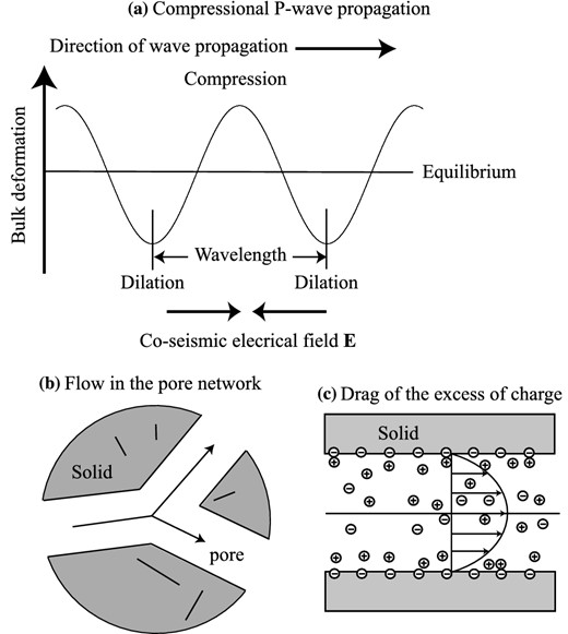
The coseismic electrical field and the coseismic (streaming) electrical current. (a) The propagation of a compressional (pressure or P) wave through a porous material generates areas of compression and dilation (expansion). (b) In response to the change in the mechanical stresses, the pore water flows from the compressed regions to the dilated regions. (c) The flow generates a streaming current density that is locally counterbalanced by the conduction current density creating, locally, an electrical field E of electrokinetic nature.
In summary, the properties entering the poroacoustic approximation used above are the undrained bulk modulus Ku, the drained modulus of the skeleton K, the bulk modulus of the pore fluid Kf, the shear modulus G (which is equal to the shear modulus of the skeleton), the permeability at saturation kS and finally the dynamic viscosity of the pore fluid ηf. In unsaturated conditions, we will need to expand these properties as a function of saturation.
2.2 Dynamic electrokinetic theory at saturation
Solving eqs (23) and (24) is required to understand the electrical disturbance associated with the passage of a seismic wave through a heterogeneity, such as an interface (Fig. 2). In this case, the electrical field is called the seismoelectric conversion.
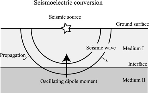
The seismoelectric conversion (called sometimes the interface response) results from the generation of an unbalanced source current density at an interface during the passage of a seismic wave. The divergence of the source current density at the interface is mathematically similar to an oscillating dipole moment generated at the interface in the first Fresnel zone. The star represents the position of the seismic source.
In summary, the properties entering the electrical problem are the effective charge density |$\hat Q_V$|, the formation factor F and the surface conductivity corresponding to the last term of eq. (25). These three parameters will be explicitly related to the saturation in the next sections.
2.3 Influence of saturation
This equation has been recently challenged by Jougnot et al. (2012) but seems however to be consistent with experimental data as checked by Linde et al. (2007), Revil et al. (2007) and Mboh et al. (2012). We will show later that this model is also consistent with the data from Guichet et al. (2003), Revil et al. (2011) and Vinogradov & Jackson (2011).
3 ADDITIONAL SCALING RELATIONSHIPS
3.1 Relative permeability
In this section, we developed a unified set of scaling relationship between the hydraulic and electrical properties in order to reduce the number of input parameters. Three scaling laws are developed below, one for the relative water permeability, one for the capillary entry pressure and one for the streaming potential coupling coefficient. For each new scaling law, we will show that it is in agreement with existing experimental data or empirical scaling laws based on fitting experimental data.
This result is very important because it provides an explicit relationship between a hydraulic parameter and an electrical parameter. To our knowledge, this is the first time that these relationships are proposed despite some attempts to connect the resistivity index and the capillary pressure curves (see for instance Li & Horne 2005).
In Fig. 3, we have plotted a number of experimental data from the literature in terms of the Brooks and Corey exponent versus the saturation exponent. Note that both in the case of the data of Maerefat & Chang (1987) and those of Jun-Zhi & Lile (1990), we plotted the corresponding saturation exponent as functions of the Brooks and Corey parameter taken from Brooks & Corey (1964) for the Shannon and Berea sandstones both characterized by a narrow porosity range. Fig. 3 shows that Model A seems to agree better than Model B with experimental data but more data are needed to check the predictive capabilities of the two models. These new relationships also mean that the measurement of the second Archie's exponent can be used to predict the capillary pressure curve and hysteretic behaviour in the capillary pressure curve should imply a hysteretic behaviour in the value of n.
3.2 Capillary entry pressure
This equation can be compared to the empirical equation derived by Thomas et al. (1968), |$p_e = 52k_S ^{ - 0.43} ,$| with pe expressed in kPa and kS in mD. Archie's law F = ϕ− m can be used to compute F from the porosity and the cementation exponent. Taking m = 2.0 (a default value for sandstones, see Revil et al.1998, their fig. 5) and a porosity ϕ = 0.20 (a reasonable average value), we obtain |$p_e = a\,k_S ^{ - 0.5}$| with a = 61 with pe expressed in kPa and kS in mD. We also obtain |$p_e = b\phi /\sqrt {k_S }$|. The proportionality between the capillary entry pressure and the ratio |$\phi /\sqrt {k_S }$| is checked in Fig. 4. Therefore, eq. (53) is able to represent data but accounts explicitly for the porosity dependence, which is not the case of the empirical equation developed by Thomas et al. (1968).
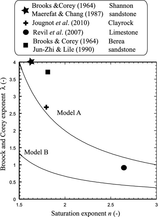
Comparison between Models A and B used to predict the value of the Books and Corey exponent l from the saturation exponent. Data from Jougnot et al. (2010), Revil et al. (2007), Brooks & Corey (1964), Maerefat & Chang (1987) (value extrapolated at ambient pressure and 25 ºC) and Jun-Zhi & Lile (1990). The Shannon sandstone is also known under the term ‘Hygiene sandstone’ in the literature. For the Berea sandstone, the data of Maerefat & Chang (1987; their fig. 3) yield a very similar value than those of Jun-Zhi & Lile (1990) when extrapolated at 25 ºC and ambient pressure. The data seem to favour Model A over Model B but more data are needed to test the models.
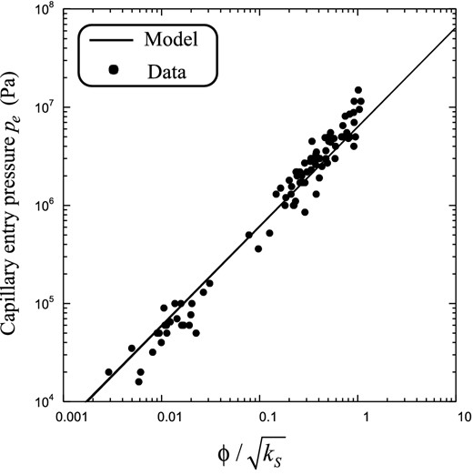
Comparison between the model proposed in the main text for the capillary entry pressure assuming that the formation factor is related to the porosity by F = ϕ− 2 (classical Archie's law, Archie 1942). The experimental data are from Huet et al. (2005). They correspond to 89 sets of mercury-injection (Hg–air) capillary pressure data. Core samples include both carbonate and sandstone lithologies. The permeability is expressed in mD.
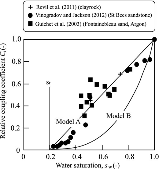
Comparison between Models A and B to predict the value of the relative streaming potential coupling coefficient as a function of the water saturation. We use an irreducible water saturation sr = 0.2. Data from Revil et al. (2011), Vinogradov & Jackson (2011) and Guichet et al. (2003). The data seem to favour Model A over Model B.
3.3 Relative coupling coefficient with the Brooks and Corey model
In Fig. 5, we compare the two models to the existing data replacing the water saturation by the irreducible saturation to satisfy to the additional constrain that there is no flow at the irreducible water saturation. Very clearly, Model B is unable to explain these data.
3.4 Relative coupling coefficient with the Van Genuchten model
Mboh et al. (2012) measured the relative streaming potential coupling coefficient of a clean silica sand characterized by the following properties: 99.3 per cent silica, porosity ϕ = 0.41, hydraulic conductivity K = 8.25 × 10⁻⁵ m s−1, mean grain diameter d = 160 μm (Table 1). Their data are exceptionally good in terms of quality. It is indeed difficult to get very good data in unsaturated conditions because of the drift of the electrodes (see discussions in Revil & Linde 2011 and Jougnot & Linde 2013 for the drift associated with saturation effects and Petiau & Dupis 1980 and Petiau 2000, for other sources of noises). Their column was equipped with 10 non-polarizable Ag/AgCl electrodes and six T5 tensiometers and the acquisition were done at 1 kHz.
| Property | Symbol | M | E3 | E39 |
|---|---|---|---|---|
| Saturation exponent | n (–) | 1.87 | 2.7 | 3.5 |
| Cementation exponent | m (–) | – | 1.93 | 2.49 |
| Permeability | k (m2) | 8.4 × 10⁻¹² | 48.4 × 10⁻¹⁵ | 23.8 × 10⁻¹⁵ |
| Porosity | ϕ (–) | 0.41 | 0.203 | 0.159 |
| Residual saturation | sr (–) | 0.09 | 0.31 | 0.34 |
| Grain size | d (μm) | 160 | – | – |
| Pore size | r (μm) | – | 1.18 | 0.17 |
Mboh et al. (2012) measured a coupling coefficient at saturation of C = –3.3 mV m−1 for a pore water conductivity (tap water) of σw = 0.044 S m−1 at 25ºC. The second Archie exponent (Saturation exponent) was measured and found to be equal to n = 1.87. The Van Genuchten exponent was measured and was found to be equal to nv = 3.88 (by fitting the capillary pressure curve). This yields mv = 0.74. A comparison between the data of Mboh et al. (2012) and eq. (62) is shown in Fig. 6. The best fit of the data yields mv = 0.69 ± 0.05; therefore, very close to the value determined from the capillary pressure curve (Fig. 6). As mentioned by Mboh et al. (2012), this implies that the values of the relative coupling coefficient bears information regarding the Van Genuchten parameters as suggested by Linde et al. (2007) and Revil et al. (2007).
In Figs 7 and 8, we reanalysed the data presented in Revil & Cerepi (2004) and Revil et al. (2007) correcting few mistakes in the unit conversions found in these two papers. We analysed the streaming potential coupling coefficient data of samples E3 and E39 (dolomitic limestones, see properties in Table 1). In both cases, the second Archie exponent (saturation exponent) was independently determined using resistivity measurements. The Van Genuchten parameters were found to be roughly the same using the capillary pressure curves and the relative streaming potential coupling coefficient data.
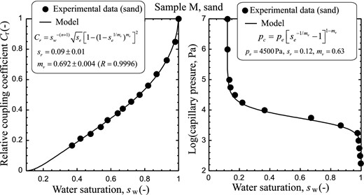
Comparison between experimental data and the prediction of the model developed by Revil et al. (2007) with the Van Genuchten model (see also Linde et al.2007). The experimental data are from Mboh et al. (2012) (sample M, sand). Left panel: Relative streaming potential coupling coefficient versus saturation. We used the measured value of the saturation exponent (second Archie exponent) n = 1.87. Right panel: Capillary pressure curve (non-wetting fluid: air).
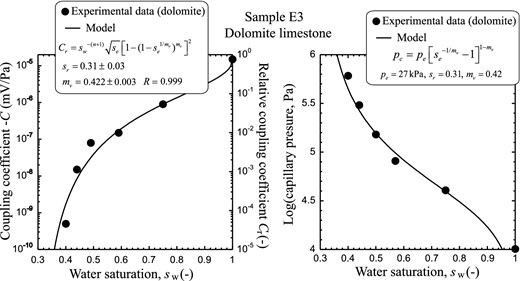
Comparison between experimental data and the prediction of the model developed by Revil et al. (2007) with the Van Genuchten model (see also Linde et al.2007). The experimental data are from Revil & Cerepi (2004) and Revil et al. (2007) (sample E3). Left panel: Absolute and relative streaming potential coupling coefficient versus saturation. We used the measured value of the saturation exponent (second Archie exponent) n = 2.7. Right panel: Fit of the capillary pressure curve with the same Van Genuchten parameters than obtained for the coupling coefficient (non-wetting fluid: mercury).
4 SEISMOELECTRIC BEAMFORMING IN THE POROACOUSTIC APPROXIMATION
4.1 Motivation
We apply here the seismoelectric beamforming approach developed recently by Sava & Revil (2012) to localize a discontinuity in resistivity associated with a water saturation front. We consider a 2-D case where we modelled a background porous material with constant mechanical, hydraulic and electrical properties. Two rectangular heterogeneities (Anomalies 1 and 2) are embedded in this background as shown in Fig. 9. The background and the two anomalies share the same mechanical properties and only their hydraulic and electrical properties differ from one to another because of a change in saturation (the material properties are reported in Table 2). The background is supposed to be fully water saturated (electrical conductivity of 1 S m−1) while the anomalies are more resistive (10−2 S m−1 for Anomaly 1 and 10−3 S m−1 for Anomaly 2 corresponding to two distinct saturations).
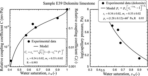
Comparison between experimental data and the prediction of the model developed by Revil et al. (2007) with the Van Genuchten model (see also Linde et al.2007). The experimental data are from Revil & Cerepi (2004) and Revil et al. (2007) (sample E39). Left panel: Absolute and relative streaming potential coupling coefficient versus saturation. We used the measured value of the saturation exponent (second Archie exponent) n = 3.5. Right panel: Fit of the capillary pressure curve with the same Van Genuchten parameters than obtained for the coupling coefficient (non-wetting fluid: mercury).
Petrophysical properties for the background and Anomalies 1 and 2.
| Property | Background | Anomaly 1 | Anomaly 2 |
|---|---|---|---|
| Undrained bulk modulus Ku (Pa) | 22 × 109 | 22 × 109 | 22 × 109 |
| P-wave velocity Vp (m s−1) | 3093 | 3093 | 3093 |
| Excess charge density |$\hat Q_V$| (C m−3) | 0.20 | 2.0 | 6.7 |
| Log (permeability, k in m2) | –12 | –14 | –16 |
| Skempton coefficient B | 0.65 | 0.65 | 0.65 |
| Average density ρ (kg m−3) | 2300 | 2300 | 2300 |
| Hydraulic viscosity of pore fluid ηf (Pa s) | 10−3 | 10−3 | 10−3 |
| Conductivity σ (S m−1) | 1 | 0.01 | 0.001 |
| Saturation sw (–) | 1 | 0.10 | 0.03 |
Seismic sources are located in two boreholes. The seismic sources (virtual geophones, seismic sources and electrodes) are set-up every 5 m along the ground surface and in the two wells (see Fig. 9, 19 sources in each well and 8 sources along the ground surface). Our objective is to beamform seismic waves at two specific points (positions A and B, see Fig. 9) and see if a seismoelectric conversion can be recorded by electrodes located in the wells in presence of a saturation front. When the seismic energy focuses on a heterogeneity, such as an interface, we expect to record a seismoelectric conversion (interface response). If we scan various points, this technique enables us to identify whether the point of focus is located close to a saturation front or not. The numerical experiment described below uses the acoustic approximation discussed in Section 2 above. We solved the partial differential equations for the mechanical and electrical problems in the frequency domain.
4.2 Beamforming technique
The beamforming technique enables us to focus seismic energy at a desired location and at a known time knowing approximately the velocity model. As discussed in Sava & Revil (2012), the velocity model does not need to be perfectly known. The seismic beamforming is done in two steps:
Step 1: On a finite-element grid, we choose the point of focus and we insert a fictitious seismic point source at this location. The seismic source is a Ricker wavelet with a dominant frequency of 500 Hz (Fig. 10). It contains energy up to about 1500 Hz. Using a constant seismic P-wave velocity of 3100 m s−1, we obtain a dominant wavelength of 6.2 m and a minimum wavelength of 2 m. That gives us a seismic resolution of 1.55 and 0.51 m, respectively. All numerical modellings were performed using the finite element package Comsol Multiphysics 4.3b using triangular meshing of non-constant element size (minimum element size of 0.0024 m and maximum element size of 1.2 m). This choice was driven by the need to have five elements of mesh per wavelength. In order to model the study areas without any seismic reflection at the boundaries (infinite medium), we used the CPML (convoluted perfect matched layer) developed by Jardani et al. (2010). The thickness of the CPML is 10 m around the area of interest. The seismic P waves are propagated from the source to fictitious electrodes located in place of the true seismic sources in the wells and along the ground surface. For one shot, we record the macroscopic pressure field Pi(t) at each geophone i located in the wells.
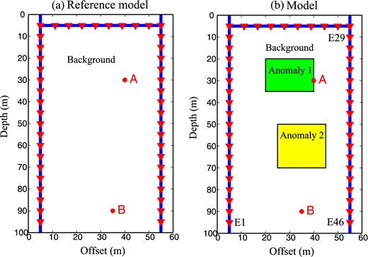
Geometry used for the beamforming problem. The medium consists of a homogeneous background model (reference model, fully saturated) plus two anomalies termed Anomaly 1 and Anomaly 2. These anomalies correspond to areas that are unsaturated (see Table 2). The survey area is surrounded by two vertical wells located on each side. The red triangles correspond to the location of the seismic sources/geophones/electrodes. The spacing between two consecutive sensors is 5 m. The two boreholes have 19 seismic set of sensors each and 8 additional set of sensors are located close to the ground surface (5 m deep). The two red-filled circles correspond to the focusing points used for our numerical experiments. Ei corresponds to the position of electrode i. They are 46 set of sensors in total with E1 and E46 are at the bottom of the two wells.
Step 2: Once the pressure fields have been recorded at each geophone, we back propagate the pressure fields as shown in Fig. 11. We first flip the signal recorded at each geophone (Pshifted(t) = Precorded(T – t), where T is the total recording time or listening time). We then create seismic point sources located at the position of the virtual geophones and we reinject the flipped seismic signals into the medium. Those flipped outgoing pressure fields will then propagate and interfere constructively at the original location (where we first put the seismic source, see Fig. 11). During this back propagation, we record the electrical potential at the wells and along the ground surface at the 46 electrodes colocated with the seismic source.
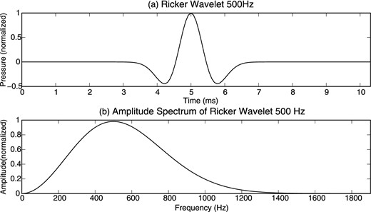
Pressure source f(r, t) (see eqs 12 and 13) used for the beamforming experiment. The pressure source is a Ricker wavelet with a 500 Hz dominant frequency and a time-shift of 5 ms. (a) Pressure time-series of the source. (b) Amplitude spectrum of the source.
The strength of this technique comes from the fact that we know exactly at what time and what location the seismic wavefields will focus and interfere constructively. If the point of focus is located on an interface, we will record an interface response with a greater amplitude that we would have recorded if there was only one wavefield crossing the interface. In fact, the electric potential diffused by a seismoelectric conversion due to a discontinuity in the medium properties is usually orders of magnitude smaller than the coseismic field (electrical field giving rise to an electrical 13 potential only detectable inside the support of a seismic wave). An example is shown in Fig. 11(f) showing the dipolar field created by the beamforming of the seismic waves at point A. This technique forces the interface response conversion to increase in amplitude due to the focusing of the different pressure fields coming from the multiple seismic sources.
By applying this technique to a grid of points within the survey area (by scanning the area point by point), we can then use the electrical response to map the discontinuities in terms of electrical and hydraulic properties of the material. We can also adjust and increase the resolution of our mapping by scanning over a denser grid of points around certain areas.
4.3 Results and interpretations
We focus seismic energy on few points of interests and we record the potential with 46 electrodes (19 in each borehole and 8 along the ground surface). The first point of focus (point A, see Figs 9 and 11) is located at an interface with a sharp discontinuity in conductivity and permeability. Therefore, we expect to see a seismoelectric conversion. Our results confirmed this assumption (Fig. 12). However, we need to remove the distribution of potential recorded with only the background to see the seismoelectric conversion associated with the interface response. We can clearly see that the dominant spike in the electric potential time-series (background removed) is perfectly synchronized with the focusing time of the seismic wavefield at point A. This enables us to detect a heterogeneity at point A.
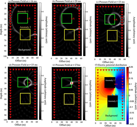
Seismic beamforming and resulting electrical potential distribution. (a)–(e). Snapshots showing the pressure field (coming from the 46 seismic sources shown in Fig. 9) focusing at point A. At t = 27 ms, the wavefield interfere constructively in point A and a strong seismoelectric is recorded at the receiver electrodes. (f) The distribution of the electrical potential (arbitrary units) corresponds to the case where the seismic energy is focused at point A. The seismoelectric conversion at the time of focusing is characterized by a strong dipolar behaviour.
Fig. 13 shows the electric potential at an electrode located at electrode E45 when the seismic wave are focused at point B, which is not located close to an interface. As expected, we see no spike at the focus time, which indicates a lack of heterogeneity at the focus point. Therefore, this method can be used in time lapse to follow the evolution of a saturation front over time, for example, for CO2 sequestration or to monitor water flooding experiments.
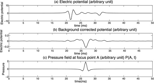
Beamforming at point A. (a) Time-series of the electrical potential at electrode E35 for beamforming the seismic wave at point A. The time-series comprise both the seismoelectric conversions and the coseismic field. The interface response is not detectable. (b) Electrical potential recorded when the medium contains the two anomalies minus the potential recorded if we only had the background. The interface response is now clearly visible. (c) Time-series of the pressure field at point B, P(A, t).
5 APPLICATION TO WATER FLOODING
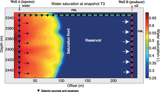
In this section, we apply the approach taken in Section 4 to a more realistic scenario. A lot of work has been done recently in using low-frequency electrical signals to detect oil–water encroachment fronts (see, for instance, Saunders et al.2008). We want to see if seismoelectric beamforming can be used to localize in a very simple way the position of the front. We consider two wells crossing a heterogeneous reservoir (see Fig. 14). Well B is located 250 m away from Well A and the total geometry of the model covers an area of 410 × 250 m. The reference position, O(0,0), is located at the upper-left corner of this domain. The reservoir is initially saturated with oil (oil saturation of 80 per cent). During water flooding operations, water is injected in Well A and oil is produced in Well B.
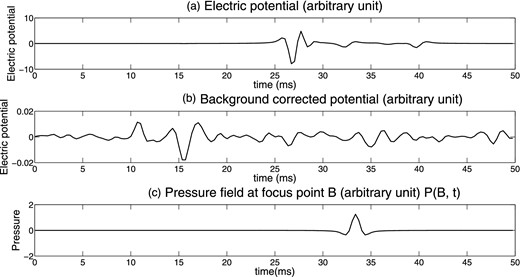
Beamforming at point B. (a) Time-series of the electrical potential at electrode E45. The time-series show both the seismoelectric conversions and the coseismic field. The interface response is not detectable. (b) Difference of two time-series: the electric potential in the top graph minus the electric potential recorded at the same location but for a homogeneous background (reference model). There is no conversion, which is consistent with the fact that point B is not associated with a heterogeneity. (c) Time-series of the pressure field at point B, P(B, t).
We use a random simulator to create a stochastic realization for the clay content and we use the model of Revil & Cathles (1999) to determine the porosity and the permeability at saturation. The multiphase flow simulator allows computing the saturation profiles, which are used to compute the P-wave velocity and resistivity distributions. The P-wave velocity and the permeability of the water phase are shown in Fig. 15 for snapshot 3, while the electrical conductivity and the porosity are shown in Fig. 16. The P-wave velocity does not depend too much on the saturation and its distribution is comprised between 4050 and 4300 m s−1. The electrical conductivity distribution varies over an order of magnitude. The influence of the water saturation is much greater on the resistivity than on the P-wave velocity.
Sketch of the domain used for the modelling. The total modelling domain is a 410 m × 250 m rectangle. Injector Well A is used, located at position x = 0 m, is also used for the seismic source. Production and recording Well B is located at x = 250 m. The discretization of the domain comprises a finite element mesh of 205 × 125 rectangular cells. A total of 28 receivers are located in Well B, approximately 30 m away from the nearest PML boundary (the PML boundary layers are shown in grey).
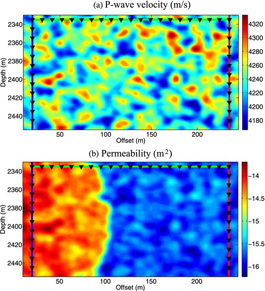
Sketch of the distribution of the P-wave velocity and permeability of the pore water phase at snapshop 3. Note that the saturation front is characterized by a sharp contract in permeability.
The seismic source is a Ricker wavelet (magnitude 1.0 × 10⁴ N m, delay time ts = 30 ms, dominant frequency fc = 160 Hz). We solve the poroacoustic equations described in Section 2 and the Poisson equation for the electrical potential in the frequency domain. The material properties are described in Table 3. In summary, we compute the properties distributions given the porosity, fluid permeability and saturation distributions, then we solve for the confining pressure P(r, t) of the solid phase and the pore fluid pressure p(r, t). Finally, we compute the electrical potential by solving the Poisson equation coupled to the poroacoustic problem for the frequency range 8–800 Hz. This range is valid for our problem since the seismic wave and the associated electrical field operates in the same frequency range. We then compute the inverse Fourier transform (FFT−1) to get the time-series of the seismic displacements ux and uz, and the time-series of the electric potential response.
Material properties used in the saturation front detection. We use Model A with m = n = 2.
| Parameter | Value | Units |
|---|---|---|
| ρs | 2650 | kg m−3 |
| ρw | 1000 | kg m−3 |
| ρo | 900 | kg m−3 |
| Ks | 36.5 | GPa |
| K | 18.2 | GPa |
| G | 13.8 | GPa |
| Kw | 2.25 | GPa |
| Ko | 1.50 | GPa |
| ηw | 1 × 10⁻³ | Pa s |
| ηo | 50 × 10−3 | Pa s |
| Parameter | Value | Units |
|---|---|---|
| ρs | 2650 | kg m−3 |
| ρw | 1000 | kg m−3 |
| ρo | 900 | kg m−3 |
| Ks | 36.5 | GPa |
| K | 18.2 | GPa |
| G | 13.8 | GPa |
| Kw | 2.25 | GPa |
| Ko | 1.50 | GPa |
| ηw | 1 × 10⁻³ | Pa s |
| ηo | 50 × 10−3 | Pa s |
The mesh is made of cell 2 × 2 m. The size of the mesh is smaller than the smallest wavelength of the seismic wave. For this mesh size, we check that the solution of the partial differential equations governing the seismoelectric problem is mesh independent. At the four external boundaries of the domain, we apply a 50-m-thick CPML.
Fig. 17 shows a pure transmission experiment between a seismic source located in Well A and an electrical receiver located in Well B. We also record the fluid pressure at the first Fresnel zone of the seismic wave at the position of the saturation front. Fig. 17 shows the existence of a strong seismoelectric conversion at the saturation front. This confirms the results of Revil & Mahardika (2013), who used a poroelastic theory.
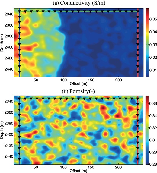
Sketch of the distribution of the electrical conductivity and porosity at snapshop 3. Note that the saturation front is characterized by a sharp contract in electrical conductivity.
Encouraged by this result, we apply now the seismoelectric beamforming discussed in Section 4 to this case. Figs 18(a)–(e) show the seismic beamforming using the seismic sources located in three wells. Fig. 18(f) shows the resulting electrical potential distribution at the time for which the seismic energy is beamformed. This shows a very strong dipolar field associated with the beamforming.
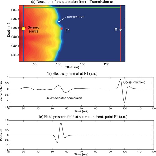
Transmission experiment with the seismic source in Well A and the electrical receiver in Well B. (a) Geometry of the test. (b) Time-series for the electrical potential showing the seismoelectric conversion occurring at the interface (like in Fig. 2) and the coseismic field (like in Fig. 1). (c) Fluid pressure field at a point located at the saturation front at the centre of the Fresnel zone.
In Fig. 19, we repeat this operation for a set of scanning pints located at the same depth and crossing the position of the saturation front. Our analysis shows that the strongest seismoelectric conversion is located at the position of the saturation front. Therefore, we can conclude that the scanning of the reservoir could be used to determine the position of the saturation front and to monitor its progression over time. An application of the present theory to a vadose zone case study is also developed in a companion paper (Kulessa et al. 2013).
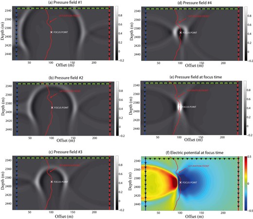
Seismic beamforming at the saturation front and resulting electrical potential distribution. (a)–(e) Evolution of the confining pressure P(r,t) for five snapshots. The propagating wavefields interfere constructively at the focus point. (f) Electrical potential distribution corresponding to the seismic energy focused at the saturation front (snapshot e).
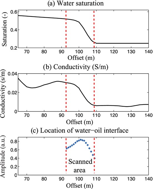
Determination of the position of the oil–water interface using a set of beamforming points at the same depth and crossing the position of the interface. (a) Spatial distribution of the water saturation (snapshot #3) showing the position of the saturation front. (b) Electrical conductivity distribution. (c) Source intensity as a function of offset. This shows that the strongest seismoelectric conversions are generated at the position of the saturation front.
6 CONCLUSIONS
We have developed a simple theory to compute seismoelectric effects in unsaturated conditions. This theory is based on the model of wave propagation in unsaturated media following a straightforward extension of Biot theory that is well accepted. We also developed an even simpler approach based a poroacoustic theory that is also used to compute P waves in partially saturated porous media. The electrokinetic part of the model is also consistent with available experimental observations in the laboratory.
The poroacoustic approach is implemented in a finite-element solver with triangular meshing. The capabilities of the forward modelling solver are shown in two cases. The first case is to perform seismic beamforming to localize the presence of heterogeneities in the saturation for a piecewise constant distribution of saturation. The second case corresponds to an enhanced oil-recovery problem. Water is injected in one well and oil is produced in the second well. We show that the seismoelectric method can be used to localize the saturation front using the beamforming approach proposed recently by Sava & Revil (2012). By focusing seismic energy at a given point, we sharply increase the amplitude of the seismoelectric interface response (seismoelectric conversion) with respect to coseismic fields. This is extremely important because, most of the time, the coseismic signals are much stronger, in terms of amplitude, and the seismoelectric conversion barely detectable.
Funding was provided by the Petroleum Institute of Abu Dhabi. We thank Seth Haines for fruitful discussions and Junwei Zhang for the two-phase flow simulations. Dr. T.K. Young is also thanked for his support at Mines. We thank the Editor Jeannot Trampert, J. Germán Rubino and an anonymous referee for their constructive comments.
REFERENCES
APPENDIX: CONDUCTIVITY IN UNSATURATED CONDITIONS
Like in the case of permeability, the properties Λ(sw) and F(sw) are expected to be breakable into the product of a value at saturation and a function of the saturation itself.
