


Abstract
To better understand and interpret seismoelectric measurements acquired over vadose environments, both the existing theory and the wave propagation modelling programmes, available for saturated materials, should be extended to partial saturation conditions. We propose here an extension of Pride's equations aiming to take into account partially saturated materials, in the case of a water–air mixture. This new set of equations was incorporated into an existing seismoelectric wave propagation modelling code, originally designed for stratified saturated media. This extension concerns both the mechanical part, using a generalization of the Biot–Gassmann theory, and the electromagnetic part, for which dielectric permittivity and electrical conductivity were expressed against water saturation. The dynamic seismoelectric coupling was written as a function of the streaming potential coefficient, which depends on saturation, using four different relations derived from recent laboratory or theoretical studies. In a second part, this extended programme was used to synthesize the seismoelectric response for a layered medium consisting of a partially saturated sand overburden on top of a saturated sandstone half-space. Subsequent analysis of the modelled amplitudes suggests that the typically very weak interface response (IR) may be best recovered when the shallow layer exhibits low saturation. We also use our programme to compute the seismoelectric response of a capillary fringe between a vadose sand overburden and a saturated sand half-space. Our first modelling results suggest that the study of the seismoelectric IR may help to detect a sharp saturation contrast better than a smooth saturation transition. In our example, a saturation contrast of 50 per cent between a fully saturated sand half-space and a partially saturated shallow sand layer yields a stronger IR than a stepwise decrease in saturation.
1 INTRODUCTION
Over the past two decades, seismoelectric imaging has spawned new interest, due to theoretical advances (Pride & Morgan 1991; Pride 1994; Pride & Haarsten 1996; Haartsen & Pride 1997), modelling developments (Hu et al.2007; Zyserman et al.2010; Schakel et al.2011, 2012; Ren et al.2012; Yamazaki 2012) and a series of successful field experiments (Butler 1996; Garambois & Dietrich 2001; Thompson et al.2005, 2007; Dupuis et al.2007; Haines et al.2007; Dupuis et al.2009). In theory, the seismoelectric method could combine the sensitivity of electrical methods to hydrological properties of the subsurface, such as porosity, with a high spatial resolution comparable to that of seismic surveys (Dupuis & Butler 2006; Haines et al.2007). In addition, it may also be sensitive to hydraulic permeability (Garambois & Dietrich 2002; Singer et al.2005). Seismoelectric signals may have several origins, but in this work we will restrict ourselves to the study of electrokinetically induced seismoelectric conversions. When a seismic wave propagates in a fluid-containing porous medium, seismoelectric signals arise from electrokinetic conversions occurring at the microscale; these signals are measurable at the macroscale, using dipole receivers either laid at the ground surface (Garambois & Dietrich 2001; Haines et al.2007; Jouniaux & Ishido 2012) or deployed in boreholes (Zhu et al.1999; Toksöz & Zhu 2005; Dupuis & Butler 2006; Dupuis et al.2009). Several applications were foreseen for both seismoelectric and electroseismic imaging in the fields of hydrogeophysics (Dupuis et al.2007) and hydrocarbon exploration (Thompson & Gist 1993; Thompson et al.2007). Seismoelectric imaging may indeed be successful at characterizing high permeability fracture networks (Mikhailov et al.2000; Hunt & Worthington 2000; Zhu & Toksöz 2003) and at resolving thin geological layers (Haines & Pride 2006). The theory for the coupled propagation of seismic and electromagnetic (EM) waves was reformulated by Pride (1994) for saturated porous media after previous attempts made by Frenkel (1944) and Neev & Yeatts (1989) and has not yet been extended to partial saturation conditions. However, the full range of water saturation encountered in the near-surface should be accounted for to help interpret seismoelectric measurements acquired over partially saturated environments (Dupuis et al.2007; Haines et al.2007). Water content is indeed thought to influence seismoelectric waveforms via different mechanisms, the most extreme example being the absence of coseismic signals in totally dry environments (Bordes et al.2009). As water content affects seismic velocity, seismic attenuation, electrical conductivity, EM propagation and diffusion, as well as the coupling coefficient, both the coseismic field and interface response (IR) properties are expected to vary with water saturation. Furthermore, saturation is also thought to control the amplitudes of seismoelectric signals generated at depth: for example, while conducting a seismoelectric survey over an unconfined aquifer, Dupuis et al. (2007) reported that the most prominent signal was generated at the water table, that is, at an interface displaying a large saturation contrast.
The main purpose of this work is to extend Pride's theory (Pride 1994) to unsaturated porous media. We consider here a pore space filled with a two-phase water/air mixture to investigate the seismoelectric response in vadose environments, but we hope this work will pave the way for studies in which other multiphasic pore fluids will be addressed (oil/water mixture, for example). In this paper, the parameters entering Pride's equations are explicitly described as functions of the water phase saturation Sw and the electrical formation factor F. We resort to the effective medium theory to express mechanical properties, such as the bulk and shear moduli; we also use it to derive fluid properties, such as the dynamic viscosity (Table 2). The medium's permittivity is derived using the complex refractive index method (CRIM; all acronyms used in this paper are summarized in Table 1 ) (Birchak et al.1974), while its conductivity is obtained by extending the conductivity derived by Pride (1994, eq. 242) to partial saturation conditions; this expression takes the surface conductivities into account. We combine this approach with the strategy introduced by Strahser et al. (2011), thus writing the dynamic seismoelectric coupling under partial saturation conditions as a function of the saturation-dependent streaming potential coefficient (SPC). The results obtained with four different laws describing the SPC (Perrier & Morat 2000; Guichet et al.2003; Revil et al.2007; Allègre et al.2010) are discussed.
Acronyms used throughout this paper.
| EDL | Electrical double layer |
| EM | Electromagnetic |
| IR | Interface response |
| ERT | Electrical resistivity tomography |
| ERV | Elementary representative volume |
| SPC | Streaming potential coefficient |
| CRIM | Complex refractive index method |
| GPR | Ground penetrating radar |
| EDL | Electrical double layer |
| EM | Electromagnetic |
| IR | Interface response |
| ERT | Electrical resistivity tomography |
| ERV | Elementary representative volume |
| SPC | Streaming potential coefficient |
| CRIM | Complex refractive index method |
| GPR | Ground penetrating radar |
Effective properties for a water–air mixture.
| Parameter | Sw dependence | Expression |
|---|---|---|
| Kf (Pa) | YES | Brie et al. (1995): |
| Kf(Sw) = |$(K_{{\rm w}}-K_{{\rm g}})S_{{\rm w}}^{5}+K_{{\rm g}}$| | ||
| ρf (kg m−3) | YES | Arithmetic average: |
| ρf(Sw) = (1 − Sw)ρg + Swρw | ||
| η (Pa s) | YES | Teja & Rice (1981): |
| |$\eta (S_{{\rm w}}) = \eta _{{\rm g}}(\eta _{{\rm w}}/\eta _{{\rm g}})^{S_{{\rm w}}}$| | ||
| b1 (Ns m−1) | NO | Computed for water only with Einstein–Stokes’ law. |
| ϵ (F m−1) | YES | CRIM: |
| |$\epsilon = \epsilon _{0}[(1-\phi )\sqrt{\kappa _{{\rm s}}}+\phi S_{{\rm w}} \sqrt{\kappa _{{\rm w}}}+\phi (1-S_{{\rm w}})\sqrt{\kappa _{{\rm g}}}]^{2}$| | ||
| α∞ | NO | Hydraulic (geometric) tortuosity. |
| Λ (m) | NO | Characteristic length of the microstructure. |
| ωt (rad s−1) | YES | |$\omega _{{\rm t}} = \frac{\eta (S_{{\rm w}})}{Fk_{0}\rho _{f}(S_{{\rm w}})}$| |
| Cem and Cos (S) | NO | Computed for water only using Pride's expressions. |
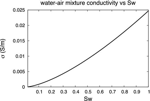
| σ (S m−1) | YES | σ(Sw, ω) = |$\frac{S_{{\rm w}}^{n}}{F}\sigma _{{\rm w}} + \frac{2}{F} \frac{C_{{\rm em}}+C_{{\rm os}}(\omega )}{\Lambda }$| |
| Parameter | Sw dependence | Expression |
|---|---|---|
| Kf (Pa) | YES | Brie et al. (1995): |
| Kf(Sw) = |$(K_{{\rm w}}-K_{{\rm g}})S_{{\rm w}}^{5}+K_{{\rm g}}$| | ||
| ρf (kg m−3) | YES | Arithmetic average: |
| ρf(Sw) = (1 − Sw)ρg + Swρw | ||
| η (Pa s) | YES | Teja & Rice (1981): |
| |$\eta (S_{{\rm w}}) = \eta _{{\rm g}}(\eta _{{\rm w}}/\eta _{{\rm g}})^{S_{{\rm w}}}$| | ||
| b1 (Ns m−1) | NO | Computed for water only with Einstein–Stokes’ law. |
| ϵ (F m−1) | YES | CRIM: |
| |$\epsilon = \epsilon _{0}[(1-\phi )\sqrt{\kappa _{{\rm s}}}+\phi S_{{\rm w}} \sqrt{\kappa _{{\rm w}}}+\phi (1-S_{{\rm w}})\sqrt{\kappa _{{\rm g}}}]^{2}$| | ||
| α∞ | NO | Hydraulic (geometric) tortuosity. |
| Λ (m) | NO | Characteristic length of the microstructure. |
| ωt (rad s−1) | YES | |$\omega _{{\rm t}} = \frac{\eta (S_{{\rm w}})}{Fk_{0}\rho _{f}(S_{{\rm w}})}$| |
| Cem and Cos (S) | NO | Computed for water only using Pride's expressions. |
| σ (S m−1) | YES | σ(Sw, ω) = |$\frac{S_{{\rm w}}^{n}}{F}\sigma _{{\rm w}} + \frac{2}{F} \frac{C_{{\rm em}}+C_{{\rm os}}(\omega )}{\Lambda }$| |
Effective properties for a water–air mixture.
| Parameter | Sw dependence | Expression |
|---|---|---|
| Kf (Pa) | YES | Brie et al. (1995): |
| Kf(Sw) = |$(K_{{\rm w}}-K_{{\rm g}})S_{{\rm w}}^{5}+K_{{\rm g}}$| | ||
| ρf (kg m−3) | YES | Arithmetic average: |
| ρf(Sw) = (1 − Sw)ρg + Swρw | ||
| η (Pa s) | YES | Teja & Rice (1981): |
| |$\eta (S_{{\rm w}}) = \eta _{{\rm g}}(\eta _{{\rm w}}/\eta _{{\rm g}})^{S_{{\rm w}}}$| | ||
| b1 (Ns m−1) | NO | Computed for water only with Einstein–Stokes’ law. |
| ϵ (F m−1) | YES | CRIM: |
| |$\epsilon = \epsilon _{0}[(1-\phi )\sqrt{\kappa _{{\rm s}}}+\phi S_{{\rm w}} \sqrt{\kappa _{{\rm w}}}+\phi (1-S_{{\rm w}})\sqrt{\kappa _{{\rm g}}}]^{2}$| | ||
| α∞ | NO | Hydraulic (geometric) tortuosity. |
| Λ (m) | NO | Characteristic length of the microstructure. |
| ωt (rad s−1) | YES | |$\omega _{{\rm t}} = \frac{\eta (S_{{\rm w}})}{Fk_{0}\rho _{f}(S_{{\rm w}})}$| |
| Cem and Cos (S) | NO | Computed for water only using Pride's expressions. |
| σ (S m−1) | YES | σ(Sw, ω) = |$\frac{S_{{\rm w}}^{n}}{F}\sigma _{{\rm w}} + \frac{2}{F} \frac{C_{{\rm em}}+C_{{\rm os}}(\omega )}{\Lambda }$| |
We also aim to provide the geophysical community with a comprehensive seismoelectric modelling programme enabling to simulate partial saturation conditions. Seismoelectric modelling programmes developed up to this day fall under one of two categories: they are either based on the general reflectivity method (Haartsen & Pride 1997; Garambois & Dietrich 2002) or they rely on finite-differences approaches (Haines & Pride 2006; Singarimbun et al.2008) or finite-elements approaches (Jardani et al.2010; Zyserman et al.2010; Kröger & Kemna 2012). Numerical codes based on finite differences enable to model seismoelectric signals acquired over 2-D media exhibiting lateral heterogeneities, but are limited to quasi-static approximations. On the other hand, the general reflectivity method enables to model the frequency-dependent seismoelectric response but is restricted to 1-D tabular media. All these codes are dealing only with full saturation conditions. A first attempt to model electroseismic waves in sandstones saturated with two-phase oil/water or gas/water mixtures was done by Zyserman et al. (2010). The authors resorted to an effective medium approach to compute the mixture's mechanical properties, that is, the mechanical properties of the effective fluid were established by performing a weighted average of those of the individual fluid phases. For the electrokinetic coupling, the electrical conductivity and the dielectric permittivity, the authors retained the values taken by these parameters in the wetting phase, that is, water. Jardani et al. (2010) were also able to model the forward seismoelectric response over a stratified medium including a reservoir partially saturated with oil. Following the approach introduced by Revil & Linde (2006), the authors modelled the problem by solving a system of quasi-static Poisson-type equations. For a partially water-saturated reservoir, the authors replaced the excess of charges by the excess of charges divided by water saturation. Within the frame of our study, we modify the semi-analytical programme of Garambois & Dietrich (2002) to account for partial saturation conditions. We study the modelled seismic and EM velocities and quality factors and the way they vary with water saturation. Three examples are presented here to illustrate seismoelectric signals variations with water saturation: the first model consists of a simple sand layer, whose saturation is allowed to vary, located on top of a saturated sandstone half-space. The second model consists of a sand layer of fixed saturation, but of varying thickness, on top of a sandstone saturated half-space. Finally, we use our modelling programme to simulate the seismoelectric response of a tabular model including a capillary fringe between an unsaturated sand overburden and a saturated half-space. This response is compared to the results obtained for a sharp saturation contrast between both units.
2 ELECTROKINETICALLY INDUCED SEISMOELECTRIC EFFECTS
The seismoelectric method relies on electrokinetically induced seismic-to-electric energy conversions occurring in fluid-containing porous media. These electrokinetic conversions are described at the microscale by the electrical double layer (EDL) theory (Gouy 1910; Chapman 1913; Stern 1924; Overbeek 1952; Dukhin & Derjaguin 1974; Davis et al.1978), which subdivides the pore fluid near the fluid/solid interface in a ‘bound’ layer where the charges in the electrolyte are adsorbed along the pore wall, and a diffuse layer, where these ions are free to move. A compressional wave travelling through such a medium creates a fluid-pressure gradient and an acceleration of the solid matrix, both of which induce a relative motion between the counter-ions in the diffuse layer and the immobile ions adsorbed at the grain surface. Counter-ions accumulate in compressional zones while bound layers are associated with zones of dilation. This charge separation at the scale of the seismic wavelet creates an electrical potential difference known as the streaming potential. The electric field arising from this potential is known as the ‘coseismic’ wave, as it travels within the passing compressional seismic waves. This electric field drives a conduction current that exactly balances the streaming current (through electron migration), which means there is no electric current within a compressional seismic wave travelling within a homogeneous medium. Therefore, as coseismic waves do not exist outside the seismic waves creating them, these waves may only help to characterize the medium near the receivers at the surface (Garambois & Dietrich 2001; Haines et al.2007; Bordes et al.2008), whereas for borehole seismoelectric measurements, they give information about the medium in the vicinity of the well (Mikhailov et al.2000).
Seismoelectric conversions are given birth when a seismic wave crosses a contrast between mechanical or electrical properties (Haartsen & Pride 1997; Chen & Mu 2005; Block & Harris 2006). This creates a transient localized charge separation across the interface, which acts as a secondary source that can be approximated as an electrical dipole oscillating at the first Fresnel zone (Thompson & Gist 1993, Fig. 1). The resulting EM wave, also known as the IR, diffuses independently from the seismic wavefield: the velocity at which it travels is several orders of magnitude greater than seismic velocities. This IR may provide information about the contrasts in the medium's properties at depth. However, IRs have typically very weak amplitudes and are often concealed by the stronger coseismic signals, as well as by ambient EM noise. This is indeed one of the key limitations of the seismoelectric method, which several authors tried to handle by extracting the IR from seismoelectric recordings through the use of various filtering techniques. Power-line noise is generally dealt with through block subtraction or sinusoidal subtraction (Butler 1993; Butler & Russell 2003). Coseismic waves are removed using dip-based techniques taking advantage of their relatively low velocity: these techniques include filtering in the frequency–wavenumber domain, Radon domain (Haines et al.2007; Strahser 2007) or curvelet domain (Warden et al.2012). Innovative acquisition layouts were also devised (Dupuis & Butler 2006; Haines et al.2007; Dupuis et al.2009), such as vertical seismoelectric profiling (VSEP): with these transmission geometries, source and receivers are placed on either side of the interface, which ensures separation between the coseismic waves and the IR.
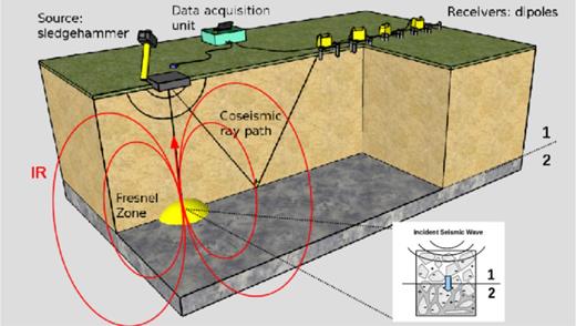
Typical seismoelectric survey acquisition geometry. When the incident seismic wave reaches an interface between two units of different mechanical, hydrological or electrical properties (denoted 1 and 2 in this figure), an Interface Response (IR) may arise from it. This signal originates below the shotpoint. Its radiation pattern is that of a dipole oscillating at the first Fresnel zone.
3 SEISMOELECTRIC DEPENDENCE ON WATER SATURATION
4 EXTENDING PRIDE's THEORY TO UNSATURATED CONDITIONS
4.1 A strategy combining an effective medium approach with SPC laws
In eq. (6), Λ (m) is a geometrical parameter of the pores, defined in Johnson et al. (1987), whereas p is a dimensionless parameter defined as p = |$\frac{\phi }{\alpha _{\infty } k_{0}} \Lambda ^{2}$| and consisting only of the pore-space geometry terms. This parameter p was originally denoted m in Pride (1994). When k0, ϕ, α∞ and Λ are independently measured, m is comprised between 4 and 8 for a variety of porous media ranging for grain packing to capillary networks consisting of tubes of variable radii (Johnson et al.1987). The parameter d (m) denotes the Debye length, while ωt (rad s−1) is the permeability-dependent transition angular frequency between the low-frequency viscous flow and high-frequency inertial flow. Finally, L0 denotes the electrokinetic coupling, whose expression will be discussed further. This coupling L(ω) was studied by Reppert et al. (2001), Schoemaker et al. (2007), Jouniaux & Bordes (2012) and Glover et al. (2012). When this coefficient is set to zero, the two subsets of equations describing the behaviour of EM and seismic waves are decoupled.
As previously pinpointed, Pride's equations have not yet been extended to partial saturation conditions. However, the behaviour of seismic waves in partially saturated porous media has been thoroughly studied, notably to explain seismic attenuation and waveform (Müller et al.2010). Laboratory experiments on sandstone (Knight & Dvorkin 1992) and limestone (Cadoret et al.1995) have shown that seismic attributes indeed depend on water saturation. Not only the water content, but also the way water fills the pore space influences seismic velocities, attenuation and dispersion (Knight & Nolen-Hoeksema 1990; Dvorkin & Nur 1998; Barrière et al.2012). The ‘patchy saturation’ model accounts for the heterogeneous mesoscale fluid distribution in the pore space: according to this model, under partial saturation conditions, patches of the porous medium are filled with gas, while other patches are filled with liquid. The distribution of the patches controls to which extent the mechanical properties of the medium deviate from those predicted by the Biot–Gassman theory. A simpler approach is offered by the effective medium theory, which states that the multiphasic fluid occupying the pore space can be replaced by a homogeneous fluid of equivalent effective properties (Gueguen & Palciauskas 1994). This approach allows to apply Biot's equations as if dealing with a biphasic solid/fluid medium. We will further discuss the mixing laws used to compute the medium's effective mechanical properties as a function of water saturation in Section 4.2. The effective medium approach, however, may not be blindly applied to determine all of the medium's properties. For instance, the electrical conductivity of a water/air mixture may not be computed as the weighted average of the conductivities of each individual phase, as under partial saturation conditions, the electrical current preferentially flows in the water phase: this calls for expressions of the saturation-dependent conductivity taking the formation factor into account. We will detail the laws used to compute the medium's electrical properties in unsaturated conditions in Section 4.3, bringing special attention to their frequency validity and to the rock types to which they apply. Other parameters, such as the ionic mobilities or the Debye length are intrinsically fluid-related and lose their meaning inside the air phase. For such parameters, we have chosen to use their values at full saturation.
4.2 Mechanical and fluid properties
4.2.1 Bulk modulus
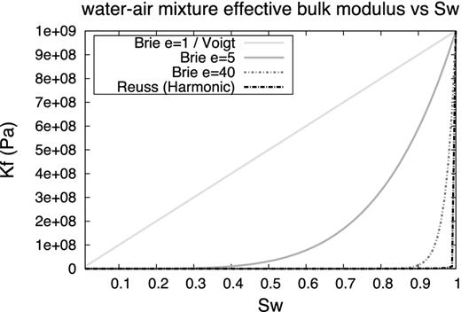
Effective bulk modulus Kf for a water–air mixture as a function of water saturation Sw. A water bulk modulus of Kw = 109 Pa was chosen, while a modulus of Kg = 105 Pa was taken for the gaseous phase.
4.2.2 Viscosity
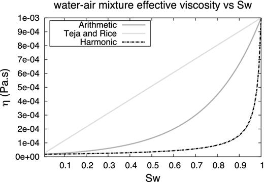
Effective viscosity η for a water–air mixture as a function of water saturation Sw. The air and water viscosity proposed by Ritchey & Rumbaugh (1996) are used here: ηg = 1.8 × 10⁻⁵ Pa s and ηw = 10−3 Pa s, respectively.
4.2.3 Mass density
4.3 EM properties
4.3.1 Dielectric constant
One may argue that the CRIM formula is valid when displacement currents dominate over conduction currents, but that this may no longer be the case at seismic or seismoelectric frequencies, that is, from tens of Hertz to hundreds of Hertz. The behaviour of the dielectric constant of sandstones versus water saturation at lower frequencies was investigated by several authors, between 5 Hz and 13 MHz (Knight 1984), 60 kHz and 4 MHz (Knight & Nur 1987) and between 0.1 Hz and 100 kHz (Gomaa 2008). Several authors have also studied the behaviour of the dielectric constant in sands and sandstones depending on whether the samples are submitted to imbibition or drainage: for instance, Plug et al. (2007) have measured the electric permittivity for sand–water–gas systems at 100 kHz and have found that the permittivity data show hysteresis between imbibition and drainage. While the dielectric constant values measured at several water saturation levels by Knight (1984) for a Berea sandstone at 13 MHz are of the same order of magnitude as those predicted with the CRIM formula, they are much higher at lower frequencies: for example, at 57 kHz for Sw = 0.9, the dielectric constant is about twice the one predicted using the CRIM formula (Knight 1984). At a frequency of 100 Hz, for a saturated clay-free haematitic sandstone, Gomaa (2008) measures a relative permittivity of about 2.4 × 10⁴, that is, more than 2000 times greater than the dielectric constant predicted by the CRIM formula on a similar sandstone. This increase of the dielectric constant with decreasing frequency could be explained by the Maxwell–Wagner relaxation model (Gueguen & Palciauskas 1994), for which the accumulation of electrical charges in the pore space is responsible for the dielectric dispersion observed at audiofrequencies. We conducted a sensitivity study for a simple half-space consisting of sands and found that increasing the dielectric constant by three orders of magnitude increased the EM wave velocity by 4 per cent, while increasing the maximum coseismic amplitude by less than 1 per cent. Following Zyserman et al. (2010), we chose to use the permittivity of the wetting phase, that is, water, in the expression of the seismoelectric coupling L0: this choice considerably reduces the impact of a change in permittivity on the seismoelectric amplitudes, which was confirmed by our sensitivity study. In the following, we will work under the assumption that these Maxwell–Wagner effects do not impact seismoelectromagnetic waveforms and we will compute the medium's relative permittivity using the CRIM formula.
4.3.2 Electrical conductivity
This approach combines Pride's frequency-dependent formula with Archie's law, developed under static conditions, to return conductivity as a function of both water saturation and frequency (Fig. 4). We assume here that the term 2/F × (Cem + Cos(ω))/Λ does not vary with water saturation Sw. According to Brovelli et al. (2005), the surface conductance Σs(S) should indeed be independent of the water saturation level. The authors explain that for Sw ≥ 0.15, the thickness of the wetting phase at the surface of the rock matrix is greater than the Debye length, that is, greater than the EDL thickness: therefore a saturation increase does not modify the properties of the EDL. It seems reasonable to make the same hypothesis here, because this work only aims to investigate a realistic range of saturation and assumes a non-negligible residual saturation Swr. To check that this residual saturation ensures the existence of the EDL, we modelled increasing saturation levels inside capillary pores which radii were comprised between 1 and 100 μm, assuming the wetting phase to grow from the pore walls towards the centre of the pore space (Allen 1996). We computed the thickness of the wetting phase (Fig. 5), which we compared to an analytical expression of the Debye length given by Pride (1994). It appears that for this simple pore geometry, for a salinity higher than 10−4 mol L−1 and saturation greater than 10 per cent, the thickness of the wetting phase is always greater than the Debye length, thus allowing us to assume the surface conductivity independent from Sw.
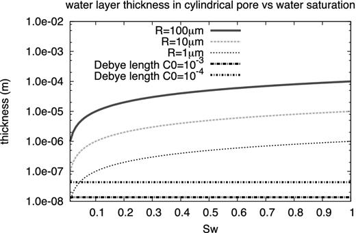
Comparison between the thickness of the wetting phase for cylindrical pores for various pore radii and the Debye length (m) computed for a salinity of C0 = 10−3 and C0 = 10−4 mol L−1, over the entire saturation range.
4.4 Expressing the electrokinetic coupling as a function of the SPC
Streaming potential coefficient (SPC) laws analysed throughout this study. S(Sw): function of saturation appearing in eq. (17). Swr denotes the residual saturation. n is Archie's saturation exponent.
| Reference | S(Sw) | Swr |
|---|---|---|
| Perrier & Morat (2000) | |$\frac{1}{S_{{\rm w}}^{n}}(\frac{S_{{\rm w}}-S_{{\rm wr}}}{1-S_{{\rm wr}}})^{2}$| | 0.10 |
| Guichet et al. (2003) | |$(\frac{S_{{\rm w}}-S_{{\rm wr}}}{1-S_{{\rm wr}}})$| | 0.10 |
| Revil et al. (2007) | |$\frac{1}{S_{{\rm w}}^{n+1}}(\frac{S_{{\rm w}}-S_{{\rm wr}}}{1-S_{{\rm wr}}})^{4}$| | 0.10 |
| Allègre et al. (2010) | |$(\frac{S_{{\rm w}}-S_{{\rm wr}}}{1-S_{{\rm wr}}})(1+32(1-(\frac{S_{{\rm w}}-S_{{\rm wr}}}{1-S_{{\rm wr}}}))^{0.4})$| | 0.305 |
4.5 Validation step
Parameters Kfr (Pa) and Ks (Pa) are the frame and solid bulk moduli, while Gfr (Pa) and Gs (Pa) denote the frame and solid shear moduli. For example, the solid shear modulus of quartz grains (Gs = 44 × 109 Pa), a porosity of 20 per cent and a consolidation of 20 yield a frame shear modulus Gfr of 5 × 10⁹ Pa.
We compared the results obtained using both the saturated version of our programme and the version developed for partially saturated conditions, for a simple tabular model consisting of a shallow sand layer over a sandstone half-space. We computed the velocities obtained using both programmes for the fast and slow P waves, S wave and EM wave travelling inside both layers. The seismic velocities computed with our code and those returned by the original programme were identical, while for the EM velocities, the deviation remained below 0.001 per cent. We also compared the maximum, minimum and mean amplitudes of the seismoelectric signals modelled using both our programme and its original version and found the same values using either tool. The electrograms modelled using both programmes appeared almost identical, with the residual between both recordings consisting only of non-coherent residual noise whose mean amplitude is less than 1 per cent the mean amplitude of the original recording. Finally, a full reciprocity test was successfully performed on the partially saturated programme.
5 PARTIALLY SATURATED SANDY OVERBURDEN ON TOP OF A FULLY SATURATED SANDSTONE HALF-SPACE
5.1 Model description
In the previous section, we verified that for a fully saturated porous medium, our modelling programme granted the same results than the original programme in terms of velocities, quality factors and amplitudes. We now investigate the seismoelectric response modelled with this programme over the entire ‘effective’ saturation Se range, that is, from the residual saturation Sw = Swr up to Sw = 1. We consider a tabular medium consisting of a 30-m thick sand layer on top of a sandstone half-space (Table 4). We allow the effective saturation in the sand overburden to vary from 0 to 1 with a 0.05 saturation increment. We model a vertical seismic source located near the surface, at a depth of 3 m, to simulate a downhole seismic gun shot. An array of 201 dipole receivers is modelled. Receivers are buried at a depth of 1 m between −50 and 50 m, with the origin set at the source location.
Properties of the model described in Section 5.
| Sand | Sandstone | |
|---|---|---|
| ϕ(%) | 35 | 20 |
| cs | 20 | 5 |
| m | 2.05 | 1.70 |
| k0 (m2) | 10−11 | 10−13 |
| ks (Pa) | 35 × 109 | 36 × 109 |
| Gs (Pa) | 44 × 109 | 44 × 109 |
| kf (Pa) | 2.27 × 10⁹ | 2.27 × 10⁹ |
| kfr (Pa) | 2.84 × 10⁹ | 14.40 × 10⁹ |
| Gfr (Pa) | 2.49 × 10⁹ | 14.08 × 10⁹ |
| ηw (Pa s) | 1 × 10⁻³ | 1 × 10⁻³ |
| ηg (Pa s) | 1.8 × 10⁻⁵ | 1.8 × 10⁻⁵ |
| ρs (kg m−3) | 2.6 × 10³ | 2.6 × 10³ |
| ρw (kg m−3) | 1 × 10³ | 1 × 10³ |
| ρg (kg m−3) | 1 | 1 |
| C0 (mol L−1) | 1 × 10⁻³ | 1 × 10⁻³ |
| σ (S m−1) | 1.32 × 10⁻³ | 7.54 × 10⁻⁴ |
| ζ (V) | −0.065 | −0.065 |
| κw | 80 | 80 |
| κs | 4 | 4 |
| κg | 1 | 1 |
| T (K) | 298 | 298 |
5.2 Velocity and attenuation analysis
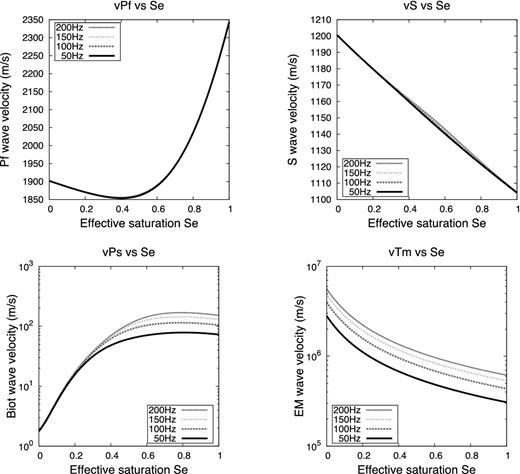
P wave, S wave, Biot slow wave and EM wave velocities as a function of effective saturation Se for the sand layer described in Table 4. These velocities were computed at 50, 100, 150 and 200 Hz. Note that the P-wave and S-wave velocities are plotted with a linear scale.
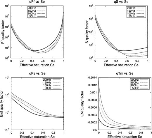
P wave, S wave, Biot slow wave and EM wave quality factors as a function of effective saturation Se for the sand layer described in Table 4. These quality factors were computed at 50, 100, 150 and 200 Hz. Note that the EM wave quality factor is plotted with a linear scale.
In eq. (22), s (S m−1) is the slowness of the considered wave. The quality factor Q quantifies the effect of anelastic attenuation on seismic or EM waves; the smaller the quality factor, the greater the absorption. Fast P-wave and S-wave quality factors vary dramatically with the effective saturation. For instance, QPf at 50 Hz decreases from 1.3 × 10⁵ to about 500 when Se increases from 0 to 0.45 before increasing again to 2.5 × 10⁶. On the other hand, for the frequency range investigated here, the EM quality factor variations are negligible: at 200 Hz, QEM only decreases between 0.5013 and 0.5 over the entire effective saturation range. This calls for a thorough investigation of the quality factor variations with frequency. For five saturation levels (20, 40, 60, 80 and 100 per cent), we plotted the quality factors against frequency f, with f ranging between 1 and 108 Hz (Fig. 8). The fast P waves and S waves display a similar behaviour, dictated by the fluid flow regime. For viscous fluid flow, that is, for f < 2πωt, their quality factor decreases as ωt/f: ωt denotes here the angular transition frequency, defined as |$(\eta S_{{\rm w}}^{m})/(Fk_{0}\rho _{f})$|. For inertial flows, that is, for f > 2πωt, QPf and QS increase as |$\sqrt{(f/\omega _{{\rm t}})}$|. Therefore, attenuation is greatest when f = 2πωt. It is interesting to note that the angular transition frequency ωt increases with saturation: for instance, ωt = 8.6 Hz for Sw = 20 per cent, whereas ωt = 11.6 kHz at full saturation. For Sw = 20 per cent, the curves for QPf and QS overlap, which means the attenuation is the same for both wave types. However, as saturation increases, the curve for QPf is shifted upwards, while the curve for QS remains unaffected by saturation changes. For the Biot slow P wave, the quality factor remains constant in the viscous regime. For f > 2πωt, QPs increases with the same slope as the other volume waves. On the other hand, the EM wave quality factor is not affected by the fluid flow type but instead depends on the regime type: it has a different behaviour whether or not diffusion dominates over propagation. QEM is weak (close to 0.5) and frequency- and saturation-independent in the conduction current dominant diffusive regime, that is, at low frequencies. It increases with frequency in the displacement current dominant propagative regime, that is, for high frequencies. For simple materials, the transition frequency between both regimes is given by f = σ(ω)/(2πϵ(ω)) (Rubin & Hubbard 2005) and is therefore saturation-dependent.
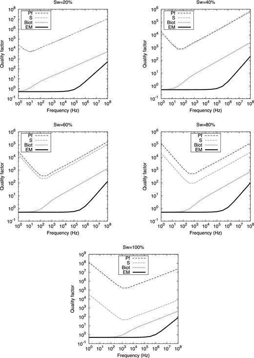
Seismic and electromagnetic quality factors versus frequency for 20, 40, 60, 80 and 100 per cent water saturation.
5.3 Amplitude analysis
We also studied the amplitudes of the seismoelectric signals modelled with our programme. While it had virtually no influence on velocities, the law chosen to compute the SPC directly influences the recovered amplitudes, which calls for a thorough comparison between the results granted by all four relations (Perrier & Morat 2000; Guichet et al.2003; Revil et al.2007; Allègre et al.2010). Like its previous version, our modelling programme is based on the equations of Kennett & Kerry (1979), enabling to simulate the seismic and EM response of a porous tabular medium. Among other advantages, this formalism allows to boost chosen conversions by multiplying specific coefficients in the reflectivity–transmissivity matrices by arbitrary pre-factors. Multiplying the Pf-EM, S-EM and Ps-EM coefficients by an arbitrary factor of 108 before normalizing the corresponding electrogram by the same value allows to model the IR without the pollution of the coseismic wavefield. Using this technique, we plotted the IR maximum amplitudes against saturation Sw, for all four SPC relations (left-hand side graph in Fig. 9). It appears that using the SPC laws of Perrier & Morat (2000), Guichet et al. (2003) and Revil et al. (2007), the maximum amplitude of the IR monotonically decreases with increasing saturation. The IRs modelled using these laws reach a maximum value of about 2.5 × 10⁻⁴ V at residual saturation Sw = 0.15 (Swr). They reach a minimum value of about 2.5 × 10⁻⁵ V at full saturation. As it could be expected, the IR follows a non-monotonic behaviour when using the relation introduced by Allègre et al. (2010). Its value increases from 8.8 × 10⁻⁵ V to a maximum value of 5.9 × 10⁻⁴ V when saturation increases from Sw = 0.35 up to a saturation close to 0.65, before decreasing with increasing saturation down to a value of 2.4 × 10⁻⁵ V at full saturation, about the same minimum value reached using the other laws. Therefore, the model of Allègre et al. (2010) returns the biggest IR amplitude of all four models (0.59 mV at Sw = 0.65).
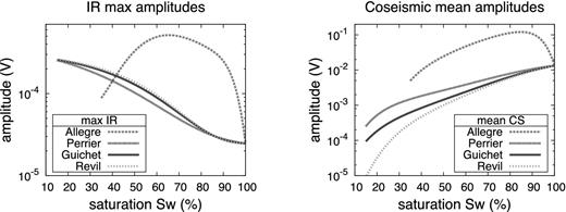
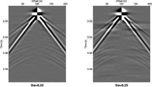
In our previous work, when using the original programme to create synthetic seismoelectric recordings for full saturation conditions (Warden et al.2012), we were never able to model an IR strong enough that it could be seen without subsequent filtering; we had to artificially amplify the IR with the technique mentioned above. This seemed problematic, as IRs, albeit very weak, have reportedly been measured in the field on several occasions (Haines et al.2007). We thought that maybe water saturation contrasts could be responsible for the difference between the IR amplitudes measured in the field and those modelled with our original programme. To verify this hypothesis, we also plotted the coseismic surface wave mean amplitudes against saturation along with the maximum IR amplitudes (right-hand side graph in Fig. 9). It turns out that, as saturation decreases, the coseismic surface wave mean amplitude decreases for the SPC laws of Perrier & Morat (2000), Guichet et al. (2003) and Revil et al. (2007) from 1.3 × 10⁻² V at full saturation, down to minimum values ranging from 8.7 × 10⁻⁶ V at Sw = 0.15 for the SPC derived from Revil et al. (2007) to 2.5 × 10⁻⁴ V for Perrier & Morat (2000). Therefore, as the water saturation falls down towards the residual saturation value Swr, both the decreasing coseismic amplitudes and the increasing IR amplitudes make it progressively easier to detect the IR. For instance, according to our amplitude analysis, using the SPC derived by Revil et al. (2007), one may only start distinguishing the IR below Sw = 0.35. Modelling the corresponding electrograms for Sw = 0.25 and Sw = 0.35 confirms this result (Fig. 10). On the other hand, the coseismic mean amplitude follows a ‘bell-shaped’ behaviour for the relation of Allègre et al. (2010): it increases from 1.3 × 10⁻² V at full saturation to nearly 1.5 × 10⁻¹ V at Sw = 0.90 before decreasing to 5.0 × 10⁻³ V at Sw = 0.35. In fact, for this set of parameters the IR maximum never exceeds the mean coseismic surface wave amplitude.
We also plotted the mean IR amplitude for a fixed saturation of a sand overburden (Sw = 0.4), whose thickness is allowed to increase from 5 to 50 m (Fig. 11). Quite unsurprisingly, the mean IR amplitude decreases with increasing thickness, mainly because the distance between the interface and the surface-located receivers increases. For instance, for the SPC law of Guichet et al. (2003) it decreases from 2.5 × 10⁻³ V at a depth of 5 m down to 9.3 × 10⁻⁶ V at a depth of 50 m. It turns out that, for shallow horizons, a change in the interface depth by only a few metres may modify the IR by an order of magnitude.
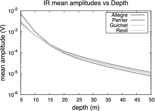
Interface response maximum amplitude values in the sand overburden as a function of the depth of the interface between the unsaturated sand layer (Sw = 40 per cent) and the fully saturated sandstone half-space. These results were modelled for the SPC laws of Perrier & Morat (2000), Guichet et al. (2003), Revil et al. (2007) and Allègre et al. (2010).
6 CAPILLARY FRINGE BETWEEN A SATURATED SAND HALF-SPACE AND A PARTIALLY SATURATED SAND OVERBURDEN
6.1 Model description
The simple subsurface layered models considered up to this point all simulate sharp saturation contrasts between consecutive units (Fig. 12a). In reality, instead of jumping from one value to the other, saturation may smoothly decrease with distance to the water table, due to capillary action. We use the partial saturation modelling programme to simulate such a capillary fringe between vadose and saturated sand layers (Table 5) by modelling a great number of very thin layers whose saturation increases by a small constant step from one layer to the other (Fig. 12b). In doing this, we adopt the definition according to which the unsaturated zone includes the capillary fringe: other authors may prefer to define the capillary fringe as being part of the saturated zone. We model here 100 layers, 0.5 cm thick, which saturation increases by Sw = 0.5 per cent from one layer to the next. The overburden has a water saturation of 50 per cent, while the fully saturated half-space simulates an aquifer (Sw = 1). The thickness of the capillary fringe is controlled by the pore sizes; it is generally less for coarse-grain materials than for fine-grain materials (Kaufman et al.2011). As it was reported to be less than 1 m thick in sands (Walker 2012), we chose to work with a capillary zone 0.5 m thick, embedded between 29.5 and 30 m. Seismic and seismoelectromagnetic waves are generated by a vertical source of peak frequency fpeak = 120 Hz, buried 3 m deep, and recorded by 201 receivers evenly spaced between x = −50 and 50 m.
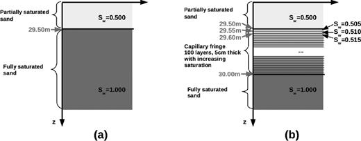
Tabular models used to simulate (a) a simple contact between a shallow unsaturated sand layer and a saturated sand half-space and (b) a capillary fringe between these two units. The capillary fringe is modelled by 100 thin unsaturated layers, 0.5 cm thick, which saturation increases with depth with a step of Sw = 0.5 per cent between two consecutive layers.
Properties of the model described in Section 6.
| Sand overburden | Sand half-space | |
|---|---|---|
| ϕ | 35 | 35 |
| cs | 20 | 20 |
| m | 2.05 | 2.05 |
| k0 (m2) | 10−11 | 10−11 |
| ks (Pa) | 35 × 109 | 35 × 109 |
| Gs (Pa) | 44 × 109 | 44 × 109 |
| kf (Pa) | 2.27 × 10⁹ | 2.27 × 10⁹ |
| kfr (Pa) | 2.84 × 10⁹ | 2.84 × 10⁹ |
| Gfr (Pa) | 2.49 × 10⁹ | 2.49 × 10⁹ |
| ηw (Pa s) | 1 × 10⁻³ | 1 × 10⁻³ |
| ηg (Pa s) | 1.8 × 10⁻⁵ | 1.8 × 10⁻⁵ |
| ρs (kg m−3) | 2.6 × 10³ | 2.6 × 10³ |
| ρw (kg m−3) | 1 × 10³ | 1 × 10³ |
| ρg (kg m−3) | 1 | 1 |
| C0 (mol L−1) | 1 × 10⁻³ | 1 × 10⁻³ |
| σ (S m−1) | 3.22 × 10⁻⁴ | 1.32 × 10⁻³ |
| ζ (V) | −0.065 | −0.065 |
| κw | 80 | 80 |
| κs | 4 | 4 |
| κg | 1 | 1 |
| T (K) | 298 | 298 |
| Sw | 0.5 | 1 |
6.2 Influence of the capillary fringe on the IR
We compared the horizontal electric field Ex generated both for a subsurface model exhibiting a sharp saturation contrast between the vadose and saturated sand layers (Fig. 12a) and a model including a capillary fringe (Fig. 12b). To recover the IR free from the coseismic waves, we proceeded as in Section 5.3, by multiplying the Pf-EM, S-EM and Ps-EM coefficients by an arbitrary factor before normalizing the resulting electrograms by the same value. Both seismoelectric recordings appear very similar (Fig. 13). They exhibit a first event of zero moveout around 45 ms, a time corresponding to the sum of the traveltime needed by the fast P wave to go from the source to the interface and for the converted EM wave to travel back to the receivers deployed at the ground surface. A second ‘flat’ event of lower magnitude appears around 68 ms: it corresponds to the converted S-EM wave.
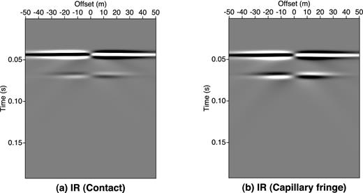
Although the IRs modelled with or without a capillary fringe closely resemble each other, their amplitudes are very different. We have computed the IR mean amplitude versus offset over a 25 samples window centred on the Pf-EM conversion (Fig. 13a) and the S-EM conversion (Fig. 13b). The Pf-EM IR obtained by modelling a capillary fringe consisting of 100 layers appears roughly 2.5 times weaker than the IR recovered by simulating a simple contact (Fig. 14): for a simple contact, the Pf-EM IR mean amplitude at offset x = 15 m is 3.4 × 10 −5 V, versus only 1.3 × 10⁻⁵ V for a 100 layers capillary fringe model. Modelling other capillary fringes using a smaller number of layers (e.g. 10 or 50 layers) yields the same result. On the other hand, the S-EM IR obtained for a tabular model including a capillary fringe is slightly stronger than the IR recovered for a simple contact between the vadose and saturated sand layers (4.5 × 10⁻⁶ V versus 4.0 × 10⁻⁶ V at offset x = 12 m). These results suggest that it would be harder to measure such an IR for a smooth saturation transition at the top of the water table than for a sharp saturation contrast between the vadose and saturated zones.
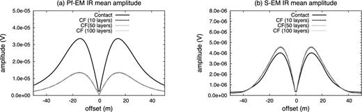
Interface Response mean amplitude distribution as a function of offset, for a simple contact (solid black line) and for several capillary models designed with a different numbers of layers (grey broken lines). (a) Pf-EM conversion. (b) S-EM conversion. The SPC law of Guichet et al. (2003) was used here. For the Pf-EM conversion, the models including a capillary fringe yield lower IR amplitudes than the model with a sharp saturation contrast.
7 CONCLUSION
In this paper, we extended Pride's theory originally developed to simulate seismoelectromagnetic wave conversions in fully saturated porous media to partial saturation conditions. To achieve this goal, mechanical, EM and coupling constitutive properties were computed for a water/air mixture. In particular, a generalization of Biot–Gassmann theory to the unsaturated case was performed through a simple homogenization technique. For the EM properties, we used the CRIM formula to determine the effective fluid permittivity and an extension of Pride's equation to compute the conductivity of the fluid in unsaturated rocks. The saturation-dependent electrokinetic coupling was tested using various laws experimentally derived to describe the behaviour of the SPC against water saturation. These changes have been incorporated into an existing seismoelectromagnetic wave propagation algorithm, originally developed to study seismoelectric properties in saturated stratified media. This new code is used to model the seismoelectric response of a simple tabular medium for which the saturation in the sand overburden is allowed to vary, while remaining constant in the underlying sandstone half-space. A thorough amplitude analysis reveals that, using the SPC laws of Perrier & Morat (2000), Guichet et al. (2003) and Revil et al. (2007), the amplitude ratio between the IR and the coseismic signal increases with decreasing water saturation of the shallow sandy layer. For instance, the IR maximum amplitude at full saturation is three orders of magnitude smaller than the coseismic mean amplitude, using the SPC law derived by Perrier & Morat (2000), which means that, for fully saturated media, the IR is very difficult to detect. On the other hand, using the same SPC law under residual saturation conditions, the IR maximum amplitude is five times greater than the coseismic mean amplitude. Therefore, an IR created by a saturation contrast may be easier to detect than a seismoelectric conversion occurring at the boundary between two fully saturated units. This result accounts for the amplitude contrasts between the IRs and the coseismic signals observed in the field over unsaturated environments, which could not be explained using the original version of the code, allowing to model only saturated conditions. On the other hand, the non-monotonic SPC law of Allègre et al. (2010) yields a greater maximum IR amplitude than the other three models: this maximum IR amplitude is reached at a saturation of Sw = 0.65. Furthermore, our extended programme is also used to model a capillary fringe at the top of a water table. This study suggests that such a smooth saturation transition may be harder to detect than a sharp saturation contrast between two consecutive layers, as Pf-EM IR amplitudes recovered for subsurface models including a capillary zone appear smaller than for models exhibiting a sharp contrast. On the other hand, S-EM IRs seem slightly stronger for capillary fringe models than for sharp saturation contrasts. This result suggests that seismoelectric imaging using S-wave sources may allow to detect smooth saturation transition zones.
Our developments open the possibility for further investigations beyond the scope of this paper. In future work, one should attempt to simulate seismoelectric wave propagation in complex multiphasic porous media with gas/brine or oil/brine mixtures filling the pore space. In this case, one would need to find another way to derive the saturation-dependent seismoelectric coupling L0(Sw) in the other mixtures, which may imply using other laws describing the SPC behaviour for complex multiphasic fluids (Moore et al.2004; Jackson 2010). Moreover, our programme will be able to model a wide variety of environments, such as temperate glaciers (Kulessa et al.2006). Finally, future studies about the transfer functions under unsaturated conditions are also needed and will be possible using our developments.
This work was supported by CNRS. As part of the TRANSient ElectroKinetics (TRANSEK) project, this work was supported by the French National Research Agency. The authors would like to thank Evert Slob and one anonymous reviewer for their comments. The authors would also like to thank Michel Dietrich for useful discussions. SW would like to thank Damien Jougnot and Philippe Leroy for their insightful tips.
REFERENCES
SUPPORTING INFORMATION
Additional Supporting Information may be found in the online version of this article:
Figure S1. Dielectric constant versus water saturation Sw as measured by Knight (1984) on Berea (ϕ = 19.7 per cent) sandstone samples and Gomaa (2008) for Aswan (ϕ = 23 per cent) sandstone. The dielectric constant computed with the CRIM formula for a sandstone (ϕ = 23 per cent) is also plotted for comparison.
Figure S2. Results of the reciprocity test described in subsection 1.2 (Supplementary Data).
Please note: Oxford University Press are not responsible for the content or functionality of any supporting materials supplied by the authors. Any queries (other than missing material) should be directed to the corresponding author for the article.
