Abstract

Inner core translation, with solidification on one hemisphere and melting on the other, provides a promising basis for understanding the hemispherical dichotomy of the inner core, as well as the anomalous stable layer observed at the base of the outer core—the so-called F-layer—which might be sustained by continuous melting of inner core material. In this paper, we study in details the dynamics of inner core thermal convection when dynamically induced melting and freezing of the inner core boundary (ICB) are taken into account.

If the inner core is unstably stratified, linear stability analysis and numerical simulations consistently show that the translation mode dominates only if the viscosity η is large enough, with a critical viscosity value, of order ∼3 × 1018 Pa s, depending on the ability of outer core convection to supply or remove the latent heat of melting or solidification. If η is smaller, the dynamic effect of melting and freezing is small. Convection takes a more classical form, with a one-cell axisymmetric mode at the onset and chaotic plume convection at large Rayleigh number. η being poorly known, either mode seems equally possible. We derive analytical expressions for the rates of translation and melting for the translation mode, and a scaling theory for high Rayleigh number plume convection. Coupling our dynamic models with a model of inner core thermal evolution, we predict the convection mode and melting rate as functions of inner core age, thermal conductivity, and viscosity. If the inner core is indeed in the translation regime, the predicted melting rate is high enough, according to Alboussière et al.'s experiments, to allow the formation of a stratified layer above the ICB. In the plume convection regime, the melting rate, although smaller than in the translation regime, can still be significant if η is not too small.

Thermal convection requires that a superadiabatic temperature profile is maintained in the inner core, which depends on a competition between extraction of the inner core internal heat by conduction and cooling at the ICB. Inner core thermal convection appears very likely with the low thermal conductivity value proposed by Stacey & Loper, but nearly impossible with the much higher thermal conductivity recently put forward by Sha & Cohen, de Koker et al. and Pozzo et al. We argue however that the formation of an iron-rich layer above the ICB may have a positive feedback on inner core convection: it implies that the inner core crystallized from an increasingly iron-rich liquid, resulting in an unstable compositional stratification which could drive inner core convection, perhaps even if the inner core is subadiabatic.

1 INTRODUCTION

In the classical model of convection and dynamo action in Earth's outer core, convection is thought to be driven by a combination of cooling from the core–mantle boundary (CMB) and light elements (O, Si, S, …) and latent heat release at the inner core boundary (ICB). Convection is expected to be vigorous, and the core must therefore be very close to adiabatic, with only minute lateral temperature variations (Stevenson 1987), except in very thin, unstable boundary layers at the ICB and CMB. To a large extent, seismological models are consistent with the bulk of the core being well-mixed and adiabatic, which supports the standard model of outer core convection. Yet seismological observations indicate the existence of significant deviations from adiabaticity in the lowermost ∼200 km of the outer core (Souriau & Poupinet 1991). This layer, sometimes called F-layer for historical reasons, exhibits an anomalously low VP gradient which is most probably indicative of stable compositional stratification (Gubbins et al.2008), implying that the lowermost 200 km of the outer core are depleted in light elements compared to the bulk of the core. This is in stark contrast with the classical model of outer core convection sketched above: in place of the expected thin unstable boundary layer, seismological models argues for a very thick and stable layer. Note also that the thickness of the layer, ∼200 km, is much larger than any diffusion length scales, even on a Gy timescale, which means that if real this layer must have been created, and be sustained, by a mechanism involving advective transport.

Because light elements are partitioned preferentially into the liquid during solidification, iron-rich melt can be produced through a two-stage purification process involving solidification followed by melting (Gubbins et al.2008). Based on this idea, Gubbins et al. (2008) have proposed a model for the formation of the F-layer in which iron-rich crystals nucleate at the top of the layer and melt back as they sink towards the ICB, thus implying a net inward transport of iron which results in a stable stratification. In contrast, Alboussière et al. (2010) proposed that melting occurs directly at the ICB in response to inner core internal dynamics, in spite of the fact that the inner core must be crystallizing on average. Assuming that the inner core is melting in some regions while it is crystallizing in others, the conceptual model proposed by Alboussière et al. (2010) works as follow: melting inner core material produces a dense iron-rich liquid which spreads at the surface of the inner core, while crystallization produces a buoyant liquid which mixes with and carries along part of the dense melt as it rises. The stratified layer results from a dynamic equilibrium between production of iron-rich melt and entrainment and mixing associated with the release of buoyant liquid. Analogue fluid dynamics experiments demonstrate the viability of the mechanism, and show that a stratified layer indeed develops if the buoyancy flux associated with the dense melt is larger (in magnitude) than a critical fraction (≃80 per cent) of the buoyancy flux associated with the light liquid. This number is not definitive because possibly important factors were absent in Alboussière et al. (2010)'s experiments (Coriolis and Lorentz force, entrainment by thermal convection from above, …) but it seems likely that a high rate of melt production will still be required.

A plausible way to melt the inner core is to sustain dynamically a topography that will bring locally the ICB at a potential temperature lower than that of the adjacent liquid core, which allows heat to flow from the outer core to the inner core. The melting rate is then limited by the ability of outer core convection to provide the latent heat absorbed by melting, and only a significant ICB topography can lead to a non-negligible melting rate. More recently, Gubbins et al. (2011) and Sreenivasan & Gubbins (2011) have proposed that localized melting of the inner core might be induced by outer core convection, but the predicted rate of melt production is too small to produce a stratified layer according to Alboussière et al. (2010)'s experiments. Furthermore, it is not clear that the behaviour observed in numerical simulations at slightly supercritical conditions would persist at Earth's core conditions.

Among the different models of inner core dynamics proposed so far (Jeanloz & Wenk 1988; Yoshida et al.1996; Karato 1999; Buffett & Wenk 2001; Deguen et al.2011), only thermal convection (Jeanloz & Wenk 1988; Weber & Machetel 1992; Buffett 2009; Deguen & Cardin 2011; Cottaar & Buffett 2012) is potentially able to produce a large dynamic topography and associated melting. Thermal convection in the inner core is possible if the growth rate of the inner core is large enough and its thermal conductivity low enough (Sumita et al.1995; Buffett 2009; Deguen & Cardin 2011). One possible mode of inner core thermal convection consists in a global translation with solidification on one hemisphere and melting on the other (Monnereau et al.2010; Alboussière et al.2010; Mizzon & Monnereau 2013). The translation rate can be such that the rate of melt production is high enough to explain the formation of the F-layer (Alboussière et al.2010). In addition, inner core translation provides a promising basis for understanding the hemispherical dichotomy of the inner core observed in its seismological properties (Tanaka & Hamaguchi 1997; Niu & Wen 2001; Irving et al.2009; Tanaka 2012). Textural change of the iron aggregate during the translation (Bergman et al.2010; Monnereau et al.2010; Geballe et al.2013) may explain the hemispherical structure of the inner core. Inner core translation, by imposing a highly asymmetric buoyancy flux at the base of the outer core, is also a promising candidate (Aubert 2013; Davies et al.2013) for explaining the existence of the planetary scale eccentric gyre which has been inferred from quasi-geostrophic core flow inversions (Pais et al.2008; Gillet et al.2009).

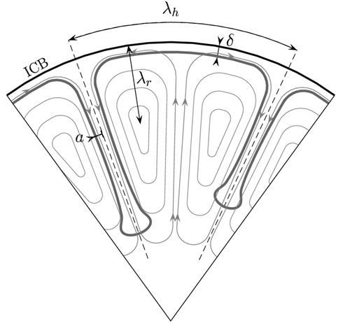
However, inner core translation induces horizontal temperature gradients (see Fig. 1), and Alboussière et al. (2010) noted that finite deformation associated with these density gradients is expected to weaken the translation mode if the inner core viscosity is too small. They estimated from an order of magnitude analysis that the threshold would be at η ∼ 1018 Pa s. Below this threshold, thermal convection is expected to take a more classical form, with cold plumes falling down from the ICB and warmer upwellings (Deguen & Cardin 2011). Published estimates of inner core viscosity range from ∼1011 to ∼1022 Pa s (Yoshida et al.1996; Buffett 1997; Van Orman 2004; Koot & Dumberry 2011; Reaman et al.2011, 2012) implying that both convection regime seem possible.

Figure 1.

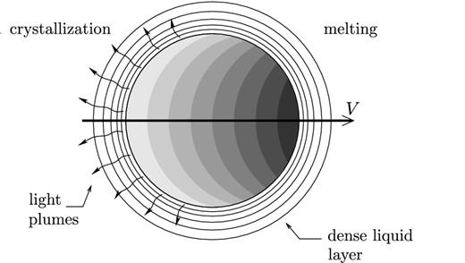
A schematic representation of the translation mode of the inner core, with the grey shading showing the potential temperature distribution (or equivalently the density perturbation) in a cross-section including the translation direction (adapted from Alboussière et al.2010).

The purpose of this paper is twofold: (i) to precise under what conditions the translation mode can be active, and (ii) to estimate the rate of melt production associated with convection, in particular when the effect of finite viscosity becomes important. To this aim, we develop a set of equations for thermal convection in the inner core with phase change associated with a dynamically sustained topography at the inner core boundary (Section 3). The kinetics of phase change is described by a non-dimensional number, noted |$\mathcal {P}$| for ‘phase change number’, which is the ratio of a phase change timescale (introduced in Section 2) to a viscous relaxation timescale. The linear stability analysis of the set of equations (Section 4) demonstrates that the first unstable mode of thermal convection consists in a global translation when |$\mathcal {P}$| is small. When |$\mathcal {P}$| is large, the first unstable mode is the classical one cell convective mode of thermal convection in a sphere with an impermeable boundary (Chandrasekhar 1961). An analytical expression for the rate of translation is derived in Section 5. We then describe numerical simulation of thermal convection, from which we derive scaling laws for the rate of melt production (Section 6). The results of the previous sections are then applied to the inner core, and used to predict the convection regime of the inner core and the rate of melt production as functions of the inner core growth rate and thermophysical parameters (Section 7).

2 PHASE CHANGE AT THE ICB

Any phase change at the ICB will release or absorb latent heat, with the rate of phase change v being determined by the Stefan condition,
\begin{equation} \rho _s L v = - [\![ q ]\!] _\mathrm{icb}, \end{equation}
(1)
which equates the rate of latent heat release or absorption associated with solidification or melting with the difference of heat flux [[q]]icb across the inner core boundary. Here ρs is the density of the solid inner core just below the ICB, and L is the latent heat of melting. The heat conducted along the adiabatic gradient on the outer core side is to a large extent balanced by the heat flow conducted on the inner core side, the difference between the two making a very small contribution to [[q]]icb. Convective heat transport in the inner core is small as well. Convection in the liquid outer core is a much more efficient way of providing or removing latent heat and − [[q]]icb is dominated by the contribution of the advective heat flux Φ(θ, ϕ) on the liquid side, which scales as
\begin{equation} \Phi \sim \rho _l c_{pl} u^{\prime } \delta \Theta , \end{equation}
(2)
where δΘ is the difference of potential temperature between the inner core boundary and the bulk of the core (Fig. 2), u is a typical velocity scale in the outer core, and ρl and cpl are the density and specific heat capacity of the liquid outer core in the vicinity of the inner core boundary (Alboussière et al.2010).
Figure 2.

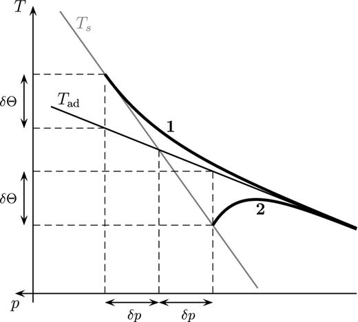
Temperature profiles (thick black lines) in the vicinity of the inner core boundary. Profile 1 corresponds to a crystallizing region, while profile 2 corresponds to a melting region. The thin black line is the outer core adiabat Tad and the thin grey line is the solidification temperature profile.

We choose as a reference radius the intersection of the mean outer core adiabat with the solidification temperature curve (Fig. 2), and note h(θ, ϕ) the distance from this reference to the inner core boundary. At a given location on the ICB, the difference of potential temperature between the ICB and the outer core is δΘ(θ, ϕ) = (mp − madp(θ, ϕ), where δp(θ, ϕ) is the pressure difference between the ICB and the reference surface (see Fig. 2), mp = dTs/dp is the Clapeyron slope, and mad = dTad/dp is the adiabatic gradient in the outer core. Taking into account the local anomaly Ψ of the gravitational potential (due to the ICB topography and internal density perturbations), we have from hydrostatic equilibrium δp = −ρl(gicbh + Ψ), which gives
\begin{equation} \delta \Theta = - (m_p - m_\mathrm{ad}) \rho _l g_\mathrm{icb} \left( h + \frac{\Psi ^{\prime } }{g_\mathrm{icb}} \right), \end{equation}
(3)
where gicb is the average gravity level on the surface of the inner core. The surface heq(θ, ϕ) = −Ψ/gicb is the equipotential surface which on average coincides with the ICB.
If the inner core is convecting, with a velocity field u(r, θ, ϕ, t) = (ur, uθ, uϕ), then the total rate of phase change is
\begin{equation} v = \dot{r}_\mathrm{ic} +\frac{ \partial h }{\partial t} - u_r , \end{equation}
(4)
where |$\dot{r}_\mathrm{ic}$| is the mean inner core growth rate, ric(t) being the inner core radius. Using eqs. (2)–(4), the heat balance (1) at the inner core boundary can be written as
\begin{equation} u_r - \dot{r}_\mathrm{ic} - \frac{\partial h }{\partial t} \sim \frac{ h + {\Psi ^{\prime } }/{g_\mathrm{icb}}}{\tau _\phi }, \end{equation}
(5)
where the timescale τϕ is
\begin{equation} \tau _\phi = \frac{\rho _s\, L}{\rho _l^2 c_{pl} \left( m_p - m_\mathrm{ad} \right) g_\mathrm{icb} u^{\prime } }. \end{equation}
(6)
With u ∼ 10−4 m s−1 and typical values for the other parameters (Table 1), the phase change timescale τϕ is found to be of the order of 103 years, which will turn out to be short compared to the dynamic timescale of thermal convection in the inner core (∼1 Myr or more). Noting Δρ = ρs − ρl, the viscous relaxation timescale τη = η/(Δρ gicbric) is at most ∼0.1 Myr (for η = 1022 Pa s), small as well compared to the inner core dynamic timescale. We therefore adopt the hypothesis of isostasy and neglect ∂h/∂t in (5), the heat transfer boundary condition finally adopted being written
\begin{equation} u_r - \dot{r}_\mathrm{ic} = \frac{ h + {\Psi ^{\prime } }/{g_\mathrm{icb}}}{\tau _\phi }, \end{equation}
(7)
where the unknown proportionality constant in eq. (2) has been absorbed in τϕ, and will be treated as an additional source of uncertainty.
Table 1.

Thermophysical parameters used in this study.

ParameterSymbolValue
Inner core radiusaricb1221 km
Solidification temperaturebTicb5600 ± 500 K
Gruneisen parametercγ1.4 ± 0.1
Thermal expansioncα(1.1 ± 0.1) × 10−5 K−1
Heat capacitydcp800 ± 80 J kg−1 K−1
Latent heat of meltingd, eL600–1200 kJ kg−1
Density jump at the ICBaΔρ600 kg m−3
Density in the inner coreaρs12 800 kg m−3
Density in the outer core at the ICBaρl12 200 kg m−3
Gravity at the ICBagicb4.4 m s−2
Radial gravity gradientag3.6 × 10−6 s−2
Thermal conductivityfk36–150 W m−1 K−1
Isentropic bulk modulusaKS1400 GPa
Clapeyron/adiabat slopes ratiogdTs/dTad1.65 ± 0.11

aFrom PREM (Dziewonski & Anderson 1981).

bAlfè et al. (2002).

cVočadlo (2007).

dPoirier (1994).

eAnderson & Duba (1997).

fStacey & Anderson (2001), Stacey & Davis (2008), Sha & Cohen (2011), de Koker et al. (2012) and Pozzo et al. (2012).

gDeguen & Cardin (2011).

3 GOVERNING EQUATIONS

3.1 Equations within the inner core

The starting point for the dynamics of thermal convection in the inner core is expressed as general entropy, momentum, continuity and gravitational equations:
\begin{eqnarray} \rho T \frac{\rm {}D s}{\rm {}D t} &= { {\nabla }} \cdot \left( k { {\nabla } } T \right) + \tau : \epsilon , \end{eqnarray}
(8)
\begin{eqnarray} {\bf 0} &= - { {\nabla } } p - \rho { {\nabla } } \Psi + { {\nabla } } \cdot \tau , \end{eqnarray}
(9)
\begin{eqnarray} 0 &= \displaystyle\frac{\partial \rho }{\partial t} + { {\nabla }} \cdot \left( \rho {\bf u} \right), \end{eqnarray}
(10)
\begin{eqnarray} {\nabla }^2 \Psi &= 4 \pi {\cal {G}} \rho , \end{eqnarray}
(11)
where ρ, T, s, k, τ, ϵ, p, Ψ and u denote density, temperature, specific entropy, thermal conductivity, shear-stress tensor, rate of deformation tensor, pressure, gravitational potential and velocity fields, respectively and where |${\cal {G}}$| is the universal gravitational constant. In eq. (9), inertia has been neglected and the gravity field g has been written using the gravitational potential |${\bf g} = - { {\nabla } } \Psi$|⁠.
These equations are then linearized around a state of well-mixed uniform but time dependent entropy, |$\overline{s}$|⁠, hydrostatic pressure |$\overline{p}$|⁠, density |$\overline{\rho }$|⁠, gravity |$\overline{\bf g}$| and gravitational potential |$\overline{\Psi }$| depending only on radius and time, such that |$\partial \overline{p}/ \partial r = -\overline{\rho }\, \overline{g}$|⁠, with |$\overline{\bf g}$| satisfying the gravitational equation |${\nabla }^2 \overline{\Psi } = 4 \pi {\cal {G}} \overline{\rho }$| and |$\overline{\bf g} = - { {\nabla } } \overline{\Psi }$|⁠. Linearized variables are introduced such that |$s=\overline{s}+s^{\prime }$|⁠, |$\rho = \overline{\rho } + \rho ^{\prime }$|⁠, |$T = \overline{T} + \Theta$|⁠, |$p = \overline{p} + p^{\prime }$|⁠, |$\Psi = \overline{\Psi } + \Psi ^{\prime }$| and |${\bf g} = \overline{{\bf g}} + {\bf g}^{\prime }$|⁠. |$\overline{T}(r)$| corresponds to an adiabatic profile, and |$\Theta =T-\overline{T}(r)$| is a potential temperature. The linearized governing equations take the form
\begin{eqnarray} \overline{\rho }\, \overline{T} \displaystyle\frac{D s^{\prime }}{D t} &= { {\nabla }} \cdot \left( k { {\nabla } } \Theta \right) + \tau : \epsilon - \overline{\rho }\, \overline{T} \displaystyle\frac{\partial \overline{s}}{\partial t} + { {\nabla }} \cdot \left( k { {\nabla } } \overline{T} \right), \end{eqnarray}
(12)
\begin{eqnarray} {\bf 0} &= - { {\nabla } } p^{\prime } - \overline{\rho} { {\nabla } } \Psi ^{\prime } - \rho ^{\prime } { {\nabla } } \overline{\Psi } + { {\nabla } } \cdot \tau , \end{eqnarray}
(13)
\begin{eqnarray} \nonumber\\\displaystyle\frac{\partial \rho ^{\prime }}{\partial t} &= -\displaystyle\frac{\partial \overline{\rho } }{\partial t}-{ {\nabla }} \cdot \left( \overline{\rho } {\bf u} \right), \end{eqnarray}
(14)
\begin{eqnarray} {\nabla }^2 \Psi ^{\prime } &= 4 \pi {\cal {G}} \rho ^{\prime }. \end{eqnarray}
(15)
Using Maxwell relations, we obtain a linearized expression of ρ in terms of s and p
\begin{equation} \rho ^{\prime } = \left( \frac{\partial \rho }{\partial s} \right)_{\!\!P} s^{\prime } + \left( \frac{\partial \rho }{\partial P} \right)_{\!\!s} p^{\prime } = - \frac{\overline{\alpha }\, \overline{\rho }\, \overline{T}}{\overline{c_p}} s^{\prime } - \frac{1}{\overline{\rho }\, \overline{\bf g}} \frac{\partial \overline{\rho }}{\partial r} p^{\prime }, \end{equation}
(16)
where |$\overline{\alpha }$| and |$\overline{c_p}$| are the volume expansion coefficient and specific heat capacity corresponding to the reference adiabatic state. With this expression for density fluctuations, eq. (13) can be written as
\begin{equation} {\bf 0} = - \overline{\rho } { {\nabla } } \left( \frac{p^{\prime }}{\overline{\rho }} + \Psi ^{\prime } \right) + \frac{\overline{\alpha }\, \overline{\rho }\, \overline{g} \, \overline{T}}{\overline{c_p}} s^{\prime } \, {\bf e_r} + { {\nabla } } \cdot \tau , \end{equation}
(17)
where er is the unit radial vector. The equation of entropy fluctuations (12) can be rewritten as
\begin{eqnarray} \overline{\rho }\, \frac{D\, \overline{T} s^{\prime }}{D t} &=& - \frac{\overline{\alpha } \overline{g} \overline{T} }{\overline{c_p}} s^{\prime } u_r + { {\nabla }} \cdot \left( k { {\nabla } } \Theta \right) + \tau : \epsilon - \overline{\rho }\, \overline{T} \frac{\partial \overline{s}}{\partial t}\nonumber \\ &&+\, { {\nabla }} \cdot \left( k { {\nabla } } \overline{T} \right). \end{eqnarray}
(18)
Then, the anelastic liquid approximation (Schubert et al.2001; Anufriev et al.2005) can be made, which consists in replacing the general linearized expression for entropy,
\begin{equation} s^{\prime }= \frac{\overline{c_p}}{\overline{T}} \Theta - \frac{\overline{\alpha }}{\overline{\rho }} p^{\prime }, \end{equation}
(19)
by its first term only,
\begin{equation} s^{\prime }\simeq \frac{\overline{c_p}}{\overline{T}} \Theta , \end{equation}
(20)
under the condition |$\overline{\alpha } \overline{T} Di \ll 1$| (Anufriev et al.2005), where |$Di = \overline{\alpha } \, g_\mathrm{icb} \, r_\mathrm{ic} / \overline{c_p}$| is the dimensionless dissipation number, which compares the inner core radius ric with the natural length scale for adiabatic temperature variations, |$\overline{c_p}/( \overline{\alpha } \, g_\mathrm{icb} )$|⁠. In the inner core, Di ≃ 0.07 × (ric/1221 km)2 and |$\overline{\alpha }\, \overline{T} \simeq 5\times 10^{-2}$|⁠, so that the anelastic liquid approximation can be made safely. An alternative analysis (Alboussière & Ricard 2013) indicates that cp/cv − 1 ≪ 1, where cv is the specific heat at constant volume, is the relevant criterion for the anelastic liquid approximation. Since cp/cv − 1 = γαT and the Gruneisen parameter γ is of order unity, this criterion is well satisfied. Under the liquid anelastic approximation, the momentum eq. (17) and entropy eq. (18) can then be written as
\begin{eqnarray} {\bf 0} &= - \overline{\rho }\, { {\nabla } } \left( \displaystyle\frac{p^{\prime }}{\overline{\rho }} + \Psi ^{\prime } \right) + \overline{\alpha }\, \overline{\rho }\, \overline{g}\, \Theta \, {\bf e_r} + { {\nabla } } \cdot \tau , \end{eqnarray}
(21)
\begin{eqnarray} \overline{\rho }\, \frac{{\rm {}D} \left( {\overline{c_p}} \Theta \right) }{{\rm {}D} t} &=& - \overline{\alpha } \overline{\rho } \overline{g} \Theta u_r + { {\nabla }} \cdot \left( k { {\nabla } } \Theta \right) + \tau : \epsilon \nonumber\\ && -\, \overline{\rho }\, \overline{c_p} \displaystyle\frac{\partial \overline{T}}{\partial t} + { {\nabla }} \cdot \left( k { {\nabla } } \overline{T} \right), \end{eqnarray}
(22)
where terms involving |$\partial \overline{c_p} / \partial t$| and |$\partial \overline{\rho } / \partial t$| have been neglected in (22).
The importance of self-gravitation is best estimated by analyzing its effect in terms of vorticity production. We form the vorticity equation by taking the curl of eq. (13), which gives
\begin{eqnarray} \mathbf {0} &= { {\nabla } }\bar{\rho }\times { {\nabla } } \Psi ^{\prime } + { {\nabla } } \rho ^{\prime } \times {\bar{\mathbf g}} + {\nabla } \times \left( { {\nabla } } \cdot \tau \right), \end{eqnarray}
(23)
\begin{eqnarray} = \displaystyle\frac{\rm {}d\bar{\rho }}{\rm {}d r} {\bf e_r} \times { {\nabla }_{\!h} } \Psi ^{\prime } - \bar{g}\, { {\nabla }_{\!h} } \rho ^{\prime } \times \mathbf {e_r} + {\nabla } \times \left( { {\nabla } } \cdot \tau \right), \end{eqnarray}
(24)
where |$ {\nabla }_{\!h}$| denotes the horizontal part of the gradient. The first term on the right-hand side originates from the interaction between the mean radial density gradient and the horizontal gradient in Ψ, and is to be compared with the second term, which results from the interaction between horizontal density gradients and the mean radial gravity field. From the gravitational equation, |${\nabla }^2 {\Psi ^{\prime }} = 4 \pi {\cal {G}} {\rho ^{\prime }}$|⁠, we find that |$\Psi ^{\prime } \sim 4\pi {\cal {G}} {\rho ^{\prime }} \lambda ^2$|⁠, where λ is the typical length scale of the temperature and gravitational potential perturbations. Using this estimate for Ψ the ratio of the first two terms in eq. (24) is
\begin{equation} \frac{\left| { {\nabla } }\bar{\rho }\times { {\nabla } } \Psi ^{\prime } \right|}{\left| { {\nabla } } \rho ^{\prime } \times \mathbf {\bar{g}} \right|} \sim \frac{\rm {}d \bar{\rho }}{{\rm {}d}{}r} \frac{\Psi ^{\prime }}{\bar{g} \rho ^{\prime }} \sim \frac{\rm {}d \bar{\rho }}{{\rm {}d}r}\frac{4\pi \mathcal {G} \lambda ^2}{\bar{g}}. \end{equation}
(25)
Noting that |${\rm d} \bar{\rho }/{\rm d}r = - ({\rm d} \bar{\rho }/{\rm d}p) \bar{\rho }\bar{g} = - \bar{\rho }^2 \bar{g}/K_S$| and that |$\bar{g}_\mathrm{icb}=(4\pi /3)\mathcal {G}\bar{\rho }\, r_\mathrm{ic}$|⁠, we obtain
\begin{equation} \frac{\left| { {\nabla } }\bar{\rho }\times { {\nabla } } \Psi ^{\prime } \right|}{\left| { {\nabla } } \rho ^{\prime } \times \mathbf {\bar{g}} \right|} \sim 3 \frac{\bar{\rho }\bar{g}_\mathrm{icb} r_\mathrm{ic}}{K_s} \frac{\lambda ^2}{r_\mathrm{ic}^2} \sim 3 \frac{Di}{\gamma } \frac{\lambda ^2}{r_\mathrm{ic}^2} , \end{equation}
(26)
where the Grüneisen parameter γ ≃ 1.4 is equal to |$\bar{\alpha }K_S/(\bar{c}_p \bar{\rho })$|⁠.

Since Di/γ ≃ 0.05, the vorticity source arising from self-gravitation effects might be up to ∼15 per cent of the total vorticity production if the length scale of convection is similar to the inner core radius, but has a much smaller contribution when λ/ric is small. Although the approximation might not be very good in cases where λ is comparable to ric, we will ignore here the radial variations of |$\bar{\rho }$|⁠, without which the force arising from self-gravitation is potential, and is therefore balanced by the pressure field. The density in the inner core is assumed to be uniform: |$\overline{\rho } = \rho _s$|⁠. To be consistent, |$\overline{g}$| is assumed to be a linear function of radius, |$\overline{g}=g_\mathrm{icb} r/r_\mathrm{ic}$|⁠. Density in the liquid outer core is assumed to be uniform as well: |$\overline{\rho _l} = \rho _l$|⁠. This is not correct for the outer core as a whole, but this is an excellent approximation within the depth range of the expected topography of the inner core boundary, so that ρl is the density of the outer core close to the inner core for our purpose.

The rheology is assumed to be Newtonian, with uniform effective viscosity η. Furthermore, viscous and adiabatic heating can be neglected since the dissipation number is small (Tritton 1988). We further assume that the thermal conductivity and thermal expansion are uniform. With |$\kappa = k/(\rho _s \, \overline{c_p})$| the thermal diffusivity, our final set of equation is
\begin{eqnarray} { {\nabla } } \cdot {\bf u} &= 0, \end{eqnarray}
(27)
\begin{eqnarray} {\bf 0} &= - { {\nabla } } \left( {p^{\prime }} + \rho _s \Psi ^{\prime } \right) + \displaystyle\frac{\overline{\alpha }\, \rho _s\,g_\mathrm{icb}}{r_\mathrm{ic}}\, \Theta \,r\, {\bf e_r} + {\eta } { {\nabla } }^2 {\bf u} , \end{eqnarray}
(28)
\begin{eqnarray} \frac{{\rm D} \Theta }{{\rm D} t} &= \kappa {\nabla }^2\ \Theta + S(t), \end{eqnarray}
(29)
where the effective heating rate S(t) is defined as the difference between secular cooling and heat conducted down the adiabat:
\begin{equation} S(t)= \kappa \nabla ^2 \overline{T} - \frac{\partial \overline{T}}{\partial t}. \end{equation}
(30)
S can be shown to depend mainly on time, not radius. When this term is positive (strong secular cooling and/or weak conduction), the inner core is superadiabatic and natural convection may develop.

3.2 Expression of boundary conditions

Despite the fact that we have stressed the necessity for a non uniform temperature on the inner core boundary when phase changes occur (in Section 2), we shall now argue that the boundary condition for thermal convection within the inner core is well approximated by Θ = 0 at r = ric. Indeed, the lateral variations of potential temperature associated with the ICB dynamic topography will be found to be of order 10−2 K or smaller (corresponding to a dynamic topography ≲100 m), while potential temperature variations within the inner core will be found to be of order 1 K or larger. We thus assume
\begin{equation} \Theta ( r=r_\mathrm{ic}) = 0. \end{equation}
(31)
The mechanical boundary conditions are tangential stress-free conditions (the fluid outer core cannot sustain tangential stress) and continuity of the normal stress at the inner core boundary. With the assumption of small topography, the normal vector is very close to the radial unit vector and the stress-free tangential conditions can be written as
\begin{eqnarray} \tau _{r \theta } = \eta \left[ r \frac{\partial }{\partial r} \left( \frac{u_\theta }{r} \right) + \frac{1}{r } \frac{\partial u_r}{\partial \theta } \right] &= 0 , \end{eqnarray}
(32)
\begin{eqnarray} \tau _{r \phi } = \eta \left[ r \frac{\partial }{\partial r} \left( \frac{u_\phi }{r} \right) + \frac{1}{r \sin \theta } \frac{\partial u_r}{\partial \phi } \right] &= 0 , \end{eqnarray}
(33)
where the spherical coordinates (r, θ, ϕ) are used, while the continuity of the normal stress gives
\begin{equation} \left[\!\left[ 2 \eta \frac{\partial u_r}{\partial r} - p \right]\!\right] _\mathrm{icb} = 0, \end{equation}
(34)
where [[…]]icb denotes the difference of a quantity across the ICB. Using again the decomposition |$p=\overline{p}+p^{\prime }$|⁠, this becomes
\begin{equation} \rho _l g_\mathrm{icb} h - p^{\prime +} - 2 \eta \frac{\partial u_r}{\partial r} - \rho _s g_\mathrm{icb} h + p^{\prime -} = 0, \end{equation}
(35)
where the subscripts + and − denote the liquid and solid sides respectively and where overlapping adiabatic hydrostatic states have been used for the liquid and solid regions. This condition can also be written as
\begin{equation} - \Delta \rho \, g_\mathrm{icb}\, h + \rho _l \Psi ^{\prime } - 2 \eta \frac{\partial u_r}{\partial r} + p^{\prime -} = 0, \end{equation}
(36)
because integrating the hydrostatic equation in the liquid outer core leads to p + ρlΨ constant, which applies also to perturbation quantities.

Finally, the radial velocity ur at the ICB is related to the topography h and gravitational potential perturbation Ψ through the heat balance at the ICB (eq. 7).

3.3 Set of equations

Introducing two new variables,
\begin{eqnarray} \hat{h} &= h + \displaystyle\frac{\Psi ^{\prime }}{g_\mathrm{icb}} , \end{eqnarray}
(37)
\begin{eqnarray} \hat{p} &= p^{\prime -} + \rho _s \Psi ^{\prime } , \end{eqnarray}
(38)
one can write the momentum and entropy equation, together with the boundary conditions relevant when phase change is allowed between solid inner core and liquid outer core:
\begin{eqnarray} { {\nabla } } \cdot {\bf u} &= 0, \end{eqnarray}
(39)
\begin{eqnarray} {\bf 0} &= - { {\nabla } } \hat{p} + \displaystyle\frac{\overline{\alpha }\, \rho _s\,g_\mathrm{icb}}{r_\mathrm{ic}}\, \Theta \, r\, {\bf e_r} + {\eta } { {\nabla } }^2 {\bf u} , \end{eqnarray}
(40)
\begin{eqnarray} \nonumber\\ \frac{{\rm D} \Theta }{{\rm D} t} &= \kappa {\nabla }^2 \Theta + S(t), \end{eqnarray}
(41)
with boundary conditions at r = ric from (31), (32), (33), (36) and (7):
\begin{eqnarray} \Theta &=0 , \end{eqnarray}
(42)
\begin{eqnarray} \tau _{r \theta } = \eta \left[ r \frac{\partial }{\partial r} \left( \frac{u_\theta }{r} \right) + \frac{1}{r } \frac{\partial u_r}{\partial \theta } \right] &= 0 , \end{eqnarray}
(43)
\begin{eqnarray} \tau _{r \phi } = \eta \left[ r \frac{\partial }{\partial r} \left( \frac{u_\phi }{r} \right) + \frac{1}{r \sin \theta } \frac{\partial u_r}{\partial \phi } \right] &= 0 , \end{eqnarray}
(44)
\begin{eqnarray} - \Delta \rho \, g_\mathrm{icb}\, \hat{h} - 2 \eta \frac{\partial u_r}{\partial r} + \hat{p} &= 0, \end{eqnarray}
(45)
\begin{eqnarray} u_r - \dot{r}_\mathrm{ic} &= \displaystyle\frac{ \hat{h} }{\tau _\phi }. \end{eqnarray}
(46)
It can be seen from (45) and (46), that |$\hat{h}$| is not necessary for the resolution of the equations, although it can be recovered once the problem is solved, and can be eliminated between these two equations, leaving only one boundary condition:
\begin{equation} - \Delta \rho g_\mathrm{icb} \tau _\phi ( u_r - \dot{r}_\mathrm{ic}) - 2 \eta \frac{\partial u_r}{\partial r} + \hat{p} = 0, \end{equation}
(47)
Incidently, it can also be seen that there is no need to explicitly solve the gravitational eq. (15), since Ψ has been absorbed in the modified pressure (38).
The governing equations and boundary conditions are now made dimensionless using the age of the inner core τic, its time dependent radius ric(t), κ/ric(t), |$\eta \kappa / r_\mathrm{ic}^2 (t)$| and |$S(t) r_\mathrm{ic}^2 (t) / (6 \kappa )$| as scales for time, length, velocity, pressure and potential temperature, respectively. Using the same symbols for dimensionless quantities, dimensionless equations can be written as
\begin{eqnarray} { {\nabla } } \cdot {\bf u} &= 0, \end{eqnarray}
(48)
\begin{eqnarray} {\bf 0} &= - { {\nabla } } \hat{p} + Ra(t)\, \Theta \, {\bf r} + { {\nabla } }^2 {\bf u} , \end{eqnarray}
(49)
\begin{eqnarray} \xi (t) \frac{\partial \Theta }{\partial t} &=& {\nabla }^2 \Theta - [{\bf u} -Pe (t) ] \cdot { {\nabla }} \Theta \nonumber\\ &&+\, 6 - \left[ \xi (t) \displaystyle\frac{{\skew4 \dot{S}} (t) \tau _{\mathrm {ic}}}{S (t) } + 2 \, Pe (t) \right] \Theta , \end{eqnarray}
(50)
where |${\bf r} = r\, \bf e_r$| and |${\skew4 \dot{S}} (t) = {\rm d} S(t) / {\rm d}t$|⁠. The last terms in (50) are due to dependency of the temperature scale on time, when used to make the equations dimensionless. Three dimensionless parameters are needed
\begin{eqnarray} \xi (t) &= \displaystyle\frac{r_\mathrm{ic}^2 (t)}{\kappa \tau _{\mathrm {ic}}}, \end{eqnarray}
(51)
\begin{eqnarray} Pe (t) &= \displaystyle\frac{r_\mathrm{ic} (t) \dot{r}_\mathrm{ic} (t) }{\kappa }, \end{eqnarray}
(52)
\begin{eqnarray} Ra (t) &= \displaystyle\frac{\alpha \rho _s g_\mathrm{icb}(t) S(t) r_\mathrm{ic}^5 (t) }{6 \kappa ^2 \eta }. \end{eqnarray}
(53)
The dimensionless boundary conditions, at r = 1, can be written
\begin{eqnarray} \Theta &=0 , \end{eqnarray}
(54)
\begin{eqnarray} \nonumber\\ \tau _{r \theta } = r \frac{\partial }{\partial r} \left( \frac{u_\theta }{r} \right) + \frac{1}{r } \frac{\partial u_r}{\partial \theta } &= 0 , \end{eqnarray}
(55)
\begin{eqnarray} \tau _{r \phi } = r \frac{\partial }{\partial r} \left( \frac{u_\phi }{r} \right) + \frac{1}{r \sin \theta } \frac{\partial u_r}{\partial \phi } &= 0 , \end{eqnarray}
(56)
\begin{eqnarray} - {\cal {P}} (t) ( u_r - \dot{r}_\mathrm{ic}) - 2 \frac{\partial u_r}{\partial r} + \hat{p} &= 0, \end{eqnarray}
(57)
where we have introduced the ‘phase change number’ |$\mathcal {P}$| characterizing the resistance to phase change:
\begin{equation} {\cal {P}} (t) = \frac{\Delta \rho \, g_\mathrm{icb} (t) \, r_\mathrm{ic} (t) \, \tau _\phi (t) }{\eta }. \end{equation}
(58)
|$\mathcal {P}$| is the ratio between the phase change timescale τϕ and the viscous relaxation timescale τη = η/(Δρ gicbric) (equivalent to postglacial rebound timescale). |$\mathcal {P}=0$| corresponds to instantaneous melting or freezing, while |$\mathcal {P}\rightarrow \infty$| corresponds to infinitely slow melting or freezing. In the limit of infinite |$\mathcal {P}$|⁠, the boundary condition (57) reduces to the condition ur = 0, which corresponds to impermeable conditions. In contrast, when |$\mathcal {P}\rightarrow 0$|⁠, eq. (57) implies that the normal stress tends towards 0 at the boundary, which corresponds to fully permeable boundary conditions. The general case of finite |$\mathcal {P}$| gives boundary conditions for which the rate of phase change at the boundary (equal to ur) is proportional to the normal stress induced by convection within the spherical shell.
A steady state version of the set of eqs (48)–(58) is found by using |$r_\mathrm{ic}^2/\kappa$| as a timescale instead of τic, and keeping ric and S constant. All the equation remain unchanged except the heat equation which now writes
\begin{equation} \frac{\partial \Theta }{\partial t} = {\nabla }^2 \Theta - {\bf u} \cdot { {\nabla }} \Theta + 6. \end{equation}
(59)
This will be used in Section 6 where numerical simulations with constant inner core radius and thermal forcing will be used to derive scaling laws.
With the assumptions made so far, the velocity field is known to be purely poloidal (Ribe 2007), and we introduce the poloidal scalar P defined such that
\begin{equation} {\bf u} = { {\nabla } } \times { {\nabla } } \times \left( P {\bf r} \right). \end{equation}
(60)
Taking the curl of the momentum eq. (49) gives
\begin{equation} Ra (t) L^2 \Theta = \left( {\nabla }^2 \right) ^2 L^2 P , \end{equation}
(61)
where the angular momentum operator L2 is
\begin{equation} L^2 = - \frac{1}{\sin \theta } \frac{\partial }{\partial \theta } \left( \sin \theta \frac{\partial }{\partial \theta } \right) - \frac{1}{\sin ^{2} \theta }\frac{ \partial ^2}{\partial \phi ^2}. \end{equation}
(62)
Horizontal integration of the momentum equation (see Forte & Peltier 1987; Ribe 2007, where this is done component-wise in spherical harmonics) shows that, on r = 1
\begin{equation} - \hat{p} + \frac{\partial }{\partial r } \left( r {\nabla }^2 P \right) = C^{{\rm st}}. \end{equation}
(63)
This expression can be used to eliminate |$\hat{p}$| in the boundary condition (57). Noting that
\begin{equation} u_r = \frac{1}{r} L^2 P, \end{equation}
(64)
continuity of the normal stress at the ICB (eq. 57) gives the following boundary condition at r = 1:
\begin{equation} \frac{\partial }{\partial r} \left( r {\nabla }^2 P - \frac{2}{r} L^2 P \right) - {\cal {P}} (t)\, \left( \frac{1}{r} L^2 P - \dot{r}_\mathrm{ic}\right) = C^{{\rm st}}, \end{equation}
(65)
while the stress-free conditions (55) and (56) take the form
\begin{equation} r \frac{\partial }{\partial r} \left[ \frac{1}{r^2} \frac{\partial }{\partial r} \left( r P \right) \right] + \frac{1}{r^2}L^2 P = C^{{\rm st}}, \end{equation}
(66)
which can be rewritten as
\begin{equation} \frac{\partial ^2 P}{\partial r^2} + \left( L^2 -{2} \right) \frac{P}{r^2} = C^{{\rm st}}. \end{equation}
(67)
At this stage, there are two unknown scalar field variables, Θ and P. They are expanded as
\begin{equation} \Theta = t_l^m (r,t)\, Y_l^m, \end{equation}
(68)
\begin{equation} P = p_l^m (r,t)\, Y_l^m, \ \ \ \ l \ge 1, \end{equation}
(69)
where |$Y_l^m (\theta , \phi )$|⁠, for l ≥ 0, m ∈ [−l; l] are surface spherical harmonics, which satisfy |$L^2 Y_l^m = l(l+1) Y_l^m$|⁠. The momentum eq. (61) takes the form
\begin{equation} Ra (t) t_l^m = \mathcal {D}_l^2 p_l^m , \end{equation}
(70)
where
\begin{equation} \mathcal {D}_l = \frac{{\rm d}^2 }{{\rm d} r^2} + \frac{2}{r} \frac{{\rm d}}{{\rm d} r} - \frac{l(l+1)}{r^2}. \end{equation}
(71)
The stress-free boundary condition (67) can be written as
\begin{equation} \frac{{\rm d}^2 p_l^m }{{\rm d} r^2} + \left[ l(l+1) -2 \right] \frac{p_l^m}{r^2} = 0, \ \ \ \ l \ge 1, \end{equation}
(72)
and the boundary condition (65), derived from normal stress balance, as
\begin{equation} \frac{{\rm d} }{{\rm d} r} \left[r \mathcal {D}_l p_l^m -2l(l+1) \frac{p_l^m}{r} \right] = l(l+1) {\cal {P}} (t) \frac{p_l^m}{r} , \ \ \ \ l \ge 1. \end{equation}
(73)
With (72), the equation above can also be written:
\begin{equation} r^2 \frac{{\rm d}^3 p_l^m }{{\rm d} r^3} -3 l (l+1) \frac{{\rm d} p_l^m }{{\rm d} r} = \left[ l(l+1) {\cal {P}} (t) -\frac{6}{r} \right]{p_l^m} , \ \ \ \ l \ge 1. \end{equation}
(74)
The thermal equation is also written in spherical harmonic expansion but cannot be solved independently for each degree and order due to the non-linearity of the advection term, which is evaluated in the physical space and expanded back in spherical harmonics.

4 LINEAR STABILITY ANALYSIS

We investigate here the linear stability of the system of equations describing thermal convection in the inner core with phase change at the ICB, as derived in Section 3. The calculation given here is a generalization of the linear stability analysis of thermal convection in an internally heated sphere given by Chandrasekhar (1961). The case considered by Chandrasekhar (1961), where a non-deformable, impermeable outer boundary is assumed, corresponds to the limit |$\mathcal {P}\rightarrow \infty$| of the problem considered here.

We assume constant Ra and |$\mathcal {P}$| (and ξ = 1, |$Pe={\skew4 \dot{S}} = 0$|⁠), thus ignoring that the base diffusive solution itself is time-dependent. This assumption is essentially correct when the growth rate of the fastest unstable disturbance is much larger than the growth rate of the radius of the inner core. The basic state of the problem is then given by
\begin{eqnarray} \bar{\Theta }&= 1 - r^2, \end{eqnarray}
(75)
\begin{eqnarray} \bar{ \mathbf {u}} &= \mathbf {0}, \end{eqnarray}
(76)
which is the steady conductive solution of the system of equation developed in Section 3. We investigate the stability of this conductive state against infinitesimal perturbations of the temperature and velocity fields. The temperature field is written as the sum of the conductive temperature profile given by eq. (75) and infinitesimal disturbances |$\tilde{\Theta }$|⁠, |$\Theta (r,\theta ,\phi ,t) = \bar{\Theta }(r) + \tilde{\Theta }(r,\theta ,\phi ,t)$|⁠. The velocity field perturbation is noted |$\tilde{\mathbf {u}}(r,\theta ,\phi ,t)$|⁠, and has an associated poloidal scalar |${\skew4 \tilde{P}}(r,\theta ,\phi ,t)$|⁠. We expand the temperature and poloidal disturbances in spherical harmonics,
\begin{eqnarray} \tilde{\Theta }= \sum _{l=0}^\infty \sum _{m=-l}^l \tilde{t}_l^m(r) Y_l^m(\theta ,\phi )\, \mathrm{e}^{\sigma _l t}, \end{eqnarray}
(77)
\begin{eqnarray} {\skew4 \tilde{P}} =\sum _{l=1}^\infty \sum _{m=-l}^l {\skew4 \tilde{p}}_l^m(r) Y_l^m(\theta ,\phi )\, \mathrm{e}^{\sigma _l t}, \end{eqnarray}
(78)
where σl is the growth rate of the degree l perturbations (note that since m does not appear in the system of equations, the growth rate is function of l only, not m).
The only non-linear term in the system of equations is the advection of heat u · ∇Θ in eq. (59), which is linearized as
\begin{equation} \tilde{u}_r \frac{\partial \bar{\Theta }}{\partial r} = -2 r \tilde{u}_r = - 2 L^2 {\skew4 \tilde{P}} . \end{equation}
(79)
The resulting linearized transport equation for the potential temperature disturbance is
\begin{equation} \left(\frac{\partial }{\partial t} - {\nabla }^2 \right)\tilde{\Theta }= 2 L^2{\skew4 \tilde{P}}. \end{equation}
(80)
Using the decompositions (77) and (78), the linearized system of equations is then, for l ≥ 1,
\begin{equation} Ra\, \tilde{t}_l^m = \mathcal {D}_l^2 {\skew4 \tilde{p}}_l^m, \end{equation}
(81)
\begin{equation} \left( \sigma _l - \mathcal {D}_l \right) \tilde{t}_l^m = 2 l (l+1) {\skew4 \tilde{p}}_l^m , \end{equation}
(82)
with the boundary conditions given by eqs (72) and (73), with |$\tilde{t}_l^m(r=1)=0$|⁠.
Developing the |$\tilde{t}_l^m$| in series of spherical Bessel functions and solving for |${\skew4 \tilde{p}}_l^m$|⁠, we obtain an infinite set of linear equations in perturbation quantities, which admits a non trivial solution only if its determinant is equal to zero (see Appendix A for the details of the calculation). This provides the following dispersion equation,
\begin{eqnarray} && \!\!\! \left|\left| \left[ q_3^l(\mathcal {P}) \alpha _{l,i}^2 + q_4^l(\mathcal {P}) \right] \left[1-\frac{4l+6}{\alpha _{l,j}^2} \right] -\left[ q_1^l(\mathcal {P}) \alpha _{l,i}^2 + q_2^l(\mathcal {P}) \right] \right.\right. \nonumber\\ &&+ \left.\left. \left( \frac{\sigma _l \alpha _{l,i}^4 + \alpha _{l,i}^6}{2l(l+1) Ra} - 1\right) \frac{1}{2} \delta _{ij} \right|\right| =0, \quad \text{with}\ \ i,j=1,2,\ldots\end{eqnarray}
(83)
where ||⋅⋅⋅|| denotes the determinant. Here αl, i denotes the ith zero of the spherical Bessel function of degree l. The functions |$q_1^l(\mathcal {P})$| to |$q_4^l(\mathcal {P})$| are given in Appendix A by eqs (A24), (A25), (A27) and (A28).
Solving eq. (83) for a given value of l and σl = 0 gives the critical value Rac of the Rayleigh number for instability of the degree l mode, as a function of |$\mathcal {P}$|⁠. The resulting marginal stability curves for l = 1–4 are shown in Fig. 3. The first unstable mode is always the l = 1 mode, for which eq. (83) reduces to
\begin{equation} \left|\left| \left(Ra - \frac{\alpha _{1,i}^6+\sigma _1 \alpha _{1,i}^4}{4 } \right) \delta _{ij} + {\alpha _{1,i}^2}\frac{Ra}{\mathcal {P} } +\frac{20}{3\, \alpha _{1,j}^2 }Ra \right|\right| = 0. \end{equation}
(84)
A useful first approximation is obtained by keeping only the i = j = 1 terms, thus setting the (1, 1) component of the matrix to zero. This gives a simple analytical form for the growth rate,
\begin{equation} \sigma _1 = \left( \frac{4}{\alpha _{1,1}^4} + \frac{80}{3\, \alpha _{1,1}^6} \right) Ra + \frac{4}{\alpha _{1,1}^2} \frac{Ra}{\mathcal {P}} - \alpha _{1,1}^2 \end{equation}
(85)
and for the critical Rayleigh number,
\begin{equation} Ra_c = \frac{\alpha _{1,1}^6}{4 } \left[ 1 + \frac{\alpha _{1,1}^2}{\mathcal {P} } + \frac{20}{3} \frac{1}{\alpha _{1,1}^2} \right]^{-1}, \end{equation}
(86)
with α1, 1 ≃ 4.4934. When |$\mathcal {P}\ll 1$| or |$\mathcal {P}\gg 1$|⁠, Rac and σl have the following limits:
\begin{eqnarray} Ra_c & \longrightarrow \left\lbrace \begin{array}{@{}l@{\quad }l@{}}\displaystyle{\frac{\alpha _{1,1}^8}{4\alpha _{1,1}^2 + 80/3 }} \simeq 1547 &{\rm when}\ \mathcal {P}\rightarrow \infty , \\ \displaystyle{\frac{\alpha _{1,1}^4}{4 } \mathcal {P}} \simeq 101.9\, \mathcal {P} &{\rm when} \ \mathcal {P}\rightarrow 0, \end{array}\right. \end{eqnarray}
(87)
\begin{eqnarray} \nonumber\\ \sigma _1 & \longrightarrow \left\lbrace \begin{array}{@{}l@{\quad }l@{}}\left(\displaystyle{\frac{4}{\alpha _{1,1}^4} + \frac{80}{3\, \alpha _{1,1}^6}} \right) Ra - \alpha _{1,1}^2\ & \quad{\rm when}\ \mathcal {P}\rightarrow \infty , \\ \displaystyle{\frac{4}{\alpha _{1,1}^2} \frac{Ra}{\mathcal {P}} - \alpha _{1,1}^2}\ & \quad{\rm when} \ \mathcal {P}\rightarrow 0, \end{array}\right. \end{eqnarray}
(88)
Higher order approximations can be obtained by retaining more terms in the determinant. For |$\mathcal {P}\gg 1$|⁠, the critical value of Ra converges towards
\begin{equation} Ra_c=1545.6, \end{equation}
(89)
in agreement with Chandrasekhar (1961)'s result (the value given by Chandrasekhar (1961) is twice the value given here, because of different definitions of Ra). When |$\mathcal {P}\ll 1$|⁠, the relevant non-dimensional parameter is the ratio |$Ra/\mathcal {P}$|⁠, which is independent of the viscosity and of the thermal diffusivity. An exact value of the critical value of |$Ra/\mathcal {P}$| will be given below (eq. 94).
Figure 3.

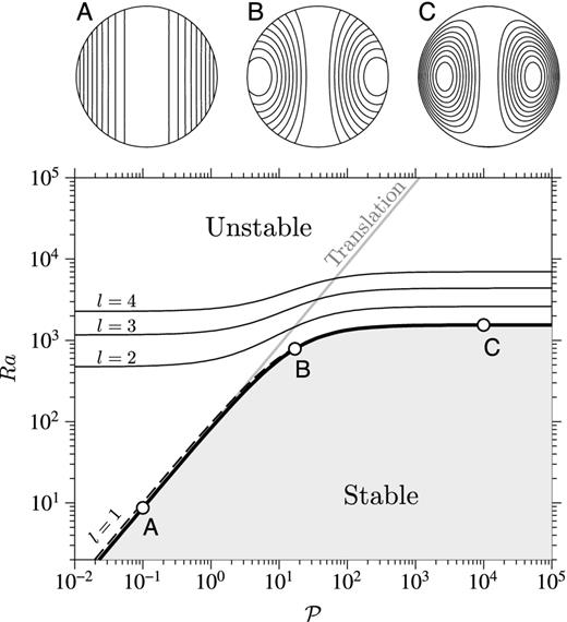
Stability diagram for convection in a sphere with phase change at its outer boundary. The neutral stability curve (l = 1) obtained by solving eq. (84) with σ1 = 0 is shown by the thick black line. The dashed line shows the approximate stability curve given by eq. (86). The neutral stability curves of higher modes (l = 2, 3, 4) obtained by solving eq. (83) with σl = 0 are shown by the annotated thin black lines. The neutral stability curves for l ≥ 5 are not shown to avoid overcrowding the figure. The thick grey curve annotated ‘Translation’ is the neutral stability curve of the translation mode, given by eq. (94). Streamlines of the first unstable mode at points A (⁠|$\mathcal {P} = 0.1$|⁠), B (⁠|$\mathcal {P} = 17$|⁠) and C (⁠|$\mathcal {P} = 10^4$|⁠) are shown in the upper figure.

The pattern of the first unstable mode can be calculated by solving the system (A39) given in Appendix A for given |$\mathcal {P}$| and Ra. The first unstable modes calculated in this way for points A, B and C (⁠|$\mathcal {P}=0.1$|⁠, 17 and 104) in the stability diagram are shown in Fig. 3. As shown in Appendix A, the l = 1, m ∈ [− 1, 0, 1] components of the poloidal scalar can be written as
\begin{eqnarray} {\skew4 \tilde{p}}_1^m = \sum _{i=1}^\infty A_{1,i} \left[ \frac{ j_1(\alpha _{1,i} r)}{\alpha _{1,i}} + \frac{j_2( \alpha _{1,i})}{3}( r - r^{3}) + \frac{ j_2( \alpha _{1,i})\alpha _{1,i}^2}{2\, \mathcal {P}} r \right], \nonumber \end{eqnarray}
(90)
where the coefficients A1, i are found by solving the system of eqs (A39). Here j1 and j2 denote the spherical Bessel functions of the first kind of order 1 and 2, respectively. From eq. (90), it can be seen that
\begin{equation} {\skew4 \tilde{p}}_1^m \rightarrow \left( \sum _{i=1}^{\infty } A_{1,i}\, j_2( \alpha _{1,i})\alpha _{1,i}^2 \right) \frac{2}{\mathcal {P}}r\quad {\rm when} \ \mathcal {P}\rightarrow 0, \end{equation}
(91)
which corresponds to a translation (it can be verified that a l = 1 flow with |$p_1^m \propto r$| corresponds to a flow with uniform velocity). This is the dominant mode when |$\mathcal {P}$| is small, as illustrated in Fig. 3 (point A, |$\mathcal {P}=0.1$|⁠). There is no deformation associated with this mode.

At high |$\mathcal {P}$|⁠, the term in |$1/\mathcal {P}$| in eq. (90) becomes negligible, and the first unstable mode is identical to the classical single cell degree one mode of thermal convection with shear-free boundary and no phase change (Chandrasekhar 1961), as illustrated in Fig. 3 (point C, |$\mathcal {P}=10^4$|⁠). There is no melting or solidification associated with this mode, which is apparent from the fact that the streamlines of the flow are closed. At intermediate values of |$\mathcal {P}$|⁠, the first unstable mode is a linear combination of the high-|$\mathcal {P}$| convection mode and of the small-|$\mathcal {P}$| translation mode.

Allowing only for the translation (i.e. keeping only the |$p_{1,i} \propto r/\mathcal {P}$| terms), the dispersion relation (84) reduces to
\begin{equation} \left|\left| \delta _{ij} - \frac{4}{\alpha _{1,i}^4} \frac{Ra}{\mathcal {P} } \right|\right| = 0. \end{equation}
(92)
Using Sylvester's determinant theorem, we find that
\begin{equation} \left|\left| \delta _{ij} - \frac{4}{\alpha _{1,i}^4} \frac{Ra}{\mathcal {P} } \right|\right| = 1 - 4 \frac{Ra}{\mathcal {P} } \sum _{i=1}^\infty \frac{1}{\alpha _{1,i}^{4}}, \end{equation}
(93)
which allows to write the critical value of |$Ra/\mathcal {P}$| as
\begin{equation} \left(\frac{Ra}{\mathcal {P}}\right)_{\!\!c} =\frac{1}{4} \left( \sum _{i=1}^\infty \frac{1}{\alpha _{1,i}^{4}} \right)^{-1} = \frac{175}{2}=87.5, \end{equation}
(94)
where we have used Sneddon (1960)'s result that |$\sum _{i=1}^\infty \alpha _{1,i}^{-4}=1/350$|⁠. The critical value 175/2 is exact, and is to be preferred to the approximate value (101.9) obtained in eq. (87). Eq. (94) gives the marginal stability curve shown in grey in Fig. 3. Although the translation mode can be unstable at all value of |$\mathcal {P}$| provided that Ra is large enough, it is apparent in Fig. 3 that the one cell convection mode is the first unstable mode whenever |$\mathcal {P}$| is larger than |$\simeq\!\! Ra_c/(Ra/\mathcal {P})_c \simeq 17$| (point B in Fig. 3).

Finally, it can be seen in Fig. 3 that the critical Rayleigh number |$Ra_c^l$| for higher order modes (l > 1) is also lowered when |$\mathcal {P}\lesssim 17$|⁠. However, the decrease in |$Ra_c^l$| is not as drastic as it is for the l = 1 mode because, whatever the value of |$\mathcal {P}$|⁠, viscous dissipation always limits the growth of these modes. The effect of |$\mathcal {P}$| on |$Ra_c^l$| becomes increasingly small as l increases. This suggests that allowing for phase change at the ICB would generally enhance large scale motions at the expense of smaller scale motions.

5 ANALYTICAL SOLUTIONS FOR SMALL |$\mathcal {P}$|

We now search for a finite amplitude solution of inner core convection at small |$\mathcal {P}$|⁠. In the limit of infinite viscosity (⁠|$\mathcal {P}\rightarrow 0$|⁠), the only possible motions of the inner core are rotation, which we do not consider here, and translation. Guided by the results of the linear stability analysis, we search for a solution in the form of a translation. Alboussière et al. (2010) found a solution for the velocity of inner core translation from a global force balance on the inner core, under the assumption that the inner core is rigid. One of the goal of this section is to verify that the system of equations developed in Section 3 indeed leads to the same solution when |$\mathcal {P}\rightarrow 0$|⁠.

If the viscosity is taken as infinite and |$\mathcal {P}$| is formally put to zero, searching for a pure translation solution and ignoring any deformation in the inner core leads to an undetermined system. Translation is an exact solution of the momentum equation, but the translation rate is left undetermined, because all the terms in the boundary conditions (55), (56) and (57) (zero tangential stress and continuity of the normal stress) vanish. This of course does not mean that the stress magnitude vanishes, but rather that the rheological relationship between stress and strain via the viscosity becomes meaningless if the viscosity is assumed to be infinite. The ICB topography associated with the translation is sustained by the non-hydrostatic stress field which, even if η → ∞, must remain finite. One way to calculate the stress field is to evaluate the flow induced by the lateral temperature variations associated with the translation, for small but non-zero |$\mathcal {P}$|⁠, and then take the limit |$\mathcal {P}\rightarrow 0$|⁠. If only the ‘rigid inner core’ limit is wanted, it suffices to calculate the flow at |$\mathcal {O}(\mathcal {P})$|⁠. The effect of finite viscosity on the translation mode can be estimated by calculating the velocity field at a higher order in |$\mathcal {P}$|⁠.

5.1 Translation velocity at zeroth order in |$\mathcal {P}$|

Noting V0 the translation velocity at zeroth order in |$\mathcal {P}$|⁠, the poloidal scalar takes the form
\begin{equation} p_1^0 = \frac{V_0}{2} \ r, \end{equation}
(95)
with |$Y_1^0 = \cos \theta$|⁠, in a cylindrical coordinate system of axis parallel to the velocity translation. If V0 is large enough, the temperature eq. (50) has a fast convective solution whereby |${\bf u} \cdot { {\nabla }} \Theta$| balances the constant 6. Imposing Θ = 0 at the ICB on the crystallizing hemisphere, and ignoring a thin boundary layer below the ICB on the melting hemisphere, the temperature field, shown in Fig. 4, is
\begin{equation} \Theta = \frac{6}{V_0} \left( r\, \cos \theta + \sqrt{1 - r^2 \sin ^2 \theta } \right) \end{equation}
(96)
(Alboussière et al.2010). This results in a uniform temperature gradient in the translation direction, with the l = 1, m = 0 component of the temperature field being
\begin{equation} t_1^0 = \frac{6}{V_0} \ r. \end{equation}
(97)
This temperature field induces a secondary l = 1, m = 0 flow which must vanish when |$\mathcal {P}\rightarrow 0$|⁠. We therefore write |$p_1^0$| as
\begin{equation} p_1^0 = \frac{V_0}{2}\left[ r + \hat{p}_{1,1}^0 \mathcal {P} + \mathcal {O}(\mathcal {P}^2) \right]. \end{equation}
(98)
Inserting this form for |$p_1^0$| and the temperature degree one component |$t_1^0$| into the momentum eq. (70) gives
\begin{equation} 12 \frac{Ra}{\mathcal {P}} \frac{1}{V_0^2} r = \mathcal {D}_1^2 \hat{p}_{1,1}^0, \end{equation}
(99)
from which we can already infer that
\begin{equation} V_0 \sim \sqrt{\frac{Ra}{\mathcal {P}}}. \end{equation}
(100)
Eq. (99) has a general solution of the form
\begin{equation} \hat{p}_{1,1}^0 = A r + B r^3 + C r^5, \end{equation}
(101)
where A, B and C are constants to be determined.
Figure 4.

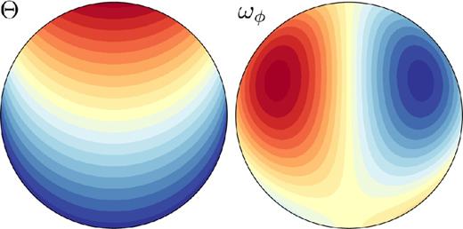
Temperature field (left, red = hot, blue = cold) and vorticity field at |$\mathcal {O}(\cal {P})$| (right, blue = negative, red = positive) in a meridional cross-section (the direction of translation is arbitrary).

From the momentum eq. (99), we obtain
\begin{equation} C = \frac{3}{70} \frac{Ra}{\mathcal {P}}\frac{1}{V_0^2} . \end{equation}
(102)
The stress-free boundary condition (72) for a degree one component,
\begin{equation} \left.\frac{d^2 p_1^0 }{d r^2}\right|_{r=1} = 0, \end{equation}
(103)
leads to
\begin{equation} B = - \frac{10}{3} C = - \frac{1}{7} \frac{Ra}{\mathcal {P}} \frac{1}{V_0^2} . \end{equation}
(104)
Finally, the condition of continuity of the normal stress (74) leads to
\begin{equation} \left( -3 B + 18 C - 1 \right) \mathcal {P} - 2 \mathcal {P}^2 (A+B+C) + \mathcal {O}(\mathcal {P}^2 ) = 0, \end{equation}
(105)
which implies that
\begin{equation} -3 B + 18 C - 1 = 0. \end{equation}
(106)
Note that the constant A is left undetermined: considerations of the velocity field at order |$\mathcal {P}^2$| and of the temperature field at order |$\mathcal {P}$| are required to determine it. With B and C given by eqs (104) and (102), eq. (106) gives the translation velocity V0 as
\begin{equation} V_0 = \sqrt{\frac{6}{5} \frac{Ra }{{\cal {P}}}}. \end{equation}
(107)
In dimensional unit, the translation rate is given by
\begin{equation} \frac{\kappa }{r_\mathrm{ic}}\sqrt{\frac{6}{5} \frac{Ra }{{\cal {P}}}} = \left( \frac{1}{5} \frac{\rho _s}{\Delta \rho } \frac{\alpha S }{ \tau _\phi } \right)^{1/2} r_\mathrm{ic} \end{equation}
(108)
which, with τϕ given by eq. (6), is exactly the same solution as that found in Alboussière et al. (2010) from an analysis of the global force balance on the inner core. As expected, the translation rate is independent of the inner core viscosity η and of the thermal diffusivity, and is an increasing function of the heating rate S and a decreasing function of the phase change timescale.
The potential temperature difference across the inner core is 12/V0 in non-dimensional units, and
\begin{equation} 12 \frac{S r_\mathrm{ic}^2}{6 \kappa } \left( \frac{5}{6} \frac{\mathcal {P}}{Ra} \right)^{1/2} = \left( 20 \frac{\Delta \rho \, \tau _\phi \, S}{\rho _s\, \alpha } \right)^{1/2} \end{equation}
(109)
in dimensional units.

5.2 Translation velocity at |$\mathcal {O}(\mathcal {P})$|

The translation velocity at |$\mathcal {O}(\mathcal {P})$| can be obtained by calculating the temperature field at |$\mathcal {O}(\mathcal {P})$| and the velocity field at |$\mathcal {O}(\mathcal {P}^2)$|⁠, which allows to determine the constant A in the expression of the poloidal scalar at |$\mathcal {O}(\mathcal {P})$| (eq. 101). The procedure, detailed in Appendix B, is complicated by the non-linearity of the heat equation: coupling of higher order harmonics component of the temperature and velocity fields contribute to the l = 1 component of the temperature field. Taking into account the effect of the non-linear coupling of the l = 2 components of the temperature and velocity fields, we obtain
\begin{equation} V = \sqrt{\frac{6}{5} \frac{Ra }{{\cal {P}}}} \left[ 1 - 0.0216\, \mathcal {P} + \mathcal {O}(\mathcal {P}^2) \right]. \end{equation}
(110)
which suggests that the effect of deformation becomes important when |$\mathcal {P}$| is a significant fraction of 1/0.0216 ≃ 46, in agreement with the prediction of the linear stability analysis.

The temperature field and the ϕ-component of the vorticity field at |$\mathcal {O}(\mathcal {P})$|⁠, as calculated in Appendix B, are shown in figure (4).

5.3 The effect of the boundary layer

Let us finally discuss the influence of the thermal boundary layer that must develop in the solid inner core near the melting side when a convective translation exists. From the thermal eq. (50), and with the boundary condition (54), a thermal boundary layer of thickness V −1 results from the balance between convective and diffusive terms, so that the degree one temperature component (97) may be approximated by
\begin{equation} t_1^0 \simeq \frac{6}{V} \left[ r - e^{ V (r-1) } \right] . \end{equation}
(111)
We now note that
\begin{equation} \mathcal {D}_1 \left[ \mathrm{e}^{V(r-1)} \right] = \left( 1 + \frac{2}{V r} - \frac{2}{V^2 r^2} \right) V^2 \mathrm{e}^{V(r-1)}, \end{equation}
(112)
so that to a good approximation,
\begin{equation} \mathcal {D}_1 \left[ \mathrm{e}^{V(r-1)} \right] \simeq V^2 \mathrm{e}^{V(r-1)}\quad {\rm and}\quad \mathcal {D}_1^2 \left( \mathrm{e}^{Vr} \right) \simeq V^4 \mathrm{e}^{V(r-1)} \end{equation}
(113)
when V ≫ 1. Under this assumption, the resulting general solution for the velocity poloidal component (101) becomes
\begin{eqnarray} p_1^0 \simeq \frac{V_0}{2}\left\lbrace r + \left[Ar + B r^3 + C r^5 - 10 \frac{V_0^2}{V^6} \mathrm{e}^{V (r-1)} \right] \mathcal {P}+ \mathcal {O}(\mathcal {P}^2) \right\rbrace .\nonumber\\ \end{eqnarray}
(114)
Following the same path as above, in the limit of infinite viscosity, the translation velocity V is found to be
\begin{equation} V \simeq V_0 \left( 1 - \frac{5}{V_0} - \frac{5}{V_0^2} + \frac{30}{V_0^3} - \frac{30}{V_0^4} \right) \end{equation}
(115)
when the effect of the boundary layer is taken into account.

5.4 Melt production

We define the rate of melt production |${\skew4 \dot{M}}$| as the volume of melt produced at the surface of the inner core by unit area and unit of time, averaged over the ICB. In the case of a pure translation, the volume of melt produced by unit of time is simply given by the translation velocity V multiplied by the cross-section |$\pi r_\mathrm{ic}^2$| of the inner core, so |${\skew4 \dot{M}}$| is given by
\begin{equation} {\skew4 \dot{M}} = \frac{V \times \pi r_\mathrm{ic}^2}{4 \pi r_\mathrm{ic}^2} = \frac{V}{4}. \end{equation}
(116)
For a more general inner core flow, |${\skew4 \dot{M}}$| can be calculated from the radial velocity at the ICB as
\begin{equation} {\skew4 \dot{M}} = \frac{1}{2} \overline{{|u_r(r_\mathrm{ic}) - \dot{r}_\mathrm{ic}|}} = \frac{1}{8 \pi } \int _{\theta ,\phi } |u_r(r_\mathrm{ic}) - \dot{r}_\mathrm{ic}| \sin \theta \, {\rm d}\theta {\rm d}\phi , \end{equation}
(117)
where the overbar |$\overline{\dots }$| denotes the average over a spherical surface. In the case of a l = 1, m = 0 flow, this reduces to
\begin{equation} {\skew4 \dot{M}} = \frac{1}{4 \pi } \int _{\theta ,\phi } |p_1^0 \cos \theta | \sin \theta \, {\rm d}\theta {\rm d}\phi = \frac{1}{2} |p_1^0| \end{equation}
(118)
and gives |${\skew4 \dot{M}}=V/4$| for a pure translation, which has |$p_1^0=V/2$|⁠.

6 NUMERICAL RESULTS AND SCALING LAWS

6.1 Method

The code is an extension of the one used in Deguen & Cardin (2011), with the boundary condition derived in Section 3 now implemented. The system of equations derived in Section 3 is solved in 3-D, using a spherical harmonic expansion for the horizontal dependence and a finite difference scheme in the radial direction. The radial grid can be refined below the ICB if needed. The non-linear part of the advection term in the temperature equation is evaluated in the physical space at each time step. A semi-implicit Crank- Nickolson scheme is implemented for the time evolution of the linear terms and an Adams–Bashforth procedure is used for the non-linear advection term in the heat equation. The temperature field is initialized with a random noise covering the full spectrum. We use up to 256 radial points and 128 spherical harmonics degree. Care has been taken that the ICB thermal boundary layer, which can be very thin in the translation mode, is always well resolved.

The code has the ability to take into account the growth of the inner core and the evolution of the internal heating rate S(t), which is calculated from the thermal evolution of the outer core (Deguen & Cardin 2011). In this section, we will first focus on simulations with a constant inner core radius and steady thermal forcing (internal heating rate S constant). Simulations with an evolving inner core will be presented in Section 7.

Each numerical simulation was run for at least 10 overturn times ric/Urms, where Urms is the rms velocity in the inner core.

6.2 Overview

As already suggested by the linear stability analysis (Section 4) and the small |$\mathcal {P}$| analytical model (Section 5), the translation mode is expected to be dominant when |$\mathcal {P}$| is small. This is confirmed by our numerical simulations. As an example, Fig. 5 shows outputs of simulations with the same Rayleigh number value of Ra = 107 and |$\mathcal {P}=1$|⁠, 30, 102 and 103. Snapshots of cross-sections of the potential temperature field and vorticity (its component perpendicular to the cross-section plane) are shown in the first and second columns, and maps of radial velocity ur(ric) at the ICB are shown in the third column. ur(ric) is equal to the local phase change rate, with positive values corresponding to melting and negative values corresponding to solidification.

Figure 5.

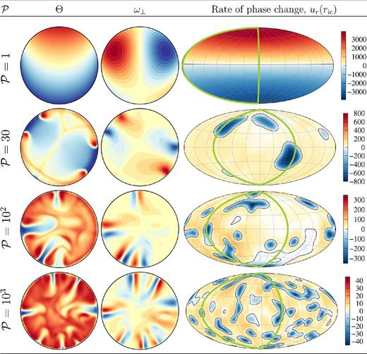
Snapshots from numerical simulations with Ra = 107 and |$\mathcal {P}=1$|⁠, 30, 100 and 103, showing potential temperature Θ (first column), azimuthal vorticity ω (second column) and radial velocity ur(ric) at the outer boundary (third column).

At the lowest |$\mathcal {P}$| (⁠|$\mathcal {P}=1$|⁠), the translation mode is clearly dominant, with the pattern of temperature and vorticity similar to the predictions of the analytical models of Section 5 shown in Fig. 4. In contrast, the convection regime at the largest |$\mathcal {P}$| (⁠|$\mathcal {P}=10^3$|⁠) appears to be qualitatively similar to the regime observed with impermeable boundary conditions (Weber & Machetel 1992; Deguen & Cardin 2011), which corresponds to the limit |$\mathcal {P}\rightarrow \infty$|⁠. At the Rayleigh number considered here, convection is chaotic and takes the form of cold plumes originating from a thin thermal boundary layer below the ICB, with a passive upward return flow. At intermediate values of |$\mathcal {P}$| (⁠|$\mathcal {P}=30$| and 102), phase change has still a significant effect on the pattern of the flow, with large scale components of the flow enhanced by phase change at the ICB, in qualitative agreement with the prediction of the linear stability analysis. Note that at |$\mathcal {P}=10^2$|⁠, there is still a clear hemispherical pattern, with plumes originating preferentially from one hemisphere.

More quantitative informations on the structure of convection can be found by estimating a characteristic length scale of the flow. We calculate here the mean degree |${\skew4 \bar{\ell }}_u$| of the flow from the time averaged kinetic energy spectrum, defined by Christensen & Aubert (2006) as
\begin{equation} {\skew4 \bar{\ell }}_u = \frac{\sum _\ell \ell E_k^\ell }{E_k}, \end{equation}
(119)
where
\begin{equation} E_k^\ell = \frac{1}{2} \sum _m (u_\ell ^m)^{2}\quad {\rm and}\quad E_k = \sum _\ell E_k^\ell . \end{equation}
(120)
With this definition, |${\skew4 \bar{\ell }}_u\rightarrow 1$| if the flow is dominated by degree 1 components, as in the translation mode, and increases as the characteristic length scale of the flow decreases.

Fig. 6 shows the calculated value of |${\skew4 \bar{\ell }}$| for Ra = 104, 105, 106 and 107 as a function of |$\mathcal {P}$|⁠. |${\skew4 \bar{\ell }}$| remains very close to 1 as long as |$\mathcal {P}$| is smaller than a transitional value |$\mathcal {P}_t\simeq 29$|⁠. There is a rapid increase of |${\skew4 \bar{\ell }}_u$| above |$\mathcal {P}_t$|⁠, showing the emergence of smaller scale convective modes at the transition between the translation mode and the high-|$\mathcal {P}$| regime. We interpret this sharp transition as being due to the negative feedback that the secondary flow and smaller scale convection have on the translation mode: advection of the potential temperature field by the secondary flow decreases the strength of its degree one component and therefore weakens the translation mode, which in turn give more time for smaller scale convection to develop, weakening further the degree one heterogeneity. The value of |$\mathcal {P}_t$| does not seem to depend on Ra in the range explored here. Fig. 6 further shows that ICB phase change has a strong influence on the flow up to |$\mathcal {P}\simeq 300$|⁠, which is confirmed by direct visualization of the flow structure.

Figure 6.

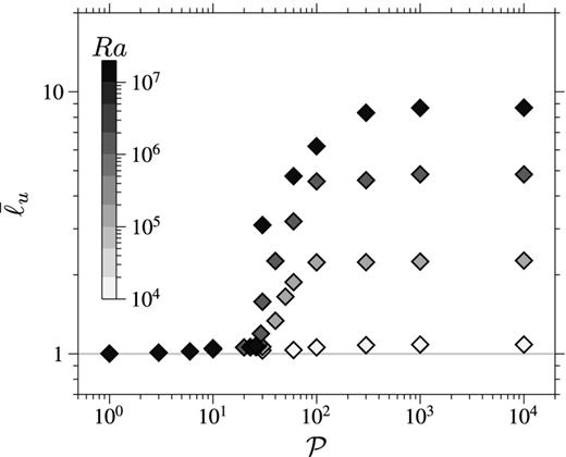
Mean degree |${\skew4 \bar{\ell }}_u$| of the kinetic energy (as defined in eq. 119), as a function of |$\mathcal {P}$|⁠, for simulations with Ra = 104, 105, 106 and 107. The grey scale of the markers give the Rayleigh number of the simulation. |${\skew4 \bar{\ell }}_u$| is close to 1 for |$\mathcal {P}\lesssim 29$| for all Ra, although the departure from 1 increases with Ra when |$\mathcal {P}$| approaches 29 from below.

Fig. 7a shows the translation rate V (circles) and time averaged rms velocity (triangles) as a function of |$\mathcal {P}$| for various values of Ra. Here both V and Urms are multiplied by Ra−1/2. The grey dashed line shows the analytical prediction for the translation rate in the rigid inner core limit. Below |$\mathcal {P}_t$|⁠, there is a good quantitative agreement between the numerical results and the analytical model. The fact that UrmsV for |$\mathcal {P}<\mathcal {P}_t$| indicates that there is, as expected, negligible deformation in this regime. V and Urms diverge for |$\mathcal {P}>\mathcal {P}_t$|⁠, the translation rate becoming rapidly much smaller than the rms velocity. As already suggested by the evolution of |${\skew4 \bar{\ell }}$|⁠, phase change at the ICB has still an effect on the convection for |$\mathcal {P}$| up to ∼300. Phase change at the ICB has a positive feedback on the vigor of the convection: melting occurs preferentially above upwelling, where the dynamic topography is positive, which enhances upward motion. Conversely, solidification occurs preferentially above downwellings, thus enhancing downward motions. This effect becomes increasingly small as |$\mathcal {P}$| is increased, and the rms velocity reaches a plateau when |$\mathcal {P}\gtrsim 10^3$|⁠, at which the effect of phase change at the ICB on the internal dynamics becomes negligible.

Figure 7.

(a) Rms velocity (triangles) and translation velocity (circles) as a function of |$\mathcal {P}$|⁠, for Rayleigh numbers between 3 × 103 and 107 (grey scale). The inner core translation rate is found by first calculating the net translation rate Vi = x, y, z of the inner core in the directions x, y, z of a cartesian frame, given by the average over the volume of the inner core of the velocity component ui = x, y, z [which can be written as functions of the degree 1 components of the poloidal scalar at the ICB, see eq. (B42) in Appendix B]. We then write the global translation velocity as |$V=\sqrt{V_x^2+V_y^2+V_z^2}$|⁠. The grey dashed line shows the prediction of the rigid inner core model. (b) |${\skew4 \dot{M}}\times Ra^{-1/2}$| as a function of |$\mathcal {P}$|⁠, the grey scale of the markers giving the value of Ra. The grey dashed line shows the prediction of the rigid inner core model, showing excellent agreement between the theory and the numerical calculations for |$\mathcal {P}$| small.

Fig. 7(b) shows the rate of melt production (defined in eq. 117), multiplied by Ra−1/2, as a function of |$\mathcal {P}$| for various values of Ra. Again, the prediction of the rigid inner core model (eq. 116, grey dashed line in Fig. 7 b) is in very good agreement with the numerical results as long as |$\mathcal {P}<\mathcal {P}_t$|⁠. For |$\mathcal {P}>\mathcal {P}_t$|⁠, the rate of melt production appears to be inversally proportional to |$\mathcal {P}$|⁠.

6.3 Scaling of translation rate, convective velocity and melt production

We now turn to a more quantitative description of the small-|$\mathcal {P}$| and large-|$\mathcal {P}$| regimes. We first compare the results of numerical simulations at |$\mathcal {P}<\mathcal {P}_t$| with the analytical models developed in Section 5. We then focus on the large-|$\mathcal {P}$| regime, and develop a scaling theory for inner core thermal convection in this regime, including a scaling law for the rate of melt production.

6.3.1 Translation mode

Fig. 8 shows the translation rate (circles) and the rate of melt production |${\skew4 \dot{M}}$| (diamonds), normalized by the rigid inner core estimate given by eq. (107), as a function of |$Ra/\mathcal {P}$|⁠, for |$\mathcal {P}=10^{-2}$|⁠. The translation rate increases from zero when |$Ra/\mathcal {P}$| is higher than a critical value |$(Ra/\mathcal {P})_c$| which is found to be in excellent agreement with the prediction of the linear stability analysis. Increasing |$Ra/\mathcal {P}$| above |$(Ra/\mathcal {P})_c$|⁠, the translation rate increases before asymptoting towards the prediction of the rigid inner core model (dashed line). The prediction of our model including a boundary layer correction (eq. 115, black line in Fig. 8) is in good agreement with the numerical results for |$Ra/\mathcal {P}\gtrsim 10^3$|⁠, demonstrating that our analytical model captures fairly well the effect of the thermal boundary layer. As expected (see Section 5.4), the rate of melt production is equal to 1/4 of the translation rate.

Figure 8.

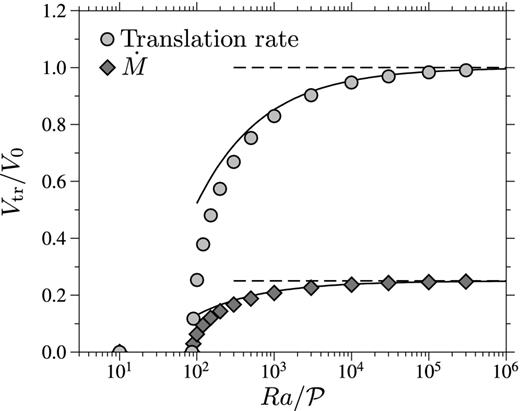
Translation rate and melt production, normalized by the low |$\mathcal {P}$| limit estimate given by eq. (107), as a function of |$Ra/\mathcal {P}$|⁠, for |$\mathcal {P}=10^{-2}$|⁠.

Fig. 9 shows the effect of increasing |$\mathcal {P}$| on the translation rate. In this figure, we have kept only simulations with |$Ra/\mathcal {P}$| larger than 105 to minimize the effect of the boundary layer, and further corrected the translation velocity with the boundary layer correction (eq. 115) found in Section 5.3, in order to isolate as much as possible the effect of |$\cal {P}$| on the translation mode. The |$\mathcal {O}(\mathcal {P})$| model developed in Section 5.2 (eq. 110, black line) agrees with the numerical simulations within 1 per cent for |$\mathcal {P}$| up to ∼3, but fails to explain the outputs of the numerical simulations when |$\mathcal {P}$| is larger, which indicates that higher order terms in |$\mathcal {P}$| become important.

Figure 9.

Translation rate (normalized by the low |$\mathcal {P}$| limit estimate given by eq. (107)) as a function of |$\mathcal {P}$|⁠, for different values of |$Ra/\mathcal {P}$|⁠. The thick black line show the prediction of the |$\mathcal {O}(\mathcal {P})$| model given by eq. (110).

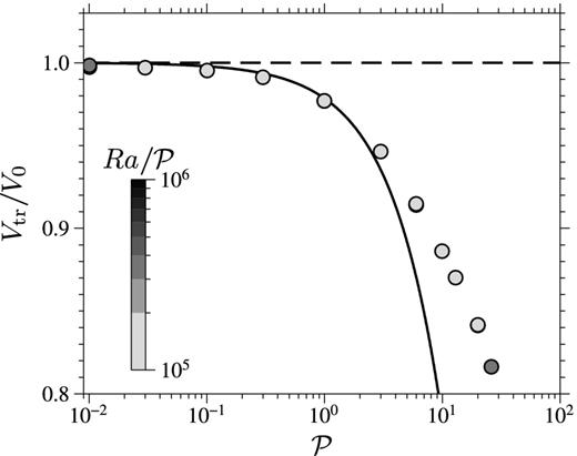
Overall, our analytical results (stability analysis and finite amplitude models) are in very good agreement with our numerical simulations when |$\mathcal {P}$| is small, which gives support to both our theory and to the validity of the numerical code.

6.3.2 Plume convection

If |$\mathcal {P}$| is large, the translation rate of the inner core becomes vanishingly small, but, as long as |$\mathcal {P}$| is finite, there is still a finite rate of melt production associated with the smaller scale topography arising from plume convection. A scaling for the melt production in the limit of large |$\mathcal {P}$| and large Ra can be derived from scaling relationship for infinite Prandtl number convection with impermeable boundaries. Parmentier & Sotin (2000) derived a set of scaling laws for high Rayleigh number internally heated thermal convection in a cartesian box, in the limit of infinite Prandtl number, but we found significant deviations from their model in our numerical simulations, which we ascribe to geometrical effects due to the spherical geometry. We therefore propose a set of new scaling laws for convection in a full sphere with internal heating.

Quantities of interest are the horizontal and vertical velocities u and w, the mean inner core potential temperature 〈Θ〉, the thermal boundary layer thickness δ, the thermal radius of the plumes a, the average plume spacing λh, and a length scale for radial variations of the velocity, which we note λr (see Fig. 10). The horizontal length scale λh is related to the number N of plumes per unit area by |$N\sim 1/\lambda _h^2$|⁠.

Figure 10.

A schematic of inner core plume convection, and definition of the length scales used in the scaling analysis. Streamlines of the flow are shown with thin arrowed grey lines.

Outputs of numerical simulations (〈Θ〉, δ, rms velocity Urms, rms radial velocity wrms, rms horizontal velocity urms, N) are shown in Figs 11(a)–(d) for Ra between 105 and 3 × 108. The boundary layer thickness δ is estimated as the ratio of the mean potential temperature in the inner core, 〈Θ〉, over the time and space averaged potential temperature gradient at the ICB: δ = −〈Θ〉/〈∂Θ/∂ricb. The time-averaged number N of plume per unit area is estimated by counting plumes on horizontal surfaces on typically 50 different snapshots. Both 〈Θ〉 and δ follow well-defined power law behaviours over this range of Ra. In contrast, the rms velocities and plume density N seem to indicate a change of behaviour at Ra close to 107. For Ra < 107, the vertical velocity increases faster than the horizontal velocity, while at larger Ra horizontal and vertical velocities increase with Ra at roughly the same rate.

Figure 11.

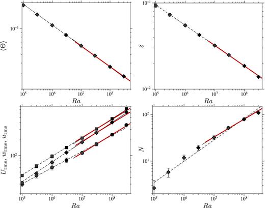
(a) Mean potential temperature 〈Θ〉 as a function of Ra for |$\mathcal {P}$| larger than 103. (b) Boundary layer thickness δ. (c) RMS velocity Urms (squares), rms vertical velocity wrms (diamonds), and rms horizontal velocity urms (circles). (d) Number of plumes N per unit surface. In figures (a) to (d), the thick red lines show the predictions of the scaling theory developed in Section 6.3.2 with β = −0.238. The dashed lines show the result of the individual least square inversion for each quantity for Ra ≥ 105.

We start our analysis by first noting that under statistically steady state conditions, the heat flux at the ICB must be equal, in a time-averaged sense, to the heat production within the inner core. In the thermal boundary layer, heat transport is dominated by conduction and the non-dimensional heat flux −〈∂Θ/∂ricb is equal to 〈Θ〉/δ. This must be in balance with the non-dimensional internal heat production. With our scaling, the mean potential temperature gradient should be equal to –2 on average, which implies that δ should be equal to 〈Θ〉/2. We can therefore write
\begin{equation} \delta = \frac{\langle \Theta \rangle }{2} \sim Ra^\beta , \end{equation}
(121)
where β is to be determined. We further assume that the thickness of the thermal boundary layer is set by a local stability criterion, that is, that the boundary layer Rayleigh number Raδ = (αρsgicbΘδ3)/(κη) is on average equal to some constant, which is equivalent to state that Raδ ∼ 1. Using non-dimensional 〈Θ〉 and δ, Raδ is related to the inner core Rayleigh number Ra by Raδ = Ra 〈Θ〉δ3. Given that 〈Θ〉 ∼ δ, this implies that Ra〈Θ〉δ3Ra δ4 ∼ 1, which gives β = −1/4.

The best fit of the numerical results (Figs 11a and b) gives 〈Θ〉 ∼ Ra−0.240 ± 0.005 and δ ∼ Ra−0.236 ± 0.003, in fair agreement with the predicted scaling. In Cartesian geometry, Parmentier & Sotin (2000) found β = −0.2448. Deschamps et al. (2012) found β = −0.238 for thermal convection in internally heated spherical shells.

The vertical plume velocity w is set by a balance between the buoyancy stress, ∼Ra〈Θ〉a, and the viscous stress, ∼wh. This gives
\begin{equation} \frac{w}{\lambda _h} \sim Ra\, \langle \Theta \rangle \, a. \end{equation}
(122)
In addition, the heat flux advected by the plumes, Nw〈Θ〉a2, must scale as the ICB heat flux, which, as already discussed above, must be ∼1. Since the number of plumes per unit area is |$N\sim 1/\lambda _h^2$|⁠, this gives
\begin{equation} 1 \sim \frac{a^2}{\lambda _h^2} \langle \Theta \rangle w. \end{equation}
(123)
The plume thermal radius a is related to the thermal boundary layer thickness through the conservation of mass, which when applied at the roots of the plumes implies that
\begin{equation} \delta u \sim a w. \end{equation}
(124)
Finally, conservation of mass in one convective cell implies that
\begin{equation} \frac{u}{\lambda _h} \sim \frac{w}{\lambda _r}. \end{equation}
(125)

This gives four eqs (122)–(125) for five unknowns (u, w, a, λh, λr). The system can be solved if additional assumptions are made on the scaling of λr. For high Pr, low Re convection, a natural choice would be to assume that radial variations of w occur at the scale of the radius of the inner core. This implies λr ∼ 1, and solving the system of eqs (122)–(125) with β = −0.24 gives aRa−0.14, uRa0.82, wRa0.72 and NRa−0.2, which agrees very poorly with the numerical results.

This poor agreement might be due to the spherical geometry. In a sphere, plumes converge towards each others while sinking, which is not the case in cartesian boxes, and is not a very significant effect in a spherical shell for which, like in Earth's mantle, the radius of the inner shell is a significant fraction of that of the outer shell. If Ra is large and the average plume spacing is small compared to the inner core radius, we might expect that the geometry of the convective cells becomes self-similar, with λr ∼ λh. With this assumption, we obtain
\begin{eqnarray} \lambda _h \sim \lambda _r & \sim Ra^{1+5\beta }, \end{eqnarray}
(126)
\begin{eqnarray} u\sim w & \sim Ra^{2+7\beta }, \end{eqnarray}
(127)
\begin{eqnarray} a \sim \delta \sim \langle \Theta \rangle & \sim Ra^\beta . \end{eqnarray}
(128)

Assuming a scaling of the form given by eqs (126)–(128), it is possible to inverse simultaneously all variables for β, the result of the inversion being β = −0.238 ± 0.003 (±1σ). The prediction of eqs (126)–(128) with this value of β are shown with red lines in Fig. 11a–d for Ra ≥ 107. They agree with the numerical outputs almost as well as individual inversions, which demonstrates the self-consistency of our scaling theory.

We can now derive a scaling for the rate of melt production |${\skew4 \dot{M}}$|⁠. The starting point is the continuity of the normal stress at the ICB, given by eq. (57). The local melting/solidification rate is given by the value of |$u_r-\dot{r}_\mathrm{ic}$| at the ICB (⁠|$u_r-\dot{r}_\mathrm{ic}>0$| means melting, and |$u_r-\dot{r}_\mathrm{ic}<0$| means solidification) which, according to eq. (57), can be written as
\begin{equation} u_r-\dot{r}_\mathrm{ic} = \mathcal {P}^{-1} \left( -2 \frac{\partial u_r}{\partial r} + \hat{p} \right). \end{equation}
(129)
As discussed above, we have
\begin{equation} \left.\frac{\partial u_r}{\partial r}\right|_\mathrm{icb} \sim \frac{w}{\lambda _r} \sim Ra^{1+2\beta }. \end{equation}
(130)
The dynamic pressure is given by the horizontal component of the Stokes equation,
\begin{equation} 0 = -\nabla _H \hat{p} + (\Delta u)_H \end{equation}
(131)
which implies that
\begin{equation} \hat{p} \sim \frac{u}{\lambda _h} \sim Ra^{1+2\beta }. \end{equation}
(132)
Both terms follow the same scaling, which implies that the global rate of melt production scales as
\begin{equation} {\skew4 \dot{M}} \sim Ra^{1+2\beta } \mathcal {P}^{-1}. \end{equation}
(133)
With β = −0.238 ± 0.003, we obtain |${\skew4 \dot{M}} \sim Ra^{0.524\pm 0.006} \mathcal {P}^{-1}$|⁠.

Fig. 12(b) shows |$\mathcal {P} {\skew4 \dot{M}}$| as a function of Ra, for |$\mathcal {P}\ge 10^3$| corresponding to the plume convection regime. There is an almost perfect collapse of the data points, which supports the fact that |${\skew4 \dot{M}} \propto \mathcal {P}$| in this regime. The kink in the curve at Ra ≃ 3 × 104 corresponds to the transition from steady convection to unsteady convection. Above this transition, the data points are well fitted by a power law of the form |${\skew4 \dot{M}} =a \mathcal {P}^{-1} Ra^{b}$|⁠. Least-square regression for Ra ≥ 3 × 105 gives a = 0.46 ± 0.04 and b = 0.554 ± 0.006, in reasonable agreement with the value found above. In dimensional terms, |${\skew4 \dot{M}} \simeq a ({\kappa }/{r_\mathrm{ic}}) \mathcal {P}^{-1}Ra^{b}$| and the mass flux of molten material is |$\rho _\mathrm{ic} {\skew4 \dot{M}} \simeq a {k}/({c_p r_\mathrm{ic}}) \mathcal {P}^{-1}Ra^{b}$|⁠.

Figure 12.

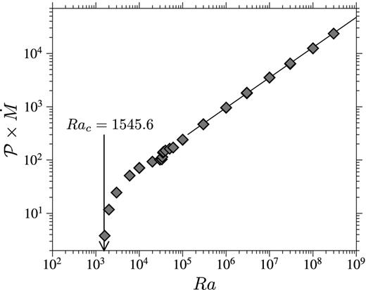
Rate of melt production (multiplied by |$\mathcal {P}$|⁠) as a function of Ra, for numerical simulations with |$\mathcal {P} \ge 10^3$|⁠. The value of the critical Rayleigh number as predicted by the linear stability analysis in the limit of infinite |$\mathcal {P}$| (eq. 89, Rac = 1545.6) is indicated by the arrow.

7 APPLICATION

7.1 Evolutive models

The analytical model for the translation mode and the scaling laws for large-|$\mathcal {P}$| convection derived in the previous sections strictly apply only to convection with ric and S constant. We therefore first check that our models correctly describe inner core convection when ric and S are time-dependent, by comparing their predictions with the outcome of numerical simulations with inner core growth and thermal history determined from the core energy balance.

To account for the inner core secular evolution, we follow the procedure explained in Deguen & Cardin (2011), where the growth of the inner core and its cooling rate are determined from the core energy balance. In this framework, a convenient way to write S(t) is
\begin{equation} S = \frac{\rho _s g^{\prime } \gamma T}{K_S} 3 \kappa \left[ f(r_\mathrm{ic})\,\mathcal {T}_\mathrm{ic}^{-1} - 1 \right], \end{equation}
(134)
where f (ric) is a decreasing order one function of ric defined in Deguen & Cardin (2011) (eq. 19, p. 1104), g′ = dg/dr, KS is the isentropic bulk modulus, γ the Grüneisen parameter, and
\begin{equation} \mathcal {T}_\mathrm{ic}=\left( \frac{{\rm d}T_s}{{\rm d}T_\mathrm{ad}}-1 \right)^{-1} \frac{\tau _\mathrm{ic}}{\tau _\kappa }, \end{equation}
(135)
where τic is the age of the inner core, |$\tau _\kappa =r_\mathrm{ic}^{*2}/(6\kappa )$| is the current inner core thermal diffusion time, and dTs/dTad is the ratio of the Clapeyron slope dTs/dP to the adiabat dTad/dP. The non-dimensional inner core age |$\mathcal {T}_\mathrm{ic}$| is a convenient indicator of the thermal state of the inner core, with |$\mathcal {T}_\mathrm{ic}<1$| implying unstable stratification for most of inner core history (see Deguen & Cardin 2011, fig. 3a). We give for reference in Table 2 the values of the age of the inner core τic corresponding to |$\mathcal {T}_\mathrm{ic}=0.8$|⁠, 1 and 1.2, for a thermal conductivity equal to 36, 79 and 150 W m−1 K−1. With the inner core growth history determined from the core energy balance and S(t) calculated from eq. (134), the evolution of Ra(t) and |$\mathcal {P}(t)$| can then be calculated.
Table 2.

Correspondence between τic and |$\mathcal {T}_\mathrm{ic}$| for three values of inner core thermal conductivity, assuming dTs/dTad = 1.65 ± 0.11 (Deguen & Cardin 2011).

k (W m−1 K−1)
3679150
0.81.18 ± 0.23 Gy0.54 ± 0.11 Gy0.28 ± 0.06 Gy
|${\mathcal {T}_\mathrm{ic}}=$|1.01.48 ± 0.29 Gy0.68 ± 0.13 Gy0.36 ± 0.07 Gy
1.21.77 ± 0.35 Gy0.81 ± 0.16 Gy0.43 ± 0.08 Gy
k (W m−1 K−1)
3679150
0.81.18 ± 0.23 Gy0.54 ± 0.11 Gy0.28 ± 0.06 Gy
|${\mathcal {T}_\mathrm{ic}}=$|1.01.48 ± 0.29 Gy0.68 ± 0.13 Gy0.36 ± 0.07 Gy
1.21.77 ± 0.35 Gy0.81 ± 0.16 Gy0.43 ± 0.08 Gy

Fig. 13(a) shows the trajectories of the inner core state in a |$Ra-\mathcal {P}$| space for four different scenarios, superimposed on a regime diagram for inner core thermal convection. According to eq. (6), the ICB phase change timescale scales as |$\tau _\phi \propto r_\mathrm{ic}^{-1}$|⁠, and therefore |$\mathcal {P}\propto r_\mathrm{ic}$| always increases during inner core history. In contrast, the evolution of Ra(t) is non monotonic, with the effect of the increasing inner core radius and gravity opposing the decrease with time of the effective heating rate S(t). Because S eventually becomes negative at some time in inner core history, Ra reaches a maximum before decreasing and eventually becoming negative, resulting in a bell shaped trajectory of the inner core in the |$Ra-\mathcal {P}$| space. The maximum in Ra may or may not have been reached yet, depending on the value of |$\mathcal {T}_\mathrm{ic}$|⁠.

Figure 13.

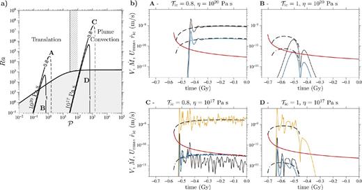
(a) Trajectories of the inner core state in a |$Ra-\mathcal {P}$| space, for the four cases A, B, C and D discussed in the text. The line annotations give the value of |$\mathcal {T}_\mathrm{ic}$| for each case. The dashed lines shows the future trajectory of the inner core. (b) Time evolution of V, |${\skew4 \dot{M}}$|⁠, Urms and |$\dot{r}_\mathrm{ic}$| for cases A to D. Red line: inner core growth rate |$\dot{r}_\mathrm{ic}$|⁠. Black line: translation rate V. Orange line-: rms velocity Urms. Blue line: dimensional melting rate |$(\kappa /r_\mathrm{ic}){\skew4 \dot{M}}$|⁠. Predictions for the rms velocity (or translation velocity in the translation regime) and melting rate |${\skew4 \dot{M}}$| are shown with thick dashed and dash-dotted lines, respectively. In the η = 1020 Pa s cases, the translation model (eq. 115) is used to predict V and |${\skew4 \dot{M}}$|⁠. In the η = 1017 Pa s case, the high-|$\mathcal {P}$| scaling is used for Urms and |${\skew4 \dot{M}}$|⁠. In the η = 1020 Pa s, |$\mathcal {T}_\mathrm{ic}=0.8$| and |$\mathcal {T}_\mathrm{ic}=1$| cases, the translation rate and the rms velocity are equal. For these simulations, the Rayleigh number was calculated assuming a thermal conductivity k = 79 W m−1 K−1 and a phase change timescale τϕ = 1000 yr. Values of other physical parameters used for these runs are summarized in Table 1.

The scenarios A--D shown in Fig. 13a have been chosen to illustrate four different possible dynamic histories of the inner core. In cases A and C, which have |$\mathcal {T}_\mathrm{ic}=0.8$|⁠, Ra remains positive and supercritical up to today, thus always permitting thermal convection. In cases B and D, which have |$\mathcal {T}_\mathrm{ic}=1$|⁠, Ra has reached a maximum early in inner core history, before decreasing below supercriticality, at which point convection is expected to stop. In these two cases, only an early convective episode is expected (Buffett 2009; Deguen & Cardin 2011). In cases A and B, which have η = 1020 Pa s, |$\mathcal {P}(t)$| is always smaller than the transitional |$\mathcal {P}_t$| and thermal convection therefore should be in the translation regime; Cases C and D, which have η = 1017 Pa s, have |$\mathcal {P}(t)>10^2>\mathcal {P}_t$| and thermal convection should be in the plume regime.

Fig. 13(b) shows outputs from numerical simulations corresponding to the inner core histories shown in Fig. 13(a). The numerical results are compared to the predictions for the rms velocity Urms (equal to the translation rate Vtr in the translation regime) and melting rate |${\skew4 \dot{M}}$| from the analytical translation model (eq. 116) and the large-|$\mathcal {P}$| scaling laws (eq. 133). The agreement is good in both the translation and plume convection regimes, except at the times of initiation and cessation of convection.

There is always a lag between when conditions become supercritical and when the amplitude of convective motions become significant, due to the finite growth rate of the instability. From eq. (88), the timescale for instability growth, τ = 1/σ, is approximately (in dimensional form)
\begin{equation} \tau \simeq 5 \frac{r_\mathrm{ic}^2}{\kappa } \left( \frac{Ra}{\mathcal {P}} - \left.\frac{Ra}{\mathcal {P}}\right|_c \right)^{-1} \simeq \left( \frac{r_\mathrm{ic}}{600\ {\rm km}} \right)^2 \displaystyle{\frac{90\ {\rm Myr}}{\frac{Ra}{\mathcal {P}}\left.\frac{Ra}{\mathcal {P}}\right|_c} - 1} \end{equation}
(136)
in the translation regime, and
\begin{equation} \tau \simeq 77 \frac{r_\mathrm{ic}^2}{\kappa } \left( Ra - Ra_c \right)^{-1} \simeq \left( \frac{r_\mathrm{ic}}{600\ {\rm km}} \right)^2 \frac{80\ {\rm Myr}}{{Ra}/{Ra}_c - 1} \end{equation}
(137)
in the large-|$\mathcal {P}$| regime. In both cases, the timescale for the growth of the instability will typically be a few tens of Myr, thus explaining the delayed initiation of convection seen in the numerical simulations.

In cases B and D, the flow occurring after t ≃ −0.46 Gy, at a time where the models predict no motion (because S < 0), corresponds to a slow relaxation of the thermal heterogeneities left behind by the convective episode.

Apart during the initiation and cessation periods of convection, the models developed for steady internal heating and constant inner core radius agree very well with the full numerical calculations, and can therefore be used to predict the dynamic state of the inner core and key quantities including rms velocity and melt production rate.

7.2 Melt production

Experiments by Alboussière et al. (2010) have shown that the development of a stably stratified layer above the ICB by inner core melting is controlled by the ratio ΦB of the buoyancy fluxes arising from the melting and freezing regions of the ICB. By using the analytical translation model and the scaling laws for plume convection developed in the last two sections, we can now estimate today's value of ΦB as a function of the state and physical properties of the inner core, and assess the likelihood of the origin of the F-layer by inner core melting.

With |${\skew4 \dot{M}}$| being the non-dimensional rate of melt production defined in eq. (117), the mean solidification rate is |$(\kappa /r_\mathrm{ic}){\skew4 \dot{M}} + \dot{r}_\mathrm{ic}$| from conservation of mass. The buoyancy flux associated with the release of dense fluid by melting can be written as |$- \Delta \rho _\chi \, g_\mathrm{icb} (\kappa /r_\mathrm{ic}) {\skew4 \dot{M}}$|⁠, while the buoyancy flux associated with the solidification is |$\Delta \rho _\chi \, g_\mathrm{icb} [(\kappa /r_\mathrm{ic}){\skew4 \dot{M}} + \dot{r}_\mathrm{ic}]$|⁠, where Δρχ is the fraction of the ICB density jump due to the compositional difference. According to Alboussière et al. (2010)'s experiments, a stratified layer is expected to form above the ICB if the magnitude of the buoyancy flux associated with melting is more than 80 per cent of the buoyancy flux associated with solidification, that is, if
\begin{equation} \Phi _B = \frac{ \Delta \rho _\chi \, g_\mathrm{icb} (\kappa /r_\mathrm{ic}) {\skew4 \dot{M}}}{\Delta \rho _\chi \, g_\mathrm{icb} [(\kappa /r_\mathrm{ic}){\skew4 \dot{M}} + \dot{r}_\mathrm{ic}]}= \frac{ {\skew4 \dot{M}}}{{\skew4 \dot{M}} + \dot{r}_\mathrm{ic}\, r_\mathrm{ic}/\kappa } > 0.8, \end{equation}
(138)
which requires that
\begin{equation} \frac{\kappa }{r_\mathrm{ic}}{\skew4 \dot{M}} > 4\, \dot{r}_\mathrm{ic}. \end{equation}
(139)
In the translation regime, in which |${\skew4 \dot{M}} = V/4$|⁠, this requires that the rate of translation is at least 16 times larger than the mean solidification rate of the inner core.
The current inner core growth rate can be expressed as
\begin{equation} \dot{r}_\mathrm{ic} = \frac{3\kappa }{r_\mathrm{ic}} \frac{f(r_\mathrm{ic}) }{\left(\frac{{\rm d}T_s}{{\rm d}T_\mathrm{ad}}-1\right)\mathcal {T}_\mathrm{ic}} \end{equation}
(140)
where the function f (ric) ≃ 0.8 at the current inner core radius (Deguen & Cardin 2011). Using this expression, the buoyancy ratio ΦB is
\begin{equation} \Phi _B = 1 - \left[ 1 + \left(\frac{{\rm d}T_s}{{\rm d}T_\mathrm{ad}} -1 \right) \frac{\mathcal {T}_\mathrm{ic}}{3 f(r_\mathrm{ic})} \frac{V}{4} \right]^{-1} \end{equation}
(141)
in the translation regime, with the translation velocity V given by eq. (115), and
\begin{equation} \Phi _B = 1 - \left[ 1 + \left(\frac{{\rm d}T_s}{{\rm d}T_\mathrm{ad}} -1 \right) \frac{\mathcal {T}_\mathrm{ic}}{3 f(r_\mathrm{ic})} a \mathcal {P}^{-1} Ra^b \right]^{-1} \end{equation}
(142)
in the high-|$\mathcal {P}$| regime.

7.3 Today's inner core regime and rate of melt production

The inner core dynamic regime depends mostly on the value of its non-dimensional age |$\mathcal {T}_\mathrm{ic}$| and of |$\mathcal {P}$|⁠, both parameters being very poorly constrained. The value of |$\mathcal {T}_\mathrm{ic}$| dictates whether the inner core has a stable or unstable temperature profile, and the parameter |$\mathcal {P}$| determines the convection regime if the inner core is unstable against thermal convection. Other parameters have a comparatively small influence on the inner core dynamics, and on the value of ΦB. With this idea in mind, it is useful to rewrite the Rayleigh number as a function of |$\mathcal {P}$| and |$\mathcal {T}_\mathrm{ic}$|⁠:
\begin{eqnarray} Ra &=& \displaystyle\frac{\alpha \rho _s g_\mathrm{icb} S r_\mathrm{ic}^5}{6 \kappa ^2 \eta } \nonumber \\ &=& \displaystyle\mathcal {A} \left[ f(r_\mathrm{ic})\,\mathcal {T}_\mathrm{ic}^{-1} - 1 \right] \mathcal {P},\quad {\rm with}\ \mathcal {A}= \frac{\alpha ^2 \rho _s^2\, g_\mathrm{icb} r_\mathrm{ic}^3 T}{2\, k\, \Delta \rho \, \tau _\phi }. \end{eqnarray}
(143)
The exact value of the pre-factor |$\cal {A}$| affects the value of ΦB, but not the inner core regime (stably stratified inner core, translation, or plume convection) which is determined by |$\mathcal {P}$| and |$\mathcal {T}_\mathrm{ic}$|⁠. The uncertainty on |$\mathcal {A}$| comes mostly from the uncertainty on τϕ, which is difficult to estimate without a better understanding of the dynamics of the F-layer. If |$\mathcal {P}$| and |$\mathcal {T}_\mathrm{ic}$| are kept constants, changing |$\mathcal {A}$| by an order of magnitude would change the translation velocity and melting rates (in both regimes) by a factor of ∼3. Fig. 14 shows ΦB as a function of |$\mathcal {T}_\mathrm{ic}$| and |$\mathcal {P}$|⁠, calculated from eqs (141) and (142) with Ra given by eq. (143) and |$\mathcal {A}=3\times 10^5$| (corresponding to parameters values given in Table 1). Fig. 14 serves both as a regime diagram for the inner core, and as a predictive map for ΦB and the likelihood of the development of a stratified layer at the base of the outer core.
Figure 14.

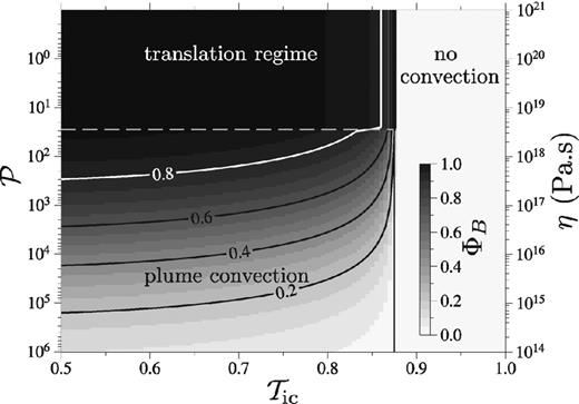
Inner core regime diagram and map of the buoyancy ratio ΦB, as functions of |$\mathcal {P}$| and |$\mathcal {T}_\mathrm{ic}$|⁠. The corresponding values of η assuming τϕ = 1000 yr are given on the right hand size vertical axis. According to Alboussière et al. (2010)'s experiments, inner core melting can produce a stably stratified layer at the base of the outer core if ΦB > 0.8 (white contour).

The inner core has currently an unstable thermal profile only if |$\mathcal {T}_\mathrm{ic}$| is smaller than ≃0.87. The mode of thermal convection then depends on |$\mathcal {P}$|⁠, with the translation regime (small |$\mathcal {P}$|⁠) being the most efficient at producing melt. Plume convection generates less melt, but the rate of melt production still remains significant as long as |$\mathcal {P}$| is not too large (η not too small). The critical value of ΦB = 0.8 (white contour in Fig. 14) suggested by the experiments of Alboussière et al. (2010) is almost always reached in the translation regime, but only in a small part of the parameter space in the plume convection regime.

8 COMPOSITIONAL EFFECTS

We have so far left aside the possible effects of the compositional evolution of the outer and inner core on the inner core dynamics. We will argue here that the development of an iron rich layer above the inner core can have a possibly important positive feedback on inner core convection: irrespectively of the exact mechanism at the origin of the F-layer (Gubbins et al.2008, 2011; Alboussière et al.2010), its interpretation as an iron rich layer implies a decrease with time of light elements concentration in the liquid just above the ICB. This in turn implies that the newly crystallized solid is increasingly depleted in light elements, and intrinsically denser, which may drive compositional convection in the inner core. The reciprocal coupling between the inner core and the F-layer may create a positive feedback loop which can make the system (inner core + F-layer) unstable. The mechanism releases more gravitational energy than purely radial inner core growth with no melting, and should therefore be energetically favored.

We note c s and cl the light element concentration in the inner and outer core, respectively, |$c_\mathrm{icb}^{s,l}$| their values at the ICB, and |$\dot{c}_\mathrm{icb}^{s,l} = {\rm d} c_\mathrm{icb}^{s,l}/{\rm d}t$| their time derivatives at the ICB. The concentration in the liquid and solid sides of the ICB are linked by the partition coefficient k, |$c_\mathrm{icb}^s = k\,c_\mathrm{icb}^l$|⁠. Introducing |$\tilde{c} = c - c_\mathrm{icb}^s$|⁠, the equation of transport of light element can be written as
\begin{equation} \frac{{\rm D} \tilde{c}}{{\rm D}t} = \kappa _c \nabla ^2 \tilde{c} + S_c, \quad \tilde{c}(r_\mathrm{ic})=0, \end{equation}
(144)
with
\begin{equation} S_c = - \dot{c}_\mathrm{icb}^s = - k\, \dot{c}_\mathrm{icb}^l - c_\mathrm{icb}^l \frac{{\rm d} k}{{\rm d}t}, \end{equation}
(145)
which is an exact analogue of the potential temperature transport eq. (29). The only—but important—difference is that the source term Sc is a dynamic quantity which depends on the convective state of the inner core and on the dynamics of the F-layer rather than being externally imposed like the effective heating rate S, which means that the dynamics of the inner core and F-layer must be considered simultaneously.
In general, the fact that the thermal and compositional diffusivities are different can be of importance, and would lead to double-diffusive type convection. However this is not the case in the translation regime, for which diffusion does not play any role as long as the translation rate is large enough (i.e. if the Péclet number Pe = Vric/κ ≫ 1). Thanks to the potential temperature/composition analogy noted above, the translation model developed for thermal convection can be extended to include compositional effects, the translation rate being given by
\begin{equation} V = \left[ \frac{1}{5}\frac{\rho _s}{\Delta \rho } \frac{(\alpha S + \alpha _c\, S_c)}{\tau _\phi } \right]^{1/2} r_\mathrm{ic} \end{equation}
(146)
when compositional effects are accounted for. We therefore need to compare the magnitudes of αS and |$\alpha _c\,S_c=-\alpha _c\, k\, \dot{c}_\mathrm{icb}^l-\alpha _c\,c_\mathrm{icb}^l\, {\rm d}k/{\rm d}t$|⁠. Assuming (Gubbins et al.2008) that the light element concentration at the base of the F-layer is currently about twice smaller than the outer core mean concentration, coc ≃ 5 wt. per cent, we obtain |$\dot{c}_\mathrm{icb}^l\sim -0.5\, c_\mathrm{oc}/\tau _\mathrm{ic}\sim -10^{-18}$| wt. per cent s−1 with τic ∼ 1 Gy. With αc ≃ 1, this gives |$-\alpha _c\, k\, \dot{c}_\mathrm{icb}^l \sim 10^{-19}$| s−1 if k ≃ 0.1 and |$-\alpha _c\, k\, \dot{c}_\mathrm{icb}^l \sim 10^{-20}$| s−1 if k ≃ 0.01, which is similar or larger than the thermal contribution α S ∼ 10−5 × 10−15 ∼ 10−20 s−1. The term |$-\alpha _c\,c_\mathrm{icb}^l\, {\rm d}k/{\rm d}t$| might be positive as well. According to calculations by Gubbins et al. (2013), the variation with temperature of the partitioning behaviour of Oxygen can produce an unstable compositional gradient. As discussed in Alboussière et al. (2010) and Deguen & Cardin (2011), the effective partition coefficient may also decrease with time because of dynamic reasons (the efficiency of melt expulsion from the inner core increases with inner core size), which would also imply that this term is positive.

There is an additional feedback, this time negative, which comes from the effect of composition on the solidification temperature, which increases with decreasing light element concentration. The decreasing light element concentration at the base of the F-layer implies that the ICB temperature decreases with time at a slower rate than if the composition is fixed, which results in a smaller effective heating rate S (eq. 30). For a fixed inner core growth rate, this decreases the ICB cooling rate by an amount equal to |$-m_c \, \dot{c}_\mathrm{icb}^l$|⁠, where mc = ∂Ts/∂c ∼ −104 K (Alfè et al.2002) is the liquidus slope at the inner core boundary pressure and composition. This adds a term |$-\alpha \, m_c \, \dot{c}_\mathrm{icb}^l$| in eq. (146). If only one light element is considered, the ratio of the stabilizing term |$\alpha \, m_c \, \dot{c}_\mathrm{icb}^l$| over the destabilizing term |$-\alpha _c\, k\, \dot{c}_\mathrm{icb}^l$| is ∼α mc/(αck) ∼ −0.1/k. The two terms are of the same order of magnitude if k ∼ 0.1, but the negative feedback dominates if k is smaller.

The above estimates are clearly uncertain, and a dynamic model of the F-layer will be required for assessing in a self-consistent way the effect of the development of the F-layer on inner core convection. There are several feedbacks of the formation of an F-layer on inner core convection, either positive or negative, and it is not clear yet whether the net effect would be stabilizing or destabilizing. Still, it does suggest that the effect could be important, and worth considering in more details.

9 SUMMARY AND CONCLUSIONS

Inner core translation can potentially explain a significant part of the inner core structure, but its existence depends critically on the value of a number of poorly constrained parameters. In this paper, we have studied in details the conditions for and dynamics of inner core thermal convection when melting and solidification at the ICB are allowed. We summarize here the main results and implications of our work:

  • If the inner core is convectively unstable, linear stability analysis (Section 4), asymptotic calculations (Section 5), and direct numerical simulations (Section 6) consistently show that the convection regime depends mostly on a non-dimensional number, the ‘phase change number’ |$\mathcal {P}$|⁠, characterizing the resistance to phase change (eq. 58). The convective translation mode dominates only if |$\mathcal {P}<29$|⁠, which requires that the inner core viscosity is larger than a critical value estimated to be ∼3 × 1018 Pa s. If |$\mathcal {P}$| is larger (smaller viscosity), melting and solidification at the ICB have only a small dynamic effect, and convection takes the usual form of low Prandtl number internally heated convection, with a one-cell axisymmetric mode at the onset, and chaotic plume convection if the Rayleigh number is large.

  • With published estimates of the inner core viscosity ranging from 1011 to 1022 Pa s (Yoshida et al.1996; Buffett 1997; Van Orman 2004; Mound & Buffett 2006; Koot & Dumberry 2011; Reaman et al.2011, 2012), the question of which mode would be preferred is open (although we note that the latest estimate from mineral physics, 1020–1022 Pa s (Reaman et al.2012), would put the inner core, if unstably stratified, well within the translation regime).

  • The two convection regimes have been characterized in details in Sections 4–7; a summary of theoretical results and scaling laws for useful dynamic quantities (rms velocity, rate of melt production, mean potential temperature, number of plumes per unit area, and strain rate) is given in Table 3. If the inner core is unstably stratified, the rate of melt production predicted by our models is always large enough to produce an iron-rich layer at the base of the outer, according to Alboussière et al. (2010)'s experiments, if the inner core is in the translation regime (Fig. 14). In the plume convection regime, the rate of melt production can still be significant if |$\mathcal {P}$| is not too large (η not too small).

  • Being driven by buoyancy, a prerequisite for the existence of convective translation is that an unstable density profile is maintained within the inner core. Thermal convection requires that a superadiabatic temperature profile is maintained with the inner core, which is highly dependent on the core thermal history and inner core thermal conductivity. With k = 36 W m−1 K−1 as proposed by Stacey & Davis (2008), this would be very likely (Buffett 2009; Deguen & Cardin 2011). However, several independent groups (Sha & Cohen 2011; de Koker et al.2012; Pozzo et al.2012) have recently argued for a much higher core thermal conductivity, around 150 W m−1 K−1 or higher. This would make thermal convection in the inner core, whether in the translation mode or in the plume convection mode, impossible unless the inner core is very young (≃300 Myr or less, which would require a probably excessively high CMB heat flux).

  • Compositional convection might be a viable alternative to thermal convection, either because the temperature dependency of the light elements partitioning behaviour can produce an unstable compositional profile (Gubbins et al.2013), or because of a possibly positive feedback of the development of the F-layer on inner core convection. As proposed in Section 8, the formation of an iron-rich layer at the base of the outer core over the history of the inner core implies that the inner core crystallizes from a source which is increasingly depleted in light elements. This in turn implies that the newly crystallized solid is increasingly depleted in light element, which results in an unstable density profile. Whether this positive feedback is strong enough to overcome the stabilizing effect of a possibly subadiabatic temperature profile depends on the dynamics of the F-layer, and further work is needed to test this idea.

Table 3.

Summary of theoretical results and scaling laws for the translation (⁠|$\mathcal {P} \lesssim 29$|⁠) and plume convection (⁠|$\mathcal {P} \gg 29$|⁠) regimes. In the plume convection regime, the value of β obtained by fitting the numerical outputs to our scaling theory is β = −0.238 ± 0.003.

Translation regimePlume convection regime
|$\mathcal {P} \lesssim 29$||$\mathcal {P} \gg 29$|
Onset|$(\frac{Ra}{\mathcal {P}})_{c} = \frac{175}{2}$|Rac = 1545.6
Velocity scaling , V or Urms|$\frac{\kappa }{r_\mathrm{ic}} \sqrt{\frac{6}{5}\frac{Ra}{\mathcal {P}}}$||$0.96 \frac{\kappa }{r_\mathrm{ic}} Ra^{2+7\beta }$|
Rate of melt production, |${\skew4 \dot{M}}$||$\frac{1}{4}\frac{\kappa }{r_\mathrm{ic}} \sqrt{\frac{6}{5}\frac{Ra}{\mathcal {P}}}$||$0.46\frac{\kappa }{r_\mathrm{ic}} Ra^{1+2\beta } \mathcal {P}^{-1}$|
〈Θ〉|$\frac{S r_\mathrm{ic}^2}{\kappa } (\frac{10}{3}\frac{\mathcal {P}}{Ra})^{1/2}$||$2.9 \frac{S r_\mathrm{ic}^2}{\kappa } Ra^\beta$|
Number of plumes per unit area, N|$\frac{0.07}{r_\mathrm{ic}^2} Ra^{-2-10\beta }$|
Strain rate |$\dot{\epsilon }\sim \frac{U_\mathrm{rms}}{\lambda } \sim \sqrt{N} U_\mathrm{rms}$||$0.25 \frac{\kappa }{r_\mathrm{ic}^2} Ra^{1+2\beta }$|

|$Ra = \frac{\alpha \rho _s g_\mathrm{icb} S r_\mathrm{ic}^5 }{6 \kappa ^2 \eta }$|⁠, |${\cal {P}} = \frac{\Delta \rho \, g_\mathrm{icb} \, r_\mathrm{ic} \, \tau _\phi }{\eta }$|⁠.

We would like to thank the two anonymous referees for many helpful comments and suggestions. All the computations presented in this paper were performed at the Service Commun de Calcul Intensif de l’Observatoire de Grenoble (SCCI). RD was supported by grant EAR-0909622 and Frontiers in Earth System Dynamics grant EAR-1135382 from the National Science Foundation. TA was supported by the ANR (Agence National de la Recherche) within the CrysCore project ANR-08-BLAN-0234-01, and by the program PNP of INSU/CNRS. PC was supported by the program PNP of INSU/CNRS.

REFERENCES

Abramovich
M.
Stegun
I.
Handbook of Mathematical Functions
1965
Washington, DC
US Government Printing Office
 
Fourth Printing. Applied Math. Ser. 55
Alboussière
T.
Ricard
Y.
Reflections on dissipation associated with thermal convection
J. Fluid Mech.
2013
, vol. 
725
  
doi:10.1017/jfm.2013.241
Alboussière
T.
Deguen
R.
Melzani
M.
Melting induced stratification above the Earth's inner core due to convective translation
Nature
2010
, vol. 
466
 (pg. 
744
-
747
)
Alfè
D.
Gillan
M.J.
Price
G.D.
Ab initio chemical potentials of solid and liquid solutions and the chemistry of the Earth's core
J. Chem. Phys.
2002
, vol. 
116
 (pg. 
7127
-
7136
)
Anderson
O.L.
Wenk Duba
A.
Experimental melting curve of iron revisited
J. geophys. Res.
1997
, vol. 
102
 (pg. 
22 659
-
22 670
)
Anufriev
A.
Jones
C.
Soward
A.
The Boussinesq and anelastic liquid approximations for convection in the Earth's core
Phys. Earth planet. Inter.
2005
, vol. 
12
 
3
(pg. 
163
-
190
)
Aubert
J.
Flow throughout the Earth's core inverted from geomagnetic observations and numerical dynamo models
Geophys. J. Int.
2013
, vol. 
192
 
2
(pg. 
537
-
556
)
Bergman
M.
Lewis
D.
Myint
I.
Slivka
L.
Karato
S.
Abreu
A.
Grain growth and loss of texture during annealing of alloys, and the translation of Earth's inner core
Geophys. Res. Lett.
2010
, vol. 
37
 
22
pg. 
L22313
  
doi:10.1029/2010GL045103
Buffett
B.
Onset and orientation of convection in the inner core
Geophys. J. Int.
2009
, vol. 
179
 (pg. 
711
-
719
)
Buffett
B.A.
Geodynamics estimates of the viscosity of the Earth's inner core
Nature
1997
, vol. 
388
 (pg. 
571
-
573
)
Buffett
B.A.
Wenk
H.-R.
Texturing of the Earth's inner core by Maxwell stresses
Nature
2001
, vol. 
413
 (pg. 
60
-
63
)
Chandrasekhar
S.
Hydrodynamic and Hydromagnetic Stability
1961
Clarendon, Oxford
International Series of Monographs on Physics
Christensen
U.
Aubert
J.
Scaling properties of convection-driven dynamos in rotating spherical shells and application to planetary magnetic fields
Geophys. J. Int.
2006
, vol. 
166
 
1
(pg. 
97
-
114
)
Cottaar
S.
Buffett
B.
Convection in the Earth's inner core
Phys. Earth planet. Inter.
2012
, vol. 
198-199
 (pg. 
67
-
78
)
Davies
C.J.
Silva
L.
Mound
J.
On the influence of a translating inner core in models of outer core convection
Phys. Earth planet. Inter.
2013
, vol. 
214
 pg. 
104–114
 
de Koker
N.
Steinle-Neumann
G.
Vlcek
V.
Electrical resistivity and thermal conductivity of liquid fe alloys at high p and t, and heat flux in earth's core
Proc. Natl. Acad. Sci.
2012
, vol. 
109
 
11
(pg. 
4070
-
4073
)
Deguen
R.
Cardin
P.
Thermo-chemical convection in Earth's inner core
Geophys. J. Int.
2011
, vol. 
187
 (pg. 
1101
-
1118
)
Deguen
R.
Cardin
P.
Merkel
S.
Lebensohn
R.
Texturing in Earth's inner core due to preferential growth in its equatorial belt
Phys. Earth planet. Inter.
2011
, vol. 
188
 (pg. 
173
-
184
)
Deschamps
F.
Yao
C.
Tackley
P.J.
Sanchez-Valle
C.
High rayleigh number thermal convection in volumetrically heated spherical shells
J. geophys. Res.-Solid Earth
2012
, vol. 
117
 pg. 
E09006
  
doi:10.1029/2012JE004090
Dziewonski
A.M.
Anderson
D.L.
Preliminary reference Earth model
Phys. Earth planet. Inter.
1981
, vol. 
25
 (pg. 
297
-
356
)
Forte
A.M.
Peltier
W.R.
Plate tectonics and aspherical Earth structure: the importance of poloidal-toroidal coupling
J. geophys. Res.
1987
, vol. 
92
 (pg. 
3645
-
3679
)
Geballe
Z.M.
Lasbleis
M.
Cormier
V.F.
Day
E.A.
Sharp hemisphere boundaries in a translating inner core
Geophys. Res. Lett.
2013
, vol. 
40
  
doi:10.1002/grl.50372
Gillet
N.
Pais
M.A.
Jault
D.
Ensemble inversion of time-dependent core flow models
Geophys. J. Int.
2009
, vol. 
10
 pg. 
Q06004
  
doi:10.1029/2008GC002290
Gubbins
D.
Masters
G.
Nimmo
F.
A thermochemical boundary layer at the base of Earth's outer core and independent estimate of core heat flux
Geophys. J. Int.
2008
, vol. 
174
 (pg. 
1007
-
1018
)
Gubbins
D.
Sreenivasan
B.
Mound
J.
Rost
S.
Melting of the Earth's inner core
Nature
2011
, vol. 
473
 
7347
(pg. 
361
-
363
)
Gubbins
D.
Alfè
D.
Davies
D.
Compositional instability of Earth's solid inner core
Geophys. Res. Lett.
2013
, vol. 
40
 
1–5
(pg. 
361
-
363
)
Irving
J.
Deuss
A.
Woodhouse
J.
Normal mode coupling due to hemispherical anisotropic structure in Earth's inner core
Geophys. J. Int.
2009
, vol. 
178
 
2
(pg. 
962
-
975
)
Jeanloz
R.
Wenk
H.-R.
Convection and anisotropy of the inner core
Geophys. Res. Lett.
1988
, vol. 
15
 (pg. 
72
-
75
)
Karato
S.-I.
Seismic anisotropy of the Earth's inner core resulting from flow induced by Maxwell stresses
Nature
1999
, vol. 
402
 (pg. 
871
-
873
)
Koot
L.
Dumberry
M.
Viscosity of the earth's inner core: constraints from nutation observations
Earth planet. Sci. Lett.
2011
, vol. 
308
 
3–4
(pg. 
343
-
349
)
Mizzon
H.
Monnereau
M.
Implications of the lopsided growth for the viscosity of Earth's inner core
Earth planet. Sci. Lett.
2013
, vol. 
361
 (pg. 
391
-
401
)
Monnereau
M.
Calvet
M.
Margerin
L.
Souriau
A.
Lopsided growth of Earth's inner core
Science
2010
, vol. 
328
 (pg. 
1014
-
1017
)
Mound
J.E.
Buffett
B.A.
Detection of a gravitational oscillation in length-of-day
Earth planet. Sci. Lett.
2006
, vol. 
243
 (pg. 
383
-
389
)
Niu
F.L.
Wen
L.X.
Hemispherical variations in seismic velocity at the top of the Earth's inner core
Nature
2001
, vol. 
410
 (pg. 
1081
-
1084
)
Pais
A.
Jault
D.
Quasi-geostrophic flows responsible for the secular variation of the Earth's magnetic field
Geophys. J. Int.
2008
, vol. 
173
 (pg. 
421
-
443
)
Parmentier
E.M.
Sotin
C.
Three-dimensional numerical experiments on thermal convection in a very viscous fluid: implications for the dynamics of a thermal boundary layer at high Rayleigh number
Phys. Fluids
2000
, vol. 
12
 (pg. 
609
-
617
)
Poirier
J.-P.
Physical properties of the Earth's core
C.R. Acad. Sci. Paris
1994
, vol. 
318
 (pg. 
341
-
350
)
Pozzo
M.
Davies
C.
Gubbins
D.
Alfè
D.
Thermal and electrical conductivity of iron at Earth's core conditions
Nature
2012
, vol. 
485
 (pg. 
355
-
358
)
Reaman
D.
Colijn
H.
Yang
F.
Hauser
A.
Panero
W.
Interdiffusion of Earth's core materials to 65 GPa and 2200K
Earth planet. Sci. Lett.
2012
, vol. 
349
 (pg. 
8
-
14
)
Reaman
D.M.
Daehn
G.S.
Panero
W.R.
Predictive mechanism for anisotropy development in the Earth's inner core
Earth planet. Sci. Lett.
2011
, vol. 
312
 
3–4
(pg. 
437
-
442
)
Ribe
N.M.
Gerald
S.
Bercovici
D.
Analytical approaches to mantle dynamics
Treatise on Geophysics
2007
New York
Elsevier
(pg. 
167
-
226
)
Schubert
G.
Turcotte
D.
Olson
P.
Mantle Convection in the Earth and Planets
2001
Cambridge, UK
Cambridge University Press
Sha
X.
Cohen
R.
First-principles studies of electrical resistivity of iron under pressure
J. Phys.: Conden. Matter
2011
, vol. 
23
 pg. 
075401
  
doi:10.1088/0953-8984/23/7/075401
Sneddon
I.
On some infinite series involving the zeros of bessel functions of the first kind
Proceedings of the Glasgow Mathematical Association
1960
Cambridge, UK
Cambridge University Press
(pg. 
144
-
156
Vol 4
Souriau
A.
Poupinet
G.
The velocity profile at the base of the liquid core from PKP(BC+Cdiff) data: an argument in favor of radial inhomogeneity
Geophys. Res. Lett.
1991
, vol. 
18
 (pg. 
2023
-
2026
)
Sreenivasan
B.
Gubbins
D.
On mantle-induced heat flow variations at the inner core boundary
Phys. Earth planet. Inter
2011
, vol. 
187
 (pg. 
336
-
341
)
Stacey
F.
Loper
D.
A revised estimate of the conductivity of iron alloy at high pressure and implications for the core energy balance
Phys. Earth planet. Inter.
2007
, vol. 
161
 (pg. 
13
-
18
)
Stacey
F.D.
Anderson
O.L.
Electrical and thermal conductivities of Fe-Ni-Si alloy under core conditions
Phys. Earth planet. Inter.
2001
, vol. 
124
 (pg. 
153
-
162
)
Stacey
F.D.
Davis
P.M.
Physics of the Earth
2008
Cambridge, UK
Cambridge University Press
Stevenson
D.
Limits on lateral density and velocity variations in the Earth's outer core
Geophys. J. R. astr. Soc.
1987
, vol. 
88
 
1
(pg. 
311
-
319
)
Sumita
I.
Yoshida
S.
Hamano
Y.
Kumazawa
M.
Yukutake
T.
A model for the structural evolution of the Earth's core and its relation to the observations
The Earth's Central Part: Its Structure and Dynamics
1995
Tokyo
Terra Scientific Publishing Company (Terrapub)
(pg. 
231
-
260
)
Tanaka
S.
Depth extent of hemispherical inner core from pkp (df) and pkp (cdiff) for equatorial paths
Phys. Earth planet. Inter
2012
, vol. 
210–211
 (pg. 
50
-
62
)
Tanaka
S.
Hamaguchi
H.
Degree one heterogeneity and hemispherical variation of anisotropy in the inner core from PKP(BC)-PKP(DF) times
J. geophys. Res.
1997
, vol. 
102
 (pg. 
2925
-
2938
)
Tritton
D.
Physical Fluid Dynamics
1988
Oxford
Clarendon Press
Van Orman
J.A.
On the viscosity and creep mechanism of Earth's inner core
Geophys. Res. Lett.
2004
, vol. 
31
 pg. 
L20606
  
doi:10.1029/2004GL021209
Vočadlo
L.
Ab initio calculations of the elasticity of iron and iron alloys at inner core conditions: evidence for a partially molten inner core?
Earth planet. Sci. Lett.
2007
, vol. 
254
 (pg. 
227
-
232
)
Weber
P.
Machetel
P.
Convection within the inner-core and thermal implications
Geophys. Res. Lett.
1992
, vol. 
19
 (pg. 
2107
-
2110
)
Yoshida
S.
Sumita
I.
Kumazawa
M.
Growth model of the inner core coupled with the outer core dynamics and the resulting elastic anisotropy
J. geophys. Res.
1996
, vol. 
101
 (pg. 
28 085
-
28 104
)

APPENDIX A: LINEAR STABILITY ANALYSIS

We investigate here the linear stability of the system of equations describing thermal convection in the inner core with phase change at the ICB, as derived in Section 3. The calculation given here is a generalization of the linear stability analysis of thermal convection in an internally heated sphere given by Chandrasekhar (1961).

We assume constant Ra and |$\mathcal {P}$|⁠. The basic state of the problem is then
\begin{equation} \bar{\Theta }= 1 - r^2, \end{equation}
(A1)
\begin{equation} \bar{ \mathbf {u}} = \mathbf {0}, \end{equation}
(A2)
which is the steady conductive solution of the system of equation developed in Section 3. We investigate the stability of this conductive state against infinitesimal perturbations of the temperature and velocity fields. The temperature field is written as the sum of the conductive temperature profile given by eq. (A1) and infinitesimal disturbances |$\tilde{\Theta }$|⁠, |$\Theta (r,\theta ,\phi ,t) = \bar{\Theta }(r) + \tilde{\Theta }(r,\theta ,\phi ,t)$|⁠. The velocity field perturbation is noted |$\tilde{\mathbf {u}}(r,\theta ,\phi ,t)$|⁠, and has an associated poloidal scalar |${\skew4 \tilde{P}}(r,\theta ,\phi ,t)$|⁠. We expand the temperature and poloidal disturbances in spherical harmonics,
\begin{equation} \tilde{\Theta } = \sum _{l=0}^\infty \sum _{m=-l}^l \tilde{t}_l^m(r) Y_l^m(\theta ,\phi )\, \mathrm{e}^{\sigma _l t}, \end{equation}
(A3)
\begin{equation} {\skew4 \tilde{P}} =\sum _{l=1}^\infty \sum _{m=-l}^l {\skew4 \tilde{p}}_l^m(r) Y_l^m(\theta ,\phi )\, \mathrm{e}^{\sigma _l t}, \end{equation}
(A4)
where σl is the growth rate of the degree l perturbations.
The only non-linear term in the system of equations is the advection of heat u · ∇T, which is linearized as
\begin{equation} \tilde{u}_r \frac{\partial \bar{\Theta }}{\partial r} = -2 r \tilde{u}_r = - 2 L^2 {\skew4 \tilde{P}} . \end{equation}
(A5)
The resulting linearized transport equation for the potential temperature disturbance is
\begin{equation} \frac{\partial \tilde{\Theta }}{\partial t} = {\nabla }^2 \tilde{\Theta }+ 2 L^2 {\skew4 \tilde{P}} + 6. \end{equation}
(A6)
Using the decompositions (A3) and (A4), the linearized system of equations is then, for l ≥ 1,
\begin{equation} Ra\, \tilde{t}_l^m = \mathcal {D}_l^2 {\skew4 \tilde{p}}_l^m, \end{equation}
(A7)
\begin{equation} \left( \sigma _l - \mathcal {D}_l \right) \tilde{t}_l^m = 2 l (l+1) {\skew4 \tilde{p}}_l^m \end{equation}
(A8)
with the boundary conditions given by eqs (72) and (73), with |$\tilde{t}_l^m(r=1)=0$|⁠.
We expand the temperature perturbations |$\tilde{t}_l^m(r)$| as a series of spherical Bessel functions of the first kind jl,
\begin{equation} \tilde{t}_l^m = \sum _i A_{l,i} j_l(\alpha _{l,i} r). \end{equation}
(A9)
The spherical Bessel functions are defined as
\begin{equation} j_l(r) = \sqrt{\frac{\pi }{2 r}} J_{l+\frac{1}{2}}(r), \end{equation}
(A10)
where J denotes Bessel functions of the first kind. αl, i is the ith zero of |$J_{l+\frac{1}{2}}$|⁠, and therefore of jl as well. The functions jll, ir) for i = 1, 2, …, ∞ and a given l form a complete set of orthogonal functions on [0, 1], and satisfy the orthogonality relation
\begin{equation} \int _0^1 r^2 j_l(\alpha _{l,i}r) j_l(\alpha _{l,j}r){\rm d}r = \frac{\delta _{i,j}}{2} \left[ j_{l+1}(\alpha _{l,j}) \right]^2. \end{equation}
(A11)
The spherical Bessel functions are eigenfunctions of the operator |$\mathcal {D}_l$|⁠, such that
\begin{equation} \mathcal {D}_l j_l(\alpha _{l,i} r) = - \alpha _{l,i}^2\, j_l(\alpha _{l,i} r). \end{equation}
(A12)
Writing the poloidal scalar perturbations |${\skew4 \tilde{p}}_l^m$| as
\begin{equation} {\skew4 \tilde{p}}_l^m = \sum _i A_{l,i} p_{l,i}, \end{equation}
(A13)
the functions pl, i are solutions of
\begin{equation} Ra\, j_l(\alpha _{l,i} r) = \mathcal {D}_l^2 p_{l,i}, \end{equation}
(A14)
which has a general solution of the form
\begin{equation} p_{l,i} = \frac{Ra}{\alpha _{l,i}^4} j_l(\alpha _{l,i} r) + B_{l,i} r^l + C_{l,i} r^{l+2}. \end{equation}
(A15)
We now use the boundary conditions at r = 1 to find the constants Bl, i and Cl, i. The condition of zero tangential stress (eq. 72) can be rewritten as
\begin{equation} \mathcal {D}_l {\skew4 \tilde{p}}_l^m - 2 \frac{d {\skew4 \tilde{p}}_l^m}{dr} + 2 \left[ l(l+1) - 1 \right] {\skew4 \tilde{p}}_l^m= 0, \end{equation}
(A16)
which, recalling that jll, i) = 0 and noting that
\begin{equation} \mathcal {D}_l {\skew4 \tilde{p}}_l^m = \sum _i A_{l,i} \left[ - \frac{Ra}{\alpha _{l,i}^2} j_l(\alpha _{l,i} r) + C_{l,i} (4l+6) r^l \right], \end{equation}
(A17)
gives
\begin{equation} C_{l,i} = \frac{1-l^2}{l(l+2)} B_{l,i} + \frac{1}{l(l+2)} \frac{Ra}{\alpha _{l,i}^3} j_l^{\prime }(\alpha _{l,i}). \end{equation}
(A18)
From the continuity of the normal stress at r = 1 (eq. 73), we obtain
\begin{eqnarray} B_{l,i} &= &- \left[ 2(l-1) + \mathcal {P} \right]^{-1} \left[\frac{1}{l(l+1)} + \frac{2}{\alpha _{l,i}^2}\right] \frac{j_l^{\prime }(\alpha _{l,i})}{\alpha _{l,i}} Ra \nonumber\\ && - C_{l,i} + \left[ 2(l-1) + \mathcal {P} \right]^{-1} \frac{6}{l} C_{l,i} . \end{eqnarray}
(A19)
The derivative of jl which appears in eqs (A18) and (A19) can be evaluated from the recurrence relation
\begin{equation} \frac{n}{r} j_n - \frac{{\rm d} j_n}{{\rm d}r} = j_{n+1} \end{equation}
(A20)
(Abramovich & Stegun 1965). Recalling that jll, i) = 0, eq. (A20) with n = l gives
\begin{equation} j_l^{\prime }(\alpha _{l,i}) = - j_{l+1}(\alpha _{l,i}). \end{equation}
(A21)
Inserting eq. (A18) in eq. (A19), we obtain
\begin{eqnarray} && \!\!\!\! \left\lbrace 4 l (l+1) - 2 + (2l+1) \mathcal {P} - \frac{6}{l} \right\rbrace B_{l,i} \nonumber\\ && \quad=\left\lbrace \displaystyle\frac{l+2}{l+1} + \left[2 (l^2+3l-1) + \mathcal {P} - \frac{6}{l} \right] \frac{1 }{\alpha _{l,i}^2} \right\rbrace \frac{j_{l+1}(\alpha _{l,i})}{\alpha _{l,i}} Ra,\nonumber\\ \end{eqnarray}
(A22)
which we rewrite as
\begin{equation} B_{l,i} = \left( q_1^l(\mathcal {P}) + \frac{q_2^l(\mathcal {P})}{\alpha _{l,i}^2} \right) \frac{j_{l+1}(\alpha _{l,i})}{\alpha _{l,i}} Ra, \end{equation}
(A23)
where
\begin{eqnarray} q_1^l(\mathcal {P}) &= \displaystyle\frac{l+2}{l+1} \left[ 4 l (l+1) - 2 + (2l+1) \mathcal {P} - \frac{6}{l} \right]^{-1}, \end{eqnarray}
(A24)
\begin{eqnarray} q_2^l(\mathcal {P}) &= \displaystyle\frac{2 (l^2+3l-1) + \mathcal {P} - \frac{6}{l} }{ 4 l (l+1) - 2 + (2l+1) \mathcal {P} - \frac{6}{l} }. \end{eqnarray}
(A25)
With this expression for Bl, i, the constants Cl, i are given by
\begin{equation} C_{l,i} = -\left( q_3^l(\mathcal {P}) + \frac{q_4^l(\mathcal {P})}{\alpha _{l,i}^2} \right) \frac{j_{l+1}(\alpha _{l,i})}{\alpha _{l,i}} Ra, \end{equation}
(A26)
where
\begin{eqnarray} q_3^l(\mathcal {P}) &= \displaystyle\frac{(l^2-1)}{l(l+2)} q_1^l(\mathcal {P}), \end{eqnarray}
(A27)
\begin{eqnarray} q_4^l(\mathcal {P}) &= \displaystyle\frac{ (l^2-1) q_2^l(\mathcal {P}) + 1 }{l(l+2)}. \end{eqnarray}
(A28)
Now, using eqs (A13) and (A15) for |${\skew4 \tilde{p}}_l^m$| and eq. (A9) for |$\tilde{t}_l^m$|⁠, the heat eq. (A8) gives
\begin{eqnarray} && \!\!\!\sum _i A_{l,i} \left( \displaystyle\frac{\sigma _l + \alpha _{l,i}^2}{2l(l+1)} - \frac{Ra}{\alpha _{l,i}^4} \right) j_l(\alpha _{l,i} r) \nonumber\\ && \quad =\sum _i A_{l,i}\left( B_{l,i} r^l + C_{l,i} r^{l+2} \right). \end{eqnarray}
(A29)
Multiplying eq. (A29) by r2jll, jr) where j is an integer in [0; ∞], integrating in r over [0; 1], and using the orthogonality relation (A11), we obtain
\begin{eqnarray} && \!\!\!\!A_{l,j} \left( \frac{\sigma _l + \alpha _{l,j}^2}{2l(l+1)} - \frac{Ra}{\alpha _{l,j}^4} \right) \frac{1}{2} \left[ j_{l+1}(\alpha _{l,j}) \right]^2 \nonumber\\ && \quad = \sum _i A_{l,i} B_{l,i} \int _0^1 r^{l+2} j_l(\alpha _{l,j}r){\rm d}r \nonumber\\ && \quad\;\; + \sum _i A_{l,i} C_{l,i} \int _0^1 r^{l+4} j_l(\alpha _{l,j}r) {\rm d}r, \quad (j=1,2,\dots ) . \end{eqnarray}
(A30)
Eq. (A30) forms a set of linear homogeneous equations for the constants Al, j, which admits non-trivial solutions only if its secular determinant is equal to zero.
Before calculating the secular determinant of the system of equations, we evaluate the two integrals on the right hand side, starting with the integral of r l + 2jll, jr). Using the formula
\begin{equation} \left( \frac{1}{x}\frac{d}{dx} \right)^m \left[ x^{n+1} j_n(x) \right] = x^{n-m+1}j_{n-m}(x) \end{equation}
(A31)
(Abramovich & Stegun 1965) with m = 1 and n = k + 1 gives
\begin{equation} \frac{{\rm d}}{{\rm d}x} \left[ x^{k+2} j_{k+1}(x) \right] = x^{k+2} j_k(z), \end{equation}
(A32)
which allows to write, with k = l,
\begin{eqnarray} \int _0^1 r^{l+2} j_l(\alpha _{l,j}r){\rm d}r &=& \displaystyle\frac{1}{\alpha _{l,j}^{l+3}} \int _0^{\alpha _{l,j}} x^{l+2} j_l(x) {\rm d}x \nonumber\\ &=& \displaystyle\frac{1}{\alpha _{l,j}^{l+3}} \left[ x^{l+2} j_{l+1}(x) \right]_0^{\alpha _{l,j}}= \frac{j_{l+1}(\alpha _{l,j})}{\alpha _{l,j}} . \end{eqnarray}
(A33)
Now, using the recurrence relation
\begin{equation} j_{n-1}+ j_{n+1} = \frac{2n+1}{r} j_n \end{equation}
(A34)
(Abramovich & Stegun 1965) with n = l + 1, we rewrite the integral of r l + 4jll, jr) as
\begin{eqnarray} \int _0^1 r^{l+4} j_l(\alpha _{l,j}r){\rm d}r &= \displaystyle\frac{1}{\alpha _{l,j}^{l+5}} \int _0^{\alpha _{l,j}} x^{l+4} j_{l}(x) \mathrm{d}x \end{eqnarray}
(A35)
\begin{eqnarray} \hphantom{\int _0^1 r^{l+4} j_l(\alpha _{l,j}r){\rm d}r}&=& -\, \displaystyle\frac{1}{\alpha _{l,j}^{l+5}} \int _0^{\alpha _{l,j}} x^{l+4} j_{l+2}(x) \mathrm{d}x\nonumber\\ &&+\,\displaystyle\frac{2l+3}{\alpha _{l,j}^{l+5}} \int _0^{\alpha _{l,j}} x^{l+3} j_{l+1}(x) \mathrm{d}x. \end{eqnarray}
(A36)
The two integrals on the RHS can be calculated using the relation (A32) with k = l + 2 and k = l + 1, respectively. With further use of the recurrence relation (A34), we finally obtain
\begin{equation} \int _0^1 r^{l+4} j_l(\alpha _{l,j}r){\rm d}r = \left[1-\frac{4l+6}{\alpha _{l,j}^2}\right] \frac{j_{l+1}(\alpha _{l,j})}{\alpha _{l,j}}. \end{equation}
(A37)
With the integrals estimated above, the system of eqs (A30) can be rewritten as
\begin{eqnarray} && \!\!\!A_{l,j} \left( \displaystyle\frac{\sigma _l + \alpha _{l,j}^2}{2l(l+1) Ra} - \frac{1}{\alpha _{l,j}^4} \right) \frac{1}{2} \left[ j_{l+1}(\alpha _{l,j}) \right]^2 \nonumber\\ && \quad= \sum _i A_{l,i} \left\lbrace \left( q_3^l(\mathcal {P}) + \frac{q_4^l(\mathcal {P})}{\alpha _{l,i}^2} \right) \left[\frac{4l+6}{\alpha _{l,j}^2}-1\right] \right.\nonumber\\ && \quad\;\;\;\;+ \left. q_1^l(\mathcal {P}) + \frac{q_2^l(\mathcal {P})}{\alpha _{l,i}^2} \right\rbrace \frac{j_{l+1}(\alpha _{l,i})}{\alpha _{l,i}} \frac{j_{l+1}(\alpha _{l,j})}{\alpha _{l,j}},\quad (j=1,2,\dots ).\nonumber\\ \end{eqnarray}
(A38)
Introducing |$\mathcal {A}_i =( j_{l+1}(\alpha _{l,i})/\alpha _{l,i}^3 ) A_{l,i}$|⁠, and dividing by jl + 1l, j)/αl, j, we finally obtain
\begin{eqnarray} && \!\!\!\! \sum _i \mathcal {A}_i \displaystyle\Bigg\lbrace \left[ q_3^l(\mathcal {P}) \alpha _{l,i}^2 + q_4^l(\mathcal {P}) \right] \left[1-\frac{4l+6}{\alpha _{l,j}^2} \right] \nonumber\\ && \quad -\left[ q_1^l(\mathcal {P}) \alpha _{l,i}^2 + q_2^l(\mathcal {P}) \right] \left( \frac{\sigma _l \alpha _{l,i}^4 + \alpha _{l,i}^6}{2l(l+1) Ra} - 1\right) \frac{1}{2} \delta _{ij}\Bigg\rbrace\nonumber \\ && \quad =0,\quad (j=1,2,\dots ). \end{eqnarray}
(A39)
This forms an infinite set of linear equations, which admits a non trivial solution only if its determinant is zero:
\begin{eqnarray} && \!\!\!\!\left|\left| \left[ q_3^l(\mathcal {P}) \alpha _{l,i}^2 + q_4^l(\mathcal {P}) \right] \left[1-\displaystyle\frac{4l+6}{\alpha _{l,j}^2} \right] -\left[ q_1^l(\mathcal {P}) \alpha _{l,i}^2 + q_2^l(\mathcal {P}) \right] \right.\right. \nonumber\\ && \quad+ \left.\left. \left( \frac{\sigma _l \alpha _{l,i}^4 + \alpha _{l,i}^6}{2l(l+1) Ra} - 1\right) \displaystyle\frac{1}{2} \delta _{ij} \right|\right| =0, \end{eqnarray}
(A40)
with i, j = 1, 2, …. Solving eq. (A40) for a given value of l and σl = 0 gives the critical value Rac of the Rayleigh number for instability of the l mode as a function of |$\mathcal {P}$|⁠. When solving numerically eqs (A40), the precision on Rac depends on the maximum value of i and j retained in the calculation, but the value of Rac converges relatively fast with i, j.
The pattern of the first unstable mode can be calculated by solving the system (A39) in |$\mathcal {A}_i$| for given |$\mathcal {P}$| and Ra, which gives Al, i and allows to calculate the poloidal scalar |${\skew4 \tilde{p}}_l^m$| from eqs (A13) and (A15). With l = 1, we have |$q_1^1=1/(2\mathcal {P})$|⁠, |$q_2^1=1/3$|⁠, |$q_3^1=0$| and |$q_4^1=1/3$|⁠, so that the functions p1, i can be written as
\begin{equation} p_{1,i} = \frac{ j_1(\alpha _{1,i} r)}{\alpha _{1,i}} + \frac{j_2( \alpha _{1,i})}{3}( r - r^{3}) + \frac{ j_2( \alpha _{1,i})\alpha _{1,i}^2}{2\, \mathcal {P}} r, \end{equation}
(A41)
and the general form of the l = 1, m ∈ [−1, 0, 1] components of the poloidal scalar is
\begin{eqnarray} {\skew4 \tilde{p}}_1^m = \sum _{i=1}^\infty A_{1,i} \left[ \frac{ j_1(\alpha _{1,i} r)}{\alpha _{1,i}} + \frac{j_2( \alpha _{1,i})}{3}( r - r^{3}) + \frac{ j_2( \alpha _{1,i})\alpha _{1,i}^2}{2\, \mathcal {P}} r \right]. \nonumber\\ \end{eqnarray}
(A42)
To a good approximation, the first unstable mode is given (to within a multiplicative constant) by keeping only the i = j = 1 term,
\begin{eqnarray} {\skew4 \tilde{P}} \simeq \left\lbrace \frac{ j_1(\alpha _{1,1} r)}{\alpha _{1,1}} + \frac{j_2( \alpha _{1,1})}{3}( r - r^{3}) + \frac{ j_2( \alpha _{1,1})\alpha _{1,1}^2}{2\, \mathcal {P}} r \right\rbrace \cos \theta . \end{eqnarray}
(A43)

APPENDIX B: TRANSLATION RATE AT |$\mathcal {O}(\mathcal {P})$|

In order to estimate the translation velocity at |$\mathcal {O}(\mathcal {P})$|⁠, we need to determine the parameter A in the |$\mathcal {O}(\mathcal {P})$| expansion of p1 (eq. 101), which was left undetermined. To do so, we need to consider the thermal field at |$\mathcal {O}(\mathcal {P})$| and the velocity field at |$\mathcal {O}(\mathcal {P}^2)$|⁠. This is more challenging because, owing to the non-linearity of the heat equation, coupling of higher order components of the temperature and velocity fields contribute to the l = 1 component of the temperature field at |$\mathcal {O}(\mathcal {P})$|⁠, and to the l = 1 component of the velocity field at |$\mathcal {O}(\mathcal {P}^2)$|⁠.

As before, we consider a steady state approximation of the heat equation where advection and internal heating balance,
\begin{equation} \mathbf {u}\cdot \nabla \Theta = u_r \frac{\partial \Theta }{\partial r} + \frac{u_\theta }{r} \frac{\partial \Theta }{\partial \theta } = 6. \end{equation}
(B1)
Using Legendre polynomial expansions of the poloidal and temperature field,
\begin{equation} \Theta = \sum _{l=0}^\infty t_l P_l(\cos \theta ), \quad P^{\prime } = \sum _{l=0}^\infty p_l P_l(\cos \theta ), \end{equation}
(B2)
eq. (B1) can be rewritten as
\begin{eqnarray} 6&=& \left[ \sum _l l(l+1) \displaystyle\frac{p_l}{r} P_l (\cos \theta ) \right]\times \left[ \sum _l \frac{{\rm d} t_l}{{\rm d} r} P_l (\cos \theta ) \right]\nonumber\\ && + \displaystyle\frac{1}{r} \left[ \sum _l \displaystyle\frac{1}{r} \frac{{\rm d}}{{\rm d}r} \left( r p_l \right) \frac{\mathrm{d} P_l (\cos \theta )}{\mathrm{d} \theta } \right]\times \left[ \sum _l t_l \frac{\mathrm{d} P_l (\cos \theta )}{\mathrm{d} \theta } \right] \end{eqnarray}
(B3)
(We can use Legendre polynomials rather than full spherical harmonics because we restrict the calculation to axisymmetric flows. This gives slightly simpler expressions.) The l = 1 and l = 2 component of the temperature field being much larger than higher order components (with odd l components being zero), we consider only the l = 1 and 2 terms. Multiplying eq. (B3) by sin θ and integrating over [0 π] in θ then gives
\begin{eqnarray} 12 &= & \displaystyle\frac{4}{3} \frac{p_1}{r} \frac{{\rm d}t_1}{{\rm d}r} + \frac{12}{5} \frac{p_2}{r} \frac{{\rm d}t_2}{{\rm d}r}+ \displaystyle\frac{4}{3} \frac{1}{r^2} \frac{{\rm d}}{{\rm d}r} \left( r p_1 \right) t_1 \nonumber\\ && +\, \frac{12}{5} \frac{1}{r^2} \frac{{\rm d}}{{\rm d}r} \left( r p_2 \right) t_2 \end{eqnarray}
(B4)
which can be rewritten as
\begin{equation} 3 r^2= \frac{{\rm d}}{{\rm d}r}\left( \frac{1}{3} r p_1 t_1 + \frac{3}{5} r p_2 t_2 \right) . \end{equation}
(B5)
Integrating eq. (B5) gives
\begin{equation} r^3 + \mathrm{cst} = \frac{1}{3} r p_1 t_1 + \frac{3}{5} r p_2 t_2 . \end{equation}
(B6)
We now expand the Legendre components of the temperature and poloidal scalar fields as
\begin{eqnarray} t_1 &=& \displaystyle\frac{6}{V_0} \left[ r + \hat{t}_{1,1} \mathcal {P} + \mathcal {O}(\mathcal {P}^2)\right], \quad t_2 = \frac{1}{V_0}\left[ \hat{t}_{2,0} + \mathcal {O}(\mathcal {P}] \right)\nonumber\\ p_1 &=& \displaystyle\frac{V_0}{2}\left[ r + \hat{p}_{1,1} \mathcal {P} + \mathcal {O}(\mathcal {P}^2) \right], \quad p_2 = V_0 \left[ \hat{p}_{2,1} \mathcal {P} + \mathcal {O}(\mathcal {P}^2] \right)\nonumber\\ \end{eqnarray}
(B7)
and insert these expressions in eq. (B6). The zeroth order terms cancel, and eq. (B6) then writes
\begin{equation} 0 = \left( r \hat{p}_{1,1} + r \hat{t}_{1,1} + \frac{3}{5} \hat{p}_{2,1} \hat{t}_{2,0} \right) \mathcal {P} + \mathcal {O}(\mathcal {P}^2 ) \end{equation}
(B8)
which implies that
\begin{equation} \hat{t}_{1,1} = - \hat{p}_{1,1} - \frac{1}{r} \frac{3}{5} \hat{p}_{2,1} \hat{t}_{2,0}. \end{equation}
(B9)

B1 l = 2 components of the thermal field and velocity field

We now calculate the l = 2 component of the temperature field at zeroth order in |$\mathcal {P}$|⁠, which will then be used to find the l = 2 component of the velocity field at |$\mathcal {O}(\mathcal {P})$|⁠.

It will be useful to first note that
\begin{eqnarray} \mathcal {D}_l^2 (r^a) = \left[a(a+1)-l(l+1) \right]\left[ (a-2)(a-1) -l(l+1) \right]r^{a-4}, \nonumber\\ \end{eqnarray}
(B10)
from which we find that
\begin{equation} \left( \mathcal {D}_1^2 \right)^{-1} (r^a) = \frac{r^{a+4}}{(a+6)(a+4)(a+3)(a+1)} \end{equation}
(B11)
and
\begin{equation} \left( \mathcal {D}_2^2 \right)^{-1} (r^a) = \frac{r^{a+4}}{(a+7)(a+5)(a+2)a } . \end{equation}
(B12)
The l = 2 component of the temperature field at zeroth order in |$\mathcal {P}$| can be found by direct integration of the temperature field given by eq. (96):
\begin{eqnarray} t_2 &=& \displaystyle\frac{5}{2} \frac{6}{V_0} \int _0^\pi \sqrt{1-r^2 \sin ^2 \theta }\, P_2(\cos \theta ) \sin \theta {\rm d}\theta \nonumber\\ &=& \displaystyle\frac{5}{2} \frac{9}{4V_0} \left\lbrace \frac{1}{r^2}-\frac{1}{3} + \frac{1-r^2}{2r}\left( \frac{1}{3}+\frac{1}{r^2} \right) \log \left( \frac{1-r}{1+r} \right) \right\rbrace \nonumber\\ & =& \displaystyle\frac{15}{8V_0} \sum _{k=1}^{+\infty } \left( \frac{1}{2k-1} + \frac{2}{2k+1} - \frac{3}{2k+3} \right) r^{2k}\nonumber\\ &=& \displaystyle\frac{1}{V_0} \sum _{k=1}^{+\infty } \alpha _k r^{2k} \end{eqnarray}
(B13)
with
\begin{equation} \alpha _k = \frac{30 k}{(2k + 3)(2k + 1)(2k - 1)}. \end{equation}
(B14)
From this, we can calculate the associated velocity field,
\begin{eqnarray} p_2 &= Ra \left( \mathcal {D}_2^2 \right)^{-1} t_2 \end{eqnarray}
(B15)
\begin{eqnarray} &&= \displaystyle\frac{Ra}{V_0} \left( \mathcal {D}_2^2 \right)^{-1} \left( \sum _{k=1}^{+\infty } \alpha _k r^{2k} \right) \end{eqnarray}
(B16)
\begin{eqnarray} &&= \displaystyle\frac{5}{6} V_0 \mathcal {P} \left( \mathcal {D}_2^2 \right)^{-1} \left( \sum _{k=1}^{+\infty } \alpha _k r^{2k} \right) \end{eqnarray}
(B17)
\begin{eqnarray} &&= V_0 \mathcal {P} \displaystyle\sum _{k=1}^{+\infty } \frac{5}{6} \frac{ \alpha _k}{(2k+7)(2k+5)(2k+2)2k} r^{2k+4}. \end{eqnarray}
(B18)
The general solution for |$\hat{p}_{2,1}$| is
\begin{equation} \hat{p}_{2,1} = A_2 r^2 + B_2 r^4 + \sum _{k=1}^{+\infty } \beta _k r^{2k+4}, \end{equation}
(B19)
where
\begin{equation} \beta _k \!=\! \displaystyle\frac{5}{6} \frac{ \alpha _k}{(2k+7)(2k+5)(2k+2)2k} \end{equation}
(B20)
\begin{equation} = \displaystyle\frac{ 25 }{2(2k+7)(2k+5)(2k + 3)(2k+2)(2k + 1)(2k - 1)}, \end{equation}
(B21)
The constants A2 and B2 have to be determined from the boundary conditions. The stress free condition gives
\begin{equation} 3 A_2 + 8 B_2 + \sum _{k=1}^{+\infty } \beta _k \left[ 2 + (k+2)(2k+3) \right] = 0 \end{equation}
(B22)
and the continuity of normal stress gives, ignoring |$\mathcal {O}(\mathcal {P})$| terms,
\begin{equation} -15 A_2 - 21 B_2 + \sum _{k=1}^{+\infty } \beta _k (2 k + 7)(2k^2 + 2k - 3) = 0. \end{equation}
(B23)
From eqs (B22) and (B23), we obtain
\begin{equation} B_2 = - \frac{1}{19} \sum _{k=1}^{+\infty } (k + 1)(4k^2 + 24k + 19) \beta _k \simeq -0.0211 \end{equation}
(B24)
and
\begin{equation} A_2 = \frac{1}{57} \sum _{k=1}^{+\infty } k (32k^2+186 k +211 ) \beta _k \simeq 0.0346 . \end{equation}
(B25)

B2 l = 1 temperature field at |$\mathcal {O}(\mathcal {P})$| and velocity field at |$\mathcal {O}(\mathcal {P}^2)$|

Inserting in eq. (B9) the expression found above for the l = 2 component of the velocity field, |$\hat{t}_{1,1}$| is now given by
\begin{eqnarray} \hat{t}_{1,1} = - \hat{p}_{1,1} - \frac{3}{5} \left( A_2 r + B_2 r^3 + \sum _{k=1}^{+\infty } \beta _k r^{2k+3} \right) \left( \sum _{k=1}^{+\infty } \alpha _k r^{2k} \right) . \nonumber\\ \end{eqnarray}
(B26)
After some rearrangements, we obtain
\begin{eqnarray} \hat{t}_{1,1} = - \hat{p}_{1,1} - \frac{3}{5} \sum _{k=0}^{+\infty } \left(A_2 \alpha _{k+1} + B_2 \alpha _k + \gamma _k - \beta _0 \alpha _k \right) r^{2k+3}, \end{eqnarray}
(B27)
where
\begin{equation} \gamma _k = \sum _{i=0}^{k} \alpha _i \beta _{k-i}. \end{equation}
(B28)
We can now determine the l = 1 flow field by integrating the Stokes equation with the above temperature field. Noting
\begin{equation} p_1 = \frac{V_0}{2}\left[ r + \hat{p}_{1,1} \mathcal {P} + \hat{p}_{1,2} \mathcal {P}^2 + \mathcal {O}(\mathcal {P}^3) \right] \end{equation}
(B29)
the second order contribution is given by
\begin{equation} \frac{V_0}{2} \mathcal {P}^2 \hat{p}_{1,2} = \frac{6}{V_0}\mathcal {P} Ra \left( \mathcal {D}_1^2 \right)^{-1} \hat{t}_{1,1}, \end{equation}
(B30)
or
\begin{equation} \hat{p}_{1,2} = 10 \left( \mathcal {D}_1^2 \right)^{-1} \hat{t}_{1,1} + D r + E r^3. \end{equation}
(B31)
We obtain
\begin{eqnarray} \hat{p}_{1,2} &=& -\displaystyle\frac{1}{28} A r^5 - \frac{5}{756} B r^7 - \frac{5}{2376} C r^9 \nonumber\\ &&- \displaystyle\frac{30}{5} \sum _{k=0}^{+\infty } \frac{A_2 \alpha _{k+1} + (B_2 - \beta _0) \alpha _k + \gamma _k }{(2k+9)(2k+6)(2k+7)(2k+4)} r^{2k+7}\nonumber\\ &&+ D r + E r^3 \end{eqnarray}
(B32)
which gives
\begin{eqnarray} \hat{p}_{1,2} &= &-\displaystyle\frac{1}{28} A r^5 + \frac{25}{31752} r^7 - \frac{5}{66528} r^9 \nonumber\\ &&- \displaystyle\frac{30}{5} \sum _{k=0}^{+\infty } \frac{A_2 \alpha _{k+1} + (B_2 - \beta _0) \alpha _k + \gamma _k }{(2k+9)(2k+6)(2k+7)(2k+4)} r^{2k+7}\nonumber\\ &&+ D r + E r^3. \end{eqnarray}
(B33)
The constants A and E can be determined from the boundary conditions. The no-stress condition gives
\begin{equation} E= \frac{5}{42}A -\frac{115}{24948} + \sum _{k=0}^{+\infty } \frac{A_2 \alpha _{k+1} + (B_2 - \beta _0) \alpha _k + \gamma _k }{(2k+9)(2k+4)} \end{equation}
(B34)
and continuity of the normal stress gives
\begin{eqnarray} \displaystyle\frac{23}{7}A \!&=& \!- 6 E + \displaystyle\frac{316}{1173} - \frac{30}{5} \sum _{k=0}^{+\infty } \frac{A_2 \alpha _{k+1} + (B_2 - \beta _0)\alpha _k + \gamma _k }{(2k+9)(2k+6)(2k+7)(2k+4)}\nonumber\\ && \times\, 2(k+3)(4k^2+24k+29). \end{eqnarray}
(B35)
Using eqs (B34) and (B35), we obtain
\begin{eqnarray} A = \frac{131}{1764} -\frac{3}{2} \sum _{k=0}^{+\infty } \frac{A_2 \alpha _{k+1} + (B_2 - \beta _0) \alpha _k + \gamma _k }{2k+7} \simeq 0.0617. \nonumber\\ \end{eqnarray}
(B36)
The average velocity |$\bar{u}_x$| in the x direction, defined as
\begin{equation} \bar{u}_x = \frac{1}{V_\mathrm{ic}} \int _{V_\mathrm{ic}} u_x \mathrm{d}V \end{equation}
(B37)
is less than the infinite viscosity limit (here Vic is the volume of the inner core). Indeed, noting that ux = urcos θ − uθsin θ, and that
\begin{eqnarray} u_r = \sum _{l,m} l(l+1)\frac{p_l^m}{r}P_l, \end{eqnarray}
(B38)
\begin{eqnarray} u_\theta = \sum _{l,m} \frac{1}{r}\frac{{\rm d}}{{\rm d}r}\left( r p_l^m\right) \frac{\partial P_l}{\partial \theta }, \end{eqnarray}
(B39)
we find
\begin{eqnarray} \bar{u}_x = \frac{3}{4\pi } \int _0^1\! \int _0^\pi \left[ 2\, p_1 \cos ^2 \theta + \frac{{\rm d}}{{\rm d}r}\left( r\, p_1\right) \sin ^2 \theta \right] r \sin \theta {\rm d}r {\rm d}\theta {\rm d}\phi\nonumber \\ \end{eqnarray}
(B40)
\begin{eqnarray} \quad= \int _0^1 \left[ 4 p_1 + {2} r \frac{{\rm d} p_1}{{\rm d}r} \right] r \, {\rm d}r = \int _0^1 2 \frac{{\rm d}}{{\rm d}r}\left( r^2 p_1 \right) \, {\rm d}r \end{eqnarray}
(B41)
\begin{eqnarray} \quad = 2\, p_1(r=1) \end{eqnarray}
(B42)
\begin{eqnarray} \quad = V_0 \left[ 1 + \left( A + B + C \right)\mathcal {P} + \mathcal {O}(\mathcal {P}^2) \right] , \end{eqnarray}
(B43)
which gives
\begin{equation} \bar{u}_x \simeq \sqrt{\frac{6}{5} \frac{Ra}{{\cal {P}}} } \left[ 1 -0.0216\, {\cal {P}} + \mathcal {O}(\mathcal {P}^2) \right]. \end{equation}
(B44)