Two-dimensional permittivity and conductivity imaging by full waveform inversion of multioffset GPR data: a frequency-domain quasi-Newton approach

Lavoué, F.; Brossier, R.; Métivier, L.; Garambois, S.; Virieux, J.

doi:10.1093/gji/ggt528

Abstract

Full waveform inversion of ground-penetrating radar data is an emerging technique for the quantitative, high-resolution imaging of the near subsurface. Here, we present a 2-D frequency-domain full waveform inversion for the simultaneous reconstruction of the dielectric permittivity and of the electrical conductivity. The inverse problem is solved with a quasi-Newton optimization scheme, where the influence of the Hessian is approximated by the L-BFGS-B algorithm. This formulation can be considered to be fully multiparameter since it enables to update permittivity and conductivity values within the same descent step, provided we define scales of measurement through a reference permittivity, a reference conductivity, and an additional scaling factor. Numerical experiments on a benchmark from the literature demonstrate that the inversion is very sensitive to the parameter scaling, despite the consideration of the approximated Hessian that should correct for parameter dimensionalities. A proper scaling should respect the natural sensitivity of the misfit function and give priority to the parameter that has the most impact on the data (the permittivity, in our case). We also investigate the behaviour of the inversion with respect to frequency sampling, considering the selected frequencies either simultaneously or sequentially. As the relative imprint of permittivity and conductivity in the data varies with frequency, the simultaneous reconstruction of both parameters takes a significant benefit from broad frequency bandwidth data, so that simultaneous or cumulative strategies should be favoured. We illustrate our scaling approach with a realistic synthetic example for the imaging of a complex subsurface from on-ground multioffset data. Considering data acquired only from the ground surface increases the ill-posedness of the inverse problem and leads to a strong indetermination of the less-constrained conductivity parameters. A Tikhonov regularization can prevent the creation of high-wavenumber artifacts in the conductivity model that compensate for erroneous low-wavenumber structures, thus enabling to select model solutions. We propose a workflow for multiparameter imaging involving both parameter scaling and regularization. Optimal combinations of scaling factors and regularization weights can be identified by seeking regularization levels that exhibit a clear minimum of final data misfit with respect to parameter scaling. We confirm this workflow by inverting noise-contaminated synthetic data. In a surface-to-surface acquisition configuration, we have been able to reconstruct an accurate permittivity structure and a smooth version of the conductivity distribution, based entirely on the analysis of the data misfit with respect to parameter scaling, for different regularization levels.

Inverse theory, Tomography, Electrical properties, Ground penetrating radar

1 INTRODUCTION

Ground-penetrating radar (GPR) is a non-invasive subsurface prospecting technique based on the propagation of electromagnetic waves. Similar in its principle to seismic reflection experiments, GPR imaging took large benefits from seismic processing developments such as migration, so that the method provides today accurate qualitative images of the subsurface from constant offset measurements (e.g. Fischer et al. 1992b; Grasmueck et al. 2005) and more rarely from multioffset measurements (Fischer et al. 1992a; Greaves et al. 1996; Bradford 2008; Gerhards et al. 2008). The development of a quantitative imaging that would estimate the electromagnetic properties of the sounded medium—mainly the dielectric permittivity ε [F m⁻¹] and the electrical conductivity σ [S m⁻¹]—appears as a critical issue for a physical interpretation of the target structures. In particular, geological, hydrological or geotechnical applications need important information, such as the composition of the material (Deeds & Bradford 2002; Ihamouten et al. 2012) or its water content (Garambois et al. 2002; Huisman et al. 2003; Day-Lewis et al.2005; Weihermüller et al.2007).

Up to now, efforts have been oriented towards quantitative GPR imaging using multioffset measurements with velocity analysis (e.g. Fischer et al. 1992a), amplitude-versus-offset studies (e.g. Deeds & Bradford 2002; Deparis & Garambois 2009), traveltime and amplitude tomography (Cai et al. 1996; Holliger et al. 2001; Gloaguen et al. 2005; Musil et al. 2006), and full waveform inversion (FWI). The latter is one of the most promising techniques for building quantitative, high-resolution images of the subsurface. Contrary to velocity analysis or tomography which exploit a few events in the radargram, FWI takes benefit from the whole recorded signal. Originating from the time-domain seismic imaging (Lailly 1983; Tarantola 1984), FWI has then been developed for frequency-domain data (Pratt & Worthington 1990; Pratt et al. 1998). The frequency-domain approach makes an efficient use of the data by inverting only few frequency components, taking benefit of the data redundancy provided by the acquisition. It also enables to mitigate the non-linearity of the inverse problem by following a low to high-frequency hierarchy (Pratt & Worthington 1990; Sirgue & Pratt 2004). Synthetic and real seismic applications of this approach have been successful (see Virieux & Operto 2009, for an overview). The interest of FWI for GPR data has been demonstrated in recent applications for water content estimation in the first centimeters of agricultural soils (Lambot et al. 2006; Minet et al. 2010) and for the estimation of permittivity and conductivity in stratified structures such as concrete (Kalogeropoulos et al. 2011, 2013; Patriarca et al. 2011) or layered soils (Busch et al. 2012). In addition, FWI has been applied to 2-D crosshole sections by Ernst et al. (2007), Meles et al. (2010), Klotzsche et al. (2010, 2012) and Cordua et al. (2012) in the time-domain, and by El Bouajaji et al. (2011), Ellefsen et al. (2011) and Yang et al. (2012) in the frequency-domain. Among the existing literature, only Lopes (2009) and El Bouajaji et al. (2011) tackle the interpretation of surface-based GPR measurements for the quantitative imaging of 2-D sections of the medium. However, these authors restrict themselves to monoparameter inversions, reconstructing only the permittivity distribution. In this paper, we propose a FWI method for the simultaneous inversion of permittivity and conductivity in 2-D, with a particular interest in data acquired in surface-to-surface multioffset configuration (on-ground GPR).

Compared to crosshole GPR configurations, on-ground GPR measurements provide a reduced coverage of the subsurface at depth, which tends to increase the ill-posedness of the inverse problem (Meles et al. 2012). Moreover, on-ground GPR measurements illuminate the subsurface targets with small reflection angles which may provide a better resolution but a lack of low wavenumbers compared to crosshole experiments (Sirgue & Pratt 2004), making the design of an adequate initial model to start the FWI process more critical. The reduced illumination may also increase the trade-off between the two parameter types that are permittivity and conductivity (Hak & Mulder 2010), making the multiparameter imaging more challenging. In addition, crosshole and on-ground GPR data may have different sensitivities to permittivity and conductivity due to the fact that on-ground GPR is mainly based on reflections and diffractions whereas crosshole data mostly contain transmitted signal. In the paper, we spend some time to describe the sensitivity of on-ground GPR data to permittivity and conductivity. Other differences between on-ground and crosshole GPR concern the mode used for the measurement (TE versus TM, respectively), and the influence of the air-ground interface, which both have an effect on the antenna radiation pattern, but we do not investigate these aspects.

The frequency-domain FWI is formulated as an optimization problem which consists in minimizing a misfit function that measures the distance between observed and calculated data. The minimization is achieved through a local descent method. We shall focus our attention on the limited Broyden-Fletcher-Goldfarb-Shanno bounded algorithm (L-BFGS-B, Byrd et al. 1995), which belongs to the family of quasi-Newton optimization schemes. In this algorithm, the effect of the inverse Hessian operator is approximated through previous gradients and updated models, limiting the demand on computer resources. The consideration of the approximated Hessian is expected to improve the convergence of the optimization process, to partially correct for wave propagation effects such as geometrical spreading and double scattering, and to deconvolve the finite-frequency artifacts due to the limited bandwidth of the source and to the discrete acquisition sampling (Pratt et al. 1998). In a multiparameter framework, the approximated Hessian should also account for differences in sensitivity of the misfit function with respect to different types of parameters, such as permittivity and conductivity. Therefore, an important advantage of our quasi-Newton formulation is that it enables to update permittivity and conductivity simultaneously within the same descent step, and thus to consider the parameter trade-offs (Operto et al. 2013), unlike alternated or decoupled approaches (Ernst et al. 2007; Meles et al. 2010). Besides, the proper consideration of bounds for the possible range of parameters values through active sets in the implementation of L-BFGS-B is of great interest for GPR imaging, where physical limits are often encountered (in the air, for instance).

In the first part of the paper, we begin with a short presentation of the forward problem. We then consider the inverse problem formulation and its resolution with a focus on quasi-Newton schemes of optimization. In a second part, we highlight the difficulty raised by the simultaneous reconstruction of permittivity and conductivity, due to their different impacts on the data. We illustrate these different sensitivities on a simple synthetic case with perfect illumination inspired from Meles et al. (2011). We will see that the inversion is sensitive to the scale used for the definition of the reconstructed parameters, despite the consideration of the approximated Hessian that should correct for parameter dimensionalities. For a better insight into this problem, we analyse the behaviour of the multiparameter scheme with respect to the parameter scaling and to the frequency sampling strategy. In a third part, we illustrate the proposed imaging method on a more realistic synthetic case with a surface-to-surface acquisition. In this case, we will show that the parameter scaling must be combined with a regularization term to prevent the optimization for over-interpreting the data with undesired structures appearing in the image. Finally, noise will be introduced in the data in order to investigate the feasibility of such approach for future real data inversion.

2 FORWARD AND INVERSE PROBLEMS FORMULATION IN THE FREQUENCY DOMAIN

In this section, we first introduce the electromagnetic forward problem in the frequency domain and associated notations. We then formulate the inverse problem and detail the optimization algorithm used for its resolution.

2.1 Forward problem

Restricting the Maxwell's equations to a 2-D geometry leads to two decoupled systems: the transverse electric mode (TE) and the transverse magnetic mode (TM). In the following, we focus on the TE mode, vibrating in the (xOz) plane, for an electric dipole source oriented along the y-axis. The mathematical analogy between the acoustic system and the TE mode (Carcione & Cavallini 1995) leads to the following scalar wave equations:

\begin{eqnarray} \displaystyle \nabla ^2{P}(\omega ,x,z)+\frac{\omega ^2}{v_P^2(x,z)}{P}(\omega ,x,z)=\delta (x-x_S)\delta (z-z_S), \end{eqnarray}

(1)

\begin{eqnarray} && {\Leftrightarrow {\nabla} ^{2}{E_y}(\omega,x,z)+{\varepsilon}_e(\omega ,x,z)\mu {\omega} ^2{E_y}(\omega ,x,z)}\nonumber \\ && \quad {\quad} ={\delta} (x-x_S){\delta} (z-z_S), \end{eqnarray}

(2)

where P denotes the acoustic pressure field (in Pa), v_P its velocity (in m s⁻¹), E_y the component of the electric field in TE mode (in V m⁻¹), μ the magnetic permeability (in H m⁻¹), and ε_e a complex-valued effective permittivity, accounting for both propagation and attenuation. The source is located at (x_S, z_S) and the angular frequency is denoted by ω (in rad s⁻¹). We use a conventional time-harmonic dependency in e^−ıωt, denoting |$\imath =\sqrt{-1}$| the imaginary unit.

We focus on non-magnetic media, where the permeability μ is homogeneous and equal to μ_o = 4π.10⁻⁷ H m⁻¹ (vacuum value). Moreover, we consider the simplest expression for the effective permittivity

\begin{equation} \varepsilon _e(\omega ,x,z)=\varepsilon (x,z)+\imath \sigma (x,z)/\omega , \end{equation}

(3)

where we assume that the dielectric permittivity ε (in F m⁻¹) and the electrical conductivity σ (in S m⁻¹) are real quantities. More elaborate parameterizations of the effective permittivity ε_e can be considered to account for dispersive effects (Debye, Cole-Cole, or Jonscher parameterizations, see e.g. Hollender & Tillard 1998).

The analogy between Maxwell's TE mode and acoustic propagation (eqs 1 and 2) enables us to simulate electromagnetic waves with an optimized finite-difference scheme developed for seismic modelling in the visco-acoustic approximation and introduced by Hustedt et al. (2004). This formulation leads to a linear system of the form

\begin{equation} \mathcal {A}(\omega ,{\bf \varepsilon },{\bf \sigma }){\mathbf {u}}(\omega )={\mathbf {s}}(\omega ), \end{equation}

(4)

where the complex impedance matrix is denoted by |$\mathcal {A}$|⁠, the vector of the simulated wavefield by u (E_y in TE mode), and the discrete source term by s. The linear system (4) is solved using the direct solver MUMPS (MUMPS-team 2009). Only one LU factorization of the matrix |$\mathcal {A}$| is needed for a given medium and frequency. Once the matrix is factorized, the resolution of eq. (4) for multiple right-hand side terms can be achieved very efficiently. Computations are performed on a finite-difference grid of size (N_x, N_z) and the order of the matrix |$\mathcal {A}$| is N_M = N_x × N_z. Perfectly matched layers (PML) are used to absorb the waves at the boundary of the medium (Berenger 1994).

2.2 Inverse problem

We formulate the FWI problem as the minimization of a misfit function C(m):

\begin{equation} \min _{\bf m} C({\bf m}), \end{equation}

(5)

where the model vector m of size 2 × N_M gathers both permittivity and conductivity values at each point of the finite-difference grid. The misfit function is defined as the fit to the data through the ℓ₂ norm of the residuals Δd:

\begin{equation} C({\bf m}) = \frac{1}{2} \sum _{i=1}^{N_\omega } \sum _{j=1}^{N_s} \Delta {\mathbf {d}}(\omega _i,\mathbf {s}_j)^{\dagger} \Delta {\mathbf {d}}(\omega _i,\mathbf {s}_j), \end{equation}

(6)

where the symbol ^† denotes the transpose (^T)—conjugate (*) operator. For each of the N_ω frequencies ω_i and each of the N_s sources s_j, the residuals are defined as the difference Δd = d_obs − d_cal between observed data d_obs and calculated data d_cal. The calculated data are extracted from the simulated wavefield |$\bf u$| through a projection operator |$\mathcal {R}$| to the receiver locations: |${\bf d}_{\rm cal}=\mathcal {R}{\bf u}$|⁠, with |$\bf u$| verifying eq. (4).

The inverse problem (5) is solved through a local descent algorithm: From an initial guess m_o, we build the sequence m_k such that, for each iteration k,

\begin{equation} {\bf m}_{k+1} = {\bf m}_{k} - \alpha _k \mathcal {B}_k^{-1} {\bf G}_k, \end{equation}

(7)

where the scalar α_k denotes the descent step length, the matrix |$\mathcal {B}_k$| is an approximation of the Hessian (the second-order derivative of the misfit function with respect to the model parameters) and the vector G_k = G(m_k) is the gradient of the misfit function.

At each grid point i ∈ [1, N_M] in the medium, the gradient value G_i is computed using the adjoint state method (Plessix 2006) as

\begin{equation} G_i({\bf m}) = \sum ^{N_\omega } \sum ^{N_s} \mathcal {R}e\left\lbrace {\bf u}^T\frac{\partial \mathcal {A}}{\partial m_i}^T{\bf v}^*\right\rbrace . \end{equation}

(8)

In this formulation, the adjoint wavefield, denoted by v and verifying the linear system |$\mathcal {A}^{\dagger} {\bf v}=\mathcal {R}^{\dagger} \Delta {\bf d}$|⁠, corresponds to the back-propagation of the residuals in the medium. In practice, MUMPS software enables to solve for the conjugate equation |$\mathcal {A}^T{\bf v}^*=\mathcal {R}^T\Delta {\bf d}^*$| without computing |$\mathcal {A}^T$| and its LU factorization again. The diffraction matrix |$\partial _{m_i}\mathcal {A}$| (or sensitivity kernel) characterizes the sensitivity to the parameter m_i, that refers either to the permittivity ε_i or to the conductivity σ_i at grid point i. In the finite-difference scheme of Hustedt et al. (2004), it can be expressed as

\begin{equation} \frac{\partial \mathcal {A}_{ij}}{\partial \varepsilon _i}=-\omega ^2\delta _{ij}, \quad \mbox{and}\quad \frac{\partial \mathcal {A}_{ij}}{\partial \sigma _i}=-\imath \omega \delta _{ij}, \end{equation}

(9)

where δ_ij is the Kronecker symbol (δ_ij = 1 if i = j, and 0 otherwise).

In expression (7), the model update |$\Delta {\bf m}_k=-\alpha _k\mathcal {B}_k^{-1}{\bf G}_k$| is estimated by the L-BFGS-B algorithm (Byrd et al. 1995). The descent step length α_k is determined using an inexact linesearch based on the Wolfe conditions (Nocedal & Wright 2006, p. 33). In practice, |$\mathcal {B}_k$| is never built explicitly: The L-BFGS-B algorithm directly builds the matrix-vector product |$\mathcal {B}_k^{-1}{\bf G}_k$| using a limited number n_L of vectors of the form s_l = m_{l + 1} − m_l and y_l = G_{l + 1} − G_l, with k − n_L ≤ l ≤ k − 1, which limits the storage requirements by making use of the n_L most recent models and gradients only (Nocedal & Wright 2006, p. 177). In our numerical tests, we set n_L = 5 as we have found that higher values do not improve the results in the configurations we consider. Since the gradient computation requires one direct and one adjoint simulations, the algorithm needs the resolution of approximately two forward problems per iteration, per source, and per frequency. An over-cost can occur in the linesearch procedure if the initial step length α_k = 1 is not accepted (which is rare). In our experiments, the iterative process stops when the norm of the model update is smaller than 10⁴ times the machine precision.

The design of a suitable initial model m_o for starting the FWI scheme is a crucial point but it is out of the scope of this study. In our numerical tests, we will start either from an obvious background value or from a smooth version of the true model. In the case of real data, an initial permittivity model could be recovered by velocity analysis (hyperbolae fitting or semblance analysis), whereas other geophysical methods can provide a smooth initial model for conductivity (e.g. electromagnetic induction measurements or electrical resistivity tomography). An other important point when dealing with true data is the estimation of the source signature, which is not investigated here (in our tests, we will assume that we know the exact Dirac source in eq. 2). Usually, the frequency components of the source signal are estimated either by solving an over-determined quadratic problem at each iteration (Pratt & Worthington 1990) or by including the phase and the amplitude of the source in the parameters to be inverted (Pratt & Worthington 1990; Busch et al. 2012). Finally, we do not consider the complex radiation pattern of a real antenna, assuming that the source is an infinitesimal electric dipole.

3 MULTIPARAMETER IMAGING OF PERMITTIVITY AND CONDUCTIVITY

To understand how the multiparameter inversion behaves, we first perform numerical experiments on a synthetic example introduced by Meles et al. (2011; see Fig. 1). In these tests, we are interested in reconstructing the two cross-shaped anomalies, starting from the homogeneous background. The step h of the finite-difference grid is taken as h = 7 cm to ensure at least four discretization points per propagated wavelength. This results in N_M = 201 × 201 = 40 401 grid points and as many discrete unknowns for permittivity and conductivity. Targets are surrounded by 40 sources and 120 receivers in a perfect illumination configuration, which means that the signal of each source is recorded by all the receivers. Fig. 2 shows an example of time-domain shot gathers computed in the true and in the initial models for the source located at x = 2 m and z = 7 m. Traces number 30 to 60 correspond to the signal recorded by receivers located on the same edge as the source (x = 2 m), whereas traces n° 1 to 30 and n° 60 to 90 are recorded by receivers on adjacent edges (z = 2 and z = 12 m). Traces n° 90 to 120 correspond to the transmitted signal recorded on the opposite edge (x = 12 m). As the initial model is homogeneous (equal to the background model), the initial residuals shown in Fig. 2(c) essentially consist in events that are diffracted by the anomalies.

Figure 1.

Open in new tab Download slide

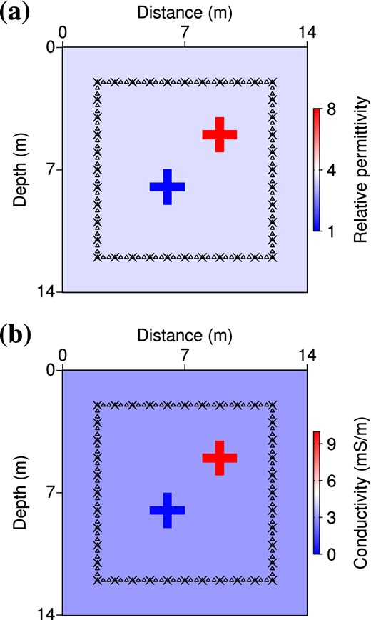
Acquisition setup and true models for permittivity (a) and conductivity (b), after Meles et al. (2011). Black crosses indicate source locations and receiver locations are marked with triangles. Note that we assume the antennas to be perpendicular to the plane of observation (TE mode), whereas Meles et al. (2011) use in-plane antennas (TM mode).

Figure 2.

Open in new tab Download slide

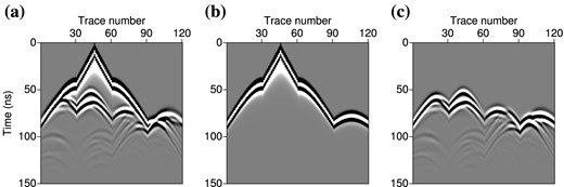
Time-domain shot gathers computed for the cross-shaped benchmark, (a) true model, (b) initial homogeneous model, (c) residuals. Data have been computed in the frequency-domain and convolved with the time-derivative of a Ricker wavelet of central frequency 100 MHz before inverse Fourier transform.

To perform the inversion, we first compute synthetic observed data in the true model of Fig. 1 for the seven following frequencies: 50, 60, 70, 80, 100, 150 and 200 MHz, which are consistent with the frequency bandwidth of a 100-MHz antenna. Note that we compute these observed data d_obs with the same modelling tool as the one used for computing the calculated data d_cal in the inversion process (inverse crime approach). The irregular frequency sampling is inspired by the strategy of Sirgue & Pratt (2004) who show that the wavenumber coverage increases with frequency (see their Fig. 3), so that a fine sampling of high frequencies is not required. We can perform inversion by considering the seven selected frequencies either simultaneously or through a sequential procedure where the initial model for each frequency is the final result of the previous inverted frequency. The sequential strategy based on the low to high-frequencies hierarchy has been promoted by Pratt & Worthington (1990) to mitigate non-linearities such as cycling skipping effects. On the other hand, the strategy of inverting simultaneously all frequencies is more subject to the cycle-skipping problem, depending on the initial model. But if a good initial model is available, it will take benefit from a broadband information. Finally, more elaborated strategies can be used. For instance, we may proceed through a cumulative sequential approach where we keep low-frequency data as we move to high frequencies as suggested by Bunks et al. (1995) for seismics in the time domain, and used by Meles et al. (2011) for GPR data inversion. In the frequency domain, it amounts to invert the following seven groups of cumulative frequencies:

Figure 3.

$Real part of the monochromatic electric fields diffracted by a permittivity anomaly (a) and a conductivity anomaly (b) at 100 MHz. Anomalies are located at the centre of the medium (x = 7 m, z = 7 m) and the black cross indicates the source location (x = 2 m, z = 7 m). Perturbation amplitudes are of 5 per cent of the homogeneous background values (δεr = 0.2 and δσ = 0.15 mS m−1).$

Open in new tab Download slide

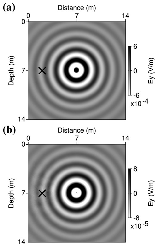
Real part of the monochromatic electric fields diffracted by a permittivity anomaly (a) and a conductivity anomaly (b) at 100 MHz. Anomalies are located at the centre of the medium (x = 7 m, z = 7 m) and the black cross indicates the source location (x = 2 m, z = 7 m). Perturbation amplitudes are of 5 per cent of the homogeneous background values (δε_r = 0.2 and δσ = 0.15 mS m⁻¹).

50

MHz,

50

60

MHz,

50

60

70

MHz,

⋅⋅⋅

50

60

70

80

100

150

200

MHz.

Open in new tab

Note that this approach, that we will call the Bunks’ strategy by analogy with the time domain, implies a consequent computational effort when applied in the frequency-domain. In the following, we will test the three above-mentioned strategies (simultaneous versus sequential versus Bunks’ strategy) and retain the most robust one for our realistic application.

3.1 Parameter sensitivity and trade-off

As we are interested in quantifying permittivity and conductivity values, we have to estimate the sensitivity of the data to these parameters. As done by Malinowski et al. (2011) for velocity and attenuation, we can evaluate the impact of both parameters in the data by computing the electric field that is diffracted by anomalies of permittivity and conductivity. Fig. 3 shows the real part of such monochromatic scattered fields u^sc(m, δm_i) at a frequency of 100 MHz, computed as the difference between the incident field u(m) emitted by a source in the homogeneous background |$\bf m$| of Fig. 1 and the field emitted by the same source in a perturbed medium m + δm_i where an anomaly δm_i of small amplitude has been added in the centre of the medium. We apply a perturbation amplitude of δp = 5 per cent of the background value, such that δm_i = δp × m_i, with i the index of the central cell in the finite-difference grid.

The scattered wavefield u^sc(m, δm_i) is linked to the partial derivative wavefield |$\partial _{m_i}{\bf u}$|⁠, which in turn can be related to the diffraction matrix by differentiating the forward problem (eq. 4) with respect to the model parameters, providing at first order

\begin{equation} {\bf u}^{sc}({\bf m},\delta m_i) \simeq \frac{\partial {\bf u}({\bf m})}{\partial m_i}\delta m_i = -\mathcal {A}^{-1}\frac{\partial \mathcal {A}}{\partial m_i}\,\delta m_i\,{\bf u}({\bf m}). \end{equation}

(10)

In eq. (10), the scattered wavefield can be interpreted as the field emitted by a virtual source |$\partial _{m_i}\mathcal {A}\,\delta m_i\,{\bf u}$| colocated with the anomaly δm_i and whose signature characterizes the data sensitivity to the considered parameter, contained in the diffraction matrix |$\partial _{m_i}\mathcal {A}$| (Pratt et al. 1998; Malinowski et al. 2011; Operto et al. 2013). This scattered field is the response of the anomaly to the incident field u(m) which controls its illumination, depending on the acquisition configuration and on the antenna radiation pattern. Therefore, the shape of the scattered wavefield entirely reflects the response of the anomaly and only depends on the sensitivity kernel |$\partial _{m_i}\mathcal {A}$|⁠, whereas its amplitude and phase partly come from the incident field, and thus from the GPR antenna.

As shown in Fig. 3, the fields diffracted by permittivity and conductivity anomalies in a homogeneous medium are both isotropic but have different amplitudes and phases. In Fig. 4, we present the amplitudes and phases of the diffracted fields as a function of the distance to the anomaly for different frequencies. Fig. 4(a) shows that the impact of the anomaly of permittivity is larger in amplitude than the one of conductivity in the frequency range we consider for GPR investigation (at least, for equal relative perturbations δp). In the general case, this amplitude ratio depends on the loss-tangent at grid point i, tan δ_i = σ_i/(ε_iω), that quantifies the energy dissipation in the dielectric lossy background, and on the relative perturbation amplitudes in permittivity δp^ε and conductivity δp^σ. Based on the expressions of the scattered wavefield (eq. 10) and of the diffraction matrices (eq. 9), we have

\begin{equation} \frac{{\bf u}^{sc}({\bf m},\delta \sigma _i)}{{\bf u}^{sc}({\bf m},\delta \varepsilon _i)} = \frac{\imath \omega \,\delta \sigma _i}{\omega ^2\,\delta \varepsilon _i} = \imath \frac{\sigma _i}{\varepsilon _i\omega }\frac{\delta p^\sigma }{\delta p^\varepsilon }. \end{equation}

(11)

In the frequency range of GPR investigations, EM waves encounter rather low-loss media, such that tan δ ≪ 1 (for instance, in the homogeneous background of Fig. 1, we have tan δ ≃ 0.14), so that data are intrinsically more sensitive to permittivity than to conductivity. However, it can be compensated by the fact that in natural media, conductivity may present more contrasts than permittivity (conductivity can vary over several order of magnitudes, typically from 10⁻⁴ to 0.1 S m⁻¹, whereas permittivity varies from 1 in air to 81 in water). Consequently, conductivity anomalies can have a significant imprint on the data. Moreover, eq. (11) and Fig. 4(a) show that, in a given medium, the sensitivity of the data to conductivity decreases with frequency relatively to the sensitivity to permittivity. Therefore, high-frequency information about low conductivity contrasts may be hidden below the noise level. Finally, another important feature in Fig. 4(b) is that diffractions of permittivity and conductivity present a 90° phase shift, as expected from the presence of the imaginary unit in eq. (11).

Figure 4.

$(a) Amplitudes of the diffracted fields for three frequencies. (b) Phases of the diffracted fields at 50 MHz.$

Open in new tab Download slide

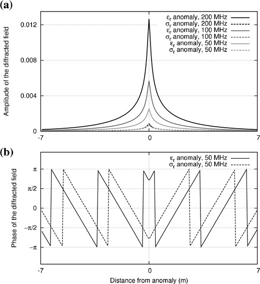
(a) Amplitudes of the diffracted fields for three frequencies. (b) Phases of the diffracted fields at 50 MHz.

From the differences in frequency-dependency and phase between the diffraction patterns of permittivity and conductivity, we can expect that both parameters could be reconstructed from recorded GPR data, provided that various angles of illumination and a wide frequency bandwidth are available to distinguish their respective signatures (Pratt et al. 1998; Operto et al. 2013). Conversely, a partial illumination and a reduced frequency bandwidth will induce a trade-off between both parameters, meaning that a wave scattered in one direction at one frequency by a permittivity anomaly can be equivalently explained by a conductivity anomaly shifted in space and of stronger amplitude.

To draw a parallel with the reconstruction of seismic velocity and attenuation, let us remark first that the imprint of conductivity in GPR data is generally stronger than the effect of the quality factor Q_P in seismic data (see the perturbations applied by Malinowski et al. 2011, and the resulting imprint relatively to velocity). In addition, the attenuation of electromagnetic waves do not suffer from the ambiguity discussed by Mulder & Hak (2009) and Hak & Mulder (2011): Even in low-loss media, the electromagnetic quality factor Q_EM ≃ 1/tan δ is frequency dependent. Seismic velocity and attenuation can only be distinguished by their phases, whereas the frequency dependency of the relative impact of permittivity and conductivity in the data is an additional information that may help to mitigate the trade-off between parameters.

We shall mention that the above discussion on the diffraction patterns of parameter anomalies is particularly adapted to on-ground GPR data, which mostly contain reflections and diffractions. Crosshole GPR data present other sensitivities to permittivity and conductivity. First because crosshole measurements are generally performed in TM mode, for which permittivity and conductivity act differently on the impedance matrix, so that their diffraction patterns are dipolar (independently from the dipolar radiation pattern of finite-line antennas in TM mode). To go further, it is not obvious that this kind of sensitivity analysis based on the diffraction patterns would be consistent when dealing with crosshole data, which mostly contain transmitted signal. In transmission regime, data might be more sensitive to extended anomalies which the waves pass through than to local diffracting points.

The previous remarks about the scattered wavefields have important consequences on the strategy required for multiparameter imaging. In a first approach, reasoning only on the loss tangent in eq. (11) tends to confirm the common mind that GPR data are mainly sensitive to permittivity, which justifies the use of alternated strategies: fixing the conductivity to an expected value and inverting for the permittivity in a first step, and then proceeding to the conductivity reconstruction with a fixed updated permittivity (Ernst et al. 2007). However, this strategy can fail to retrieve satisfactory models because, as shown in eq. (11), strong conductivity contrasts may have a significant imprint on the data (both on amplitudes and phases), which may hinder the reconstruction of an accurate permittivity model during the first step. In the second step, the conductivity reconstruction may then suffer from artifacts because it is very sensitive to the kinematic accuracy of the background medium (as is the reconstruction of attenuation in visco-acoustics, see e.g. Kamei & Pratt 2008, 2013). Because of the trade-offs, errors contained in the previously inverted permittivity, even if small, will systematically map into conductivity artifacts (for an interesting discussion on the effect of the trade-off, see Kamei & Pratt 2013 ; Section 3.3). As a consequence, simultaneous inversion of permittivity and conductivity generally yields better results than alternated or cascaded algorithms (Meles et al. 2010).

More elaborated schemes can consist in a first FWI step for the reconstruction of the permittivity while keeping fixed the conductivity, and in a second FWI step to invert simultaneously for permittivity and conductivity. It is a strategy used for the inversion of velocity v_P and attenuation Q_P in seismics (Kamei & Pratt 2008; Malinowski et al. 2011; Prieux et al. 2013; Kamei & Pratt 2013; Operto et al. 2013), where the parameter v_P is first reconstructed with an approximate estimation of a constant Q_P before the simultaneous inversion of the two parameters. This approach yields more satisfactory results because the first step improves the kinematic model for the second step, but a well-designed multiparameter scheme is still needed for the second step (if the initial model is accurate enough, we do not need the first step).

The design of multiparameter FWI is thus crucial but it faces a major problem when dealing with different parameter units and sensitivities (Meles et al. 2012). Meles et al. (2010) tackle this issue by introducing two descent step lengths in their algorithm: one for minimizing the misfit function in the gradient direction with respect to permittivity, and another in the direction of conductivity. This approach performs better than the one proposed by Ernst et al. (2007) because permittivity and conductivity models are updated simultaneously at each iteration (instead of every n iterations). But it amounts to consider the optimization with respect to permittivity and conductivity as two independent problems, and to neglect the possible trade-off between the two types of parameters. In this study, we propose to investigate a fully multiparameter strategy. The L-BFGS approximation of the inverse Hessian operator in the quasi-Newton scheme (7) should take the trade-offs between parameters into account.

3.2 Parameter scaling

To gather permittivity and conductivity in the model vector |$\bf m$|⁠, we have to consider adimensional quantities. It requires to define scales of measurement for the permittivity and the conductivity. The relative permittivity ε_r = ε/ε_o is commonly defined according to the vacuum permittivity ε_o ≃ 8.85 . 10⁻¹² F m⁻¹. In addition, we introduce a relative conductivity σ_r = σ/σ_o. By convention, we define the reference conductivity σ_o as the conductivity of a reference medium in which the loss tangent tan δ_o = σ_o/(ε_oω_o) equals one at a reference frequency f_o = 100 MHz. The reference frequency f_o = ω_o/(2π) corresponds to the central frequency of the band we will use in our numerical tests. We shall underline that this arbitrary definition is only a convention used for the optimization. In particular, the reference medium of permittivity ε_o and conductivity σ_o has nothing to do with the physical medium we want to investigate. This convention leads to the reference value σ_o = ε_oω_o ≃ 5.6 mS m⁻¹. The relative permittivity ε_r and the relative conductivity σ_r constitute the two classes of parameters we will use for the reconstruction.

Note that we could question the choice of ε_r and σ_r as the model parameters m_i to be optimized. Although we are interested in knowing the permittivity and the conductivity in the subsurface because they are meaningful physical quantities, other variables might be considered in the optimization procedure. We shall mention that we have investigated various couples of parameters (amoung others, |$\sqrt{\varepsilon _r}$|⁠, |$1/\sqrt{\varepsilon _r}$|⁠, ln (1 + σ_r), tan δ, …) and we did not found significant advantages for using these non-linear parameters compared to the choice of the relative permittivity ε_r and relative conductivity σ_r. On the contrary, inverting for the loss tangent tan δ = ε/(σω) should be avoided because it induces a strong coupling between permittivity and conductivity models. In addition, optimizing the parameters ε_r and σ_r enables to easily control the relative weight given to permittivity and conductivity in the inversion process, as we will discuss in the following. Thus, we consider linear combinations of the relative permittivity and of the relative conductivity of the form (ε_r, σ_r/β), where β is a dimensionless scaling factor which controls the weight of σ_r versus ε_r in the optimization process and may compensate for the arbitrary definition of the reference permittivity and reference conductivity. In the following, we refer to the reconstructed parameter σ_r/β as the scaled conductivity. We can now give explicit expressions for the model and gradient vectors:

\begin{equation} {\bf m}= {\left(\begin{array}{c}\bf \varepsilon _r \\ {\bf \sigma _r}/\beta \end{array}\right)}, \quad \mbox{and}\quad {\bf G}({\bf m}) = {\left(\begin{array}{c}\bf G^{\varepsilon _r}({\bf m}) \\ \beta {\bf G^{\sigma _r}({\bf m})} \end{array}\right)}. \end{equation}

(12)

Here, we shall remind that, although the gradient contains two distinct parts related to permittivity and conductivity, the descent direction is computed using the global gradient vector G(m_k) and the model update is performed using a unique step length α_k in eq. (7). The gradient components are deduced from eqs (8) and (9) using the chain rule such that

\begin{equation} \frac{\partial \mathcal {A}_{ij}}{\partial \varepsilon _{r_i}}=-\varepsilon _o\omega ^2\delta _{ij}, \quad \mbox{and}\quad \frac{\partial \mathcal {A}_{ij}}{\partial \sigma _{r_i}}=-\imath \sigma _o\omega \delta _{ij}. \end{equation}

(13)

Numerical experiments show that the inversion is very sensitive to the respective weights between the relative permittivity and the scaled conductivity in the optimization process, that is to the scales of measurement through the selected scaling factor β. On average, the relative weight of the scaled conductivity versus permittivity in the gradient is given by

\begin{equation} \frac{||\beta \bf G^{\sigma _r}||}{||\bf G^{\varepsilon _r}||} \simeq \beta \frac{||\partial _{\sigma _{r_j}}\mathcal {A}||}{||\partial _{\varepsilon _{r_j}}\mathcal {A}||} \propto \beta \frac{\sigma _o}{\varepsilon _o\omega }, \end{equation}

(14)

which is nothing other than the loss tangent tan δ_o(ω) of the reference medium with permittivity ε_o and conductivity σ_o at frequency ω, scaled by the factor β. According to our definition of the reference conductivity σ_o, the ratio of eq. (14) will then be about β for a group of frequencies centred around 100 MHz. Note that we recognize an expression for the gradient in eq. (12) that is similar to the preconditioned gradient proposed by Kamei & Pratt (2013). The difference in our case is that we consider the parameter σ_r/β, whose natural gradient is |$\beta {\bf G^{\sigma _r}}$|⁠. It is therefore a reparameterization, another way to scale the parameter space, and not a preconditioning. However, as in Kamei & Pratt (2013), the factor β will act as an implicit regularization: We will see that small values of β penalize the conductivity update (at the frequency 100 MHz, it corresponds to values of β < 1).

In eq. (7), the descent direction depends not only on the gradient, but also on the L-BFGS approximation of the Hessian |$\mathcal {B}$|⁠. Although this Hessian approximation is not readily available, understanding the structure of the Hessian through an approximate evaluation should shade light into the optimization procedure. The true Hessian |$\mathcal {H}$| of the misfit function reads

\begin{eqnarray} &&{\mathcal {H} = \mathcal {R}e{\left(\begin{array}{cc}\mathcal {J}^{\bf \varepsilon _r^{\dagger} }\mathcal {J}^{\bf \varepsilon _r} &\quad \beta \mathcal {J}^{\bf \varepsilon _r^{\dagger} }\mathcal {J}^{\bf \sigma _r} \\ \beta \mathcal {J}^{\bf \sigma _r^{\dagger} }\mathcal {J}^{\bf \varepsilon _r} &\quad \beta ^2\mathcal {J}^{\bf \sigma _r^{\dagger} }\mathcal {J}^{\bf \sigma _r} \end{array}\right)}} \nonumber\\ && + \,\mathcal {R}e\left\lbrace \sum _{i=1}^{N_D} \Delta d_i {\left(\begin{array}{cc}\displaystyle \frac{\partial ^2 d_{cal_i}}{\partial \varepsilon _{r_j} \partial \varepsilon _{r_l}} &\quad \beta \displaystyle \frac{\partial ^2 d_{cal_i}}{\partial \varepsilon _{r_j} \partial \sigma _{r_l}} \nonumber \\ \beta \displaystyle \frac{\partial ^2 d_{cal_i}}{\partial \sigma _{r_j} \partial \varepsilon _{r_l}} &\quad \beta ^2\displaystyle \frac{\partial ^2 d_{cal_i}}{\partial \sigma _{r_j} \partial \sigma _{r_l}} \end{array}\right)} _{ {{\begin{array}{c}j\in [\![1,N_M ]\!] \nonumber \\ l\in [\![1,N_M]\!] \end{array}}}} ^{\dagger} \right\rbrace .\nonumber \\ \end{eqnarray}

(15)

In this expression, for each data value i and each grid point j, the elements of the Jacobian matrices |$\mathcal {J}$| are defined by

\begin{equation} \mathcal {J}^{\varepsilon _r}_{ij} = \frac{\partial d_{cal_i}}{\partial \varepsilon _{r_j}} \quad \mbox{and}\quad \mathcal {J}^{\sigma _r}_{ij} = \frac{\partial d_{cal_i}}{\partial \sigma _{r_j}}. \end{equation}

(16)

In eq. (15), the first term corresponds to the linear part of the Hessian (Gauss-Newton). It accounts for geometrical spreading and dimensionalities of the parameters (diagonal terms), for the limited bandwidth effects due to the finite-frequency content of the source and to the partial illumination of the medium through the discrete acquisition setup (band-diagonal terms), and for the trade-offs between parameters (off-diagonal blocks). The second term accounts for double-scattered events with second-order derivatives of the wavefield which are neglected in Gauss-Newton approaches. The inverse Hessian approximated in eq. (7) should correct for all these effects and act as a deconvolution operator on the gradient (Pratt et al. 1998; Operto et al. 2013).

Figs 5(a)–(c) show three Hessian matrices |$\mathcal {H}^\beta$| for values of β ∈ {0.25, 1, 4}. These matrices have been computed using a finite-difference approximation around the final reconstructed models m^β = (ε_r, σ_r/β), which have been obtained inverting the seven frequencies between 50 and 200 MHz simultaneously, starting from the homogeneous background of Fig. 1. In these figures, we recognize the expected symmetric structure of the four blocks of the Hessian in eq. (15). Slight discrepancies in this symmetry are only due to numerical errors in the finite-difference approximation. The correlation between the parameters ε_r and σ_r/β represented in the off-diagonal blocks is not negligible, which justifies their consideration through efficient quasi-Newton methods for solving the multiparameter problem. The amplitude of the trade-off terms is particularly high in the corner of the subblocks (i.e. for cells located in the low-illuminated zone outside the acquisition system in Fig. 1). This is consistent with the result by Hak & Mulder (2010) that a partial illumination contributes to enhance the ambiguity between the different parameter types.

Figure 5.

$Hessians of the misfit function (a–c) and final models of conductivity (d–f) for three linear combinations of εr and σr/β, using a scaling factor β = 0.25 (a, d), β = 1 (b, e) and β = 4 (c, f). The final misfits C are expressed in fraction of the initial misfit Cinit.$

Open in new tab Download slide

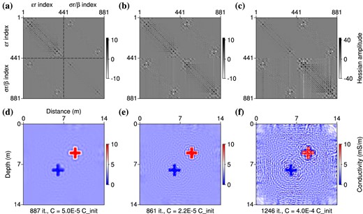
Hessians of the misfit function (a–c) and final models of conductivity (d–f) for three linear combinations of ε_r and σ_r/β, using a scaling factor β = 0.25 (a, d), β = 1 (b, e) and β = 4 (c, f). The final misfits C are expressed in fraction of the initial misfit C_init.

As expected from eq. (15), a scaling factor β = 1 provides four blocks of similar amplitudes (Fig. 5b). Alternatively, the value β = 0.25 penalizes the conductivity terms and gives more weight to the subblocks associated to permittivity (Fig. 5a), whereas the value β = 4 enhances the blocks related to conductivity (Fig. 5c). We present on Figs 5(d)–(f) the final conductivity models corresponding to the three values for the scaling factor β. The final images of conductivity are very sensitive to the parameter scaling through the selected factor β. Small values of β provide smooth reconstructions of conductivity (Fig. 5d), whereas large values of β enhance the contrasts, but also introduce instabilities (Figs 5e and f). Following Kamei & Pratt (2013), we can interpret the artifacts in the conductivity image as unphysical oscillations coming from the trade-off between permittivity and conductivity (monoparameter inversions of conductivity provide images without artifacts when the true permittivity model is known). In these tests, the reconstruction of the permittivity is less sensitive to the parameter scaling (all three values of β yield nearly identical, satisfactory results that we do not show). Further tests show that very large values of β > 10 provide smoother images of permittivity (and very high amplitude oscillations in conductivity), whereas very small values of β < 0.05 may also introduce instabilities in the image of permittivity, whereas the conductivity is not updated at all.

There are two possibilities to mitigate the undesired oscillations in the conductivity image. We can either penalize the relative conductivity with small values of the scaling factor β, as done by Kamei & Pratt (2013), or we can introduce a regularization term in the misfit function. Actually, both approaches are needed in the multiparameter permittivity-conductivity problem. The use of regularization may be the first choice in a common optimization procedure because the high amplitude oscillations in the conductivity model partly comes from the fact that the data are weakly sensitive to conductivity. To constrain the conductivity update, we introduce a Tikhonov regularization (Tikhonov & Arsenin 1977) through a model term C_M in the misfit function:

\begin{eqnarray} C({\bf m}) &=& C_D({\bf m})+\lambda C_M({\bf m}), \end{eqnarray}

(17)

with

\begin{eqnarray} C_M({\bf m}) &=& \frac{1}{2}{\bf \sigma _r}^T\mathcal {D}{\bf \sigma _r}. \end{eqnarray}

(18)

In this new misfit function, the first term C_D represents the fit to the data according to eq. (6). In the second term C_M, the matrix |$\mathcal {D}$| corresponds to the Laplacian operator, such that the minimization of the regularization term forces the conductivity model to be smooth. The hyperparameter λ is a weighting factor which balances the contribution of the regularization term with respect to the data term in the misfit function.

The gradient of the new misfit function (17) can also be expressed in terms of a data part and of a model part as

\begin{equation} {\bf G}({\bf m})= {\bf G}_D({\bf m})+\lambda {\bf G}_M({\bf m}), \end{equation}

(19)

where the data part G_D is computed after eqs (8) and (13) and the model part is

\begin{equation} {\bf G}_M={\left(\begin{array}{c}\bf 0 \\ \beta \mathcal {D}{\bf \sigma _r} \end{array}\right)}. \end{equation}

(20)

Note that we choose to regularize the relative conductivity σ_r and not the reconstructed parameter σ_r/β. Strictly speaking, both are equivalent because the scaling β would be absorbed in the regularization weight λ, but regularizing σ_r instead of σ_r/β is more convenient for further comparison of solutions obtained with a given regularization weight λ and different scaling factors β. In this synthetic case, we do not regularize the permittivity which is more constrained by the data. In real data cases, it may be necessary to constrain the permittivity update as well, using a smaller regularization weight than for conductivity.

Numerical tests involving regularization show that, in the case of β = 1, small values for the regularization weight λ slightly attenuate the very high-frequency artifacts in the image of Fig. 5(e). However, larger values of λ does not enable to remove entirely the remaining oscillations without degrading the shape of the reconstructed anomalies. In the case of β = 4, the Tikhonov regularization cannot both avoid the artifacts and provide a satisfactory reconstruction of the anomalies. The attenuation of the very high-amplitude oscillations requires a strong regularization which prevents the optimization from finding a satisfying minimization of the data misfit. Thus, regularization alone is not sufficient to design a stable inversion scheme. The parameter scaling through the scaling factor β is crucial both to avoid instabilities and obtain a satisfying resolution in the image of conductivity.

3.3 Behaviour of the inversion with respect to parameter scaling and frequency sampling

In this section, we try to understand in more details the effect of the scaling parameter β. Once we have selected the optimization technique, we expect that setting the scaling factor β will depend on the investigated medium, on the initial model, on the acquisition configuration, and on the frequency sampling strategy (because the relative impact of permittivity and conductivity in the data is frequency-dependent). In the following, we investigate the behaviour of the inversion process with respect to the scaling factor and to the frequency sampling strategy in the case of the cross-shaped benchmark with perfect illumination and without regularization. Although we proceed in the reconstruction of the parameters [ε_r, σ_r/β], we shall present results for the quantities [ε_r, σ] as they are those we understand physically.

First, we focus on the simultaneous frequency strategy, developing the case of Fig. 5. The Fig. 6 shows the evolution of the updated models of permittivity and conductivity, in the cases β = 1 (Fig. 6a) and β = 0.25 (Fig. 6b). We extract updated models at some iterations, corresponding to a given decrease of the misfit function C. In Fig. 6(a), we first note that instabilities in the conductivity image appear at early iterations (for C = 0.25 × C_init and C = 0.1 × C_init) and not at the end of the optimization. As a consequence, they are not due to the fact that the optimization fits numerical noise and cannot be avoided by stopping the iterative process earlier. It is also the reason why regularization fails to avoid instabilities when a non-adequate scaling factor is used. It is only when the permittivity is correctly reconstructed, providing a reliable kinematic background, that the image of conductivity converges towards the true one (C = 0.01 × C_init). Conversely, on Fig. 6(b) where more weight is given to permittivity, the permittivity model is reconstructed earlier in the iterations, whereas the reconstruction of conductivity is delayed and, thus, better retrieved when a more reliable kinematic model is available (C = 0.01 × C_init and C = 0.001 × C_init). This numerical test suggests that, even in the frame of a simultaneous reconstruction of permittivity and conductivity, the inversion should be led first by the permittivity update. However, there is a counterpart for this behaviour: As a strong penalization delays the reconstruction of conductivity, it induces a loss of resolution in the conductivity image for the same misfit decrease. An optimal value for the scaling factor β should both allow to avoid instabilities and to recover an image of conductivity that should be as complete and resolved as possible. The main limitation for achieving this goal is given by the maximal possible decrease of the misfit function (which depends mainly on the signal-over-noise ratio in the real data case).

Figure 6.

Open in new tab Download slide

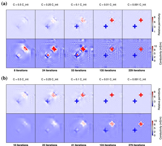
Evolution of permittivity and conductivity models along iterations using a scaling factor β = 1 (a) and β = 0.25 (b) when inverting for seven frequencies simultaneously.

Up to now, we have seen that the inversion path (Fig. 6), and even the final conductivity models (Fig. 5), strongly depend on the parameter scaling. This result is quite unexpected and suggests that the L-BFGS approximation of the Hessian correct only partially for parameter dimensionalities. We would like to better appreciate the exact performance of the L-BFGS algorithm. To illustrate the behaviour of the effective descent direction, we downgrade the example of Fig. 1 into an optimization in a two-parameter space. In this very simple problem, permittivity and conductivity in the background and in the blue cross are fixed at their true values and only the values in the red cross are allowed to vary. The anomaly is assumed to be homogeneous, such that the problem has only two degrees of freedom: ε_r and σ_r/β in the red cross. Fig. 7(a) presents a grid analysis of the misfit function for this two-parameter case. The misfit function has been evaluated for ε_r ranging in [1, 14] and σ ranging in [0, 27] mS m⁻¹, with the same acquisition setup as presented in Fig. 1 and for the seven frequencies simultaneously. We can notice on Fig. 7 that the misfit function is convex with a unique minimum. In addition, Fig. 7(a) shows the paths followed by the inversion for various values of the scaling factor β. All processes finally reach the global minimum but inversion paths are very sensitive to the parameter scaling as already observed in Fig. 6. Intuitively, large scaling factors β tends to orientate the inversion path along the conductivity axis.

Figure 7.

$Grid analysis of the misfit function on a simplified two-parameter problem. Dotted contours are spaced every 0.05 while dashed contours indicate particular levels of the misfit function (in fraction of the initial misfit). (a) Inversion paths in the physical domain (εr, σ) using various parameter scalings β. (b) Inversion path and gradients in the parameter domain (εr, σr/β) using a scaling factor β = 1.$

Open in new tab Download slide

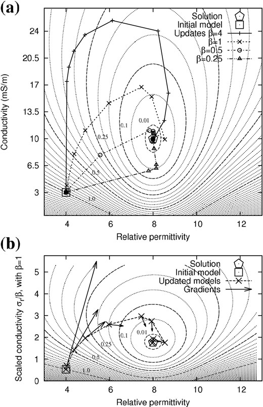
Grid analysis of the misfit function on a simplified two-parameter problem. Dotted contours are spaced every 0.05 while dashed contours indicate particular levels of the misfit function (in fraction of the initial misfit). (a) Inversion paths in the physical domain (ε_r, σ) using various parameter scalings β. (b) Inversion path and gradients in the parameter domain (ε_r, σ_r/β) using a scaling factor β = 1.

Fig. 7(b) shows the inversion path in the case of β = 1, mapped on a scaled view of the misfit function in the parameter space [ε_r, σ_r/β]. The arrows represent the opposite of the gradient vectors at each iteration: We can check that they are well orthogonal to the contours of the misfit function, indicating the steepest descent directions. Note that this case corresponds to a nearly circular misfit function in the vicinity of the solution, whereas larger scaling values would elongate the valley in the direction of permittivity, and thus would orientate the gradients in the direction of conductivity. This view of the misfit function in the parameter space, as seen by the optimization process, helps us to understand the behaviour of the L-BFGS algorithm. For iterations 1, 2 and 3, the descent directions computed by the L-BFGS-B technique (dashed lines between updated models) do not follow the steepest descent directions but are shifted towards the minimum. We can see here the benefit of the quasi-Newton approach which approximates the local curvature. But for later iterations (>4), the L-BFGS descent directions seem non-optimal compared to the steepest descent directions. This inertial effect is partly due to the old curvature information used by the L-BFGS algorithm to compute the local approximation of the Hessian.

Fig. 7 well illustrates that the parameter scaling deforms the parameter space and therefore modifies the descent directions computed by the L-BFGS-B algorithm. Although we could think about better approximations of the Hessian (e.g. preconditioned L-BFGS or truncated Newton methods, see Métivier et al. 2013, 2014), the optimization of permittivity and conductivity is likely to remain sensitive to the parameter scaling. As the problem is non-linear, the local descent directions on Fig. 7 cannot point directly to the global minimum of the misfit function, even with a good local estimation of the curvature (at least before being in the vicinity of the solution, where the quadratic approximation is more valid). In the two-parameter example, the inversion converges towards the unique minimum anyway because the problem is largely over-determined, but we speculate that the parameter scaling is of crucial importance for the high-dimensional case with the additional difficulty of secondary minima.

For this reason, the effect of non-linearity observed at early iterations in Fig. 6(a) is strongly dependent on the initial model we have selected, that is on how far the initial model is from the validity domain of the quadratic approximation. In particular, if we start from a good kinematic background, the updates of the conductivity model will be improved at early iterations. The initial model can be improved with the low-frequency content of the data if we adopt the low to high frequency hierarchy promoted by Pratt & Worthington (1990), inverting the seven frequencies sequentially.

Fig. 8 shows the permittivity and conductivity models obtained at the end of each mono-frequency step when inverting the seven frequencies sequentially, each model being the initial model for the next step. Again, we compare the use of a scaling factor equal to β = 1 (Fig. 8a) and β = 0.25 (Fig. 8b). As already observed when inverting the frequencies simultaneously, a low scaling factor β = 0.25 provides smoother results than the value β = 1, and the permittivity image is less sensitive to the parameter scaling. Despite the frequency hierarchy, the reconstruction of the conductivity model is not very satisfactory if a scaling factor β = 1 is used. In particular, the shape of the blue cross is degraded in Fig. 8(a), compared to the use of simultaneous frequencies (Fig. 5e). We may invoke two reasons to explain this. First, the consideration of simultaneous frequencies might help to better constrain the reconstruction of conductivity, as inferred from the frequency dependence of its diffraction pattern (Fig. 4). Secondly, in the sequential approach, the final reconstructed model results from the inversion of the highest frequency. Even if lower frequencies have been previously inverted, the final model thus contains a stronger finite-frequency imprint than using simultaneous frequencies.

Figure 8.

Open in new tab Download slide

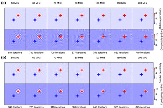
Evolution of the final reconstructed models for each step of the sequential inversion of the seven frequencies using scaling values β = 1 (a) and β = 0.25 (b).

The advantages of the frequency hierarchy and of a large frequency bandwidth can be combined using Bunks’ strategy. Further numerical tests involving Bunks’ strategy yields similar results as using the simultaneous strategy. Reconstructions are not significantly improved because this simple benchmark do not need a hierarchical approach. Since we choose a lower frequency bandwidth, we do not suffer from the cycle-skipping effect observed by Meles et al. (2011).

As a partial conclusion, we have shown on this perfect illumination case that an ad hoc scaling is needed between the relative permittivity and the relative conductivity in our quasi-Newton optimization scheme. This scaling should play a significant role for surface-to-surface acquisition because partial illumination tends to increase the ill-posedness of the inverse problem (Meles et al. 2012) as well as the trade-off between parameters (Hak & Mulder 2010).

Up to now, we have performed a quality control of the solution by comparison with the true model in an inverse crime way. In the following, we will propose a practical strategy for selecting a reasonable value for the scaling factor using an objective criterion.

4 A REALISTIC SYNTHETIC TEST

We now introduce a more realistic benchmark for the imaging of complex subsurface structures from multioffset on-ground GPR data. We first investigate the inversion of noise-free data with respect to the parameter scaling in order to establish a robust criterion for selecting the scaling factor β. In a second time, we add noise to the data to give an insight into the feasibility of the proposed workflow on real data.

4.1 Benchmark design

A realistic configuration has been designed for a 2-D distribution of permittivity (Fig. 9a) and conductivity (Fig. 9b) according to common-offset GPR profiles, a few common mid-point surveys, and electrical tomography measurements acquired at a test site located on recent fluvial deposits near Grenoble (France). We restrict the zone of interest to a 5-m-deep and 10-m-long section of the subsurface. The permittivity and conductivity values are in principle consistent with a silty soil (first layers) including lenses of clay (top right) above a 2- to 3-m-thick layer of relatively dry sands. The interface at around 3.8 m depth represents the water table. The 50-cm-thick zone above the zero z-level has values (ε_r = 1, σ = 0 S m⁻¹) of the air. This benchmark displays realistic but challenging sharp and large variations. In the subsurface, permittivity values range from 4 (main part in the middle) to 32 (layers of clay in the top right and at the bottom of the medium), and conductivity values range from 0.1 mS m⁻¹ (first layer) to 20 mS m⁻¹ (bottom layer). Maximal permittivity contrasts are of 1:10 at the air-ground interface, and of 4:22 in the subsurface (bottom of the main layer at z ≃ 3 m). Note the strongly attenuating layer at a depth of z = 3.5 m with a conductivity about σ = 10 mS m⁻¹, which may mask the underlying structures.

Figure 9.

Open in new tab Download slide

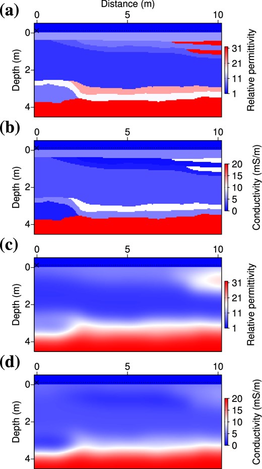
Realistic subsurface benchmark for permittivity (a, c) and conductivity (b, d). (a, b) True models. (c, d) Initial models. Sources and receivers are located 10 cm above the air-ground interface.

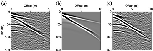
The medium is discretized on a 101 × 207 grid, with a grid step h = 5 cm. This meshing results in 20 907 grid points in the finite-difference modelling, and in 18 837 unknown values of permittivity and conductivity in the subsurface (values are kept fixed in the air, both to constrain the inversion and to avoid singularities at source and receiver locations). The acquisition setup consists in 41 source locations spaced every 0.25 m and in 101 receiver positions located every 0.1 m at a negative z-level of −0.1 m, that is two grid points above the air-ground interface. This setup is consistent with a multioffset experiment performed on the test site within a day. Initial models for permittivity (Fig. 9c) and conductivity (Fig. 9d) have been obtained by applying a gaussian smoothing to the true models with a correlation length τ = 50 cm. Only the main trends are depicted in the initial model and all details are erased, in particular the thin lenses in the top right of the medium but also the alternation of high and low values at depth (z ≃ 3.5 m). Fig. 10 shows the time-domain data computed in the true and initial models, for the first source of the acquisition array (at x = 0 m). In Fig. 10(a), three major reflections at t ≃ 20, 50, and 75 ns can be associated with the interfaces at z = 0.3, 2.5, and 3.8 m, while the diffractions at large offsets correspond to the thin lenses of clay. In Fig. 10(b), the initial model provides direct arrivals that are kinematically compatible with the observed data but the lack of contrasts does not reproduce the main reflected events and the diffractions are missing. Most of the data are not explained by the initial model and remain in the residuals (Fig. 10c).

Figure 10.

Open in new tab Download slide

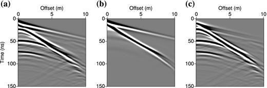
Time-domain shot gathers computed for the subsurface benchmark (Fig. 9) for the source located at x = 0 m, considering (a) the true model, (b) the initial model. (c) Initial residuals. Data have been computed in the frequency-domain and convolved with the time derivative of a Ricker wavelet of central frequency 100 MHz before inverse Fourier transform.

4.2 Inversion of noise-free data

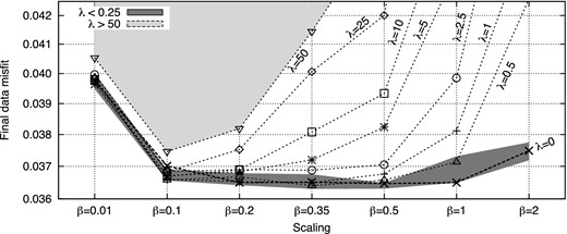
The frequency sampling is crucial for the imaging of such complex media. Therefore, we select a dense frequency sampling with 10 frequencies to be inverted: 50, 60, 70, 80, 90, 100, 125, 150, 175 and 200 MHz. Fig. 11 shows the final relative misfits obtained by inverting the ten frequencies simultaneously or adopting the so-called Bunks’ strategy which results here in ten groups of cumulative frequencies. These two strategies were quite equivalent in the cross-shaped benchmark with perfect illumination. For the imaging of more complex media with surface-to-surface illumination, Bunks’ strategy appears as the most efficient approach in terms of misfit decrease and provides more accurate models, because it presents the advantage both to proceed hierarchically and to end up with the inversion of the full frequency band. Again, the sequential strategy yields final reconstructed models that are less satisfactory, confirming the need for keeping the low frequency content in the hierarchical process. Therefore, we will use Bunks’ strategy in the following tests.

Figure 11.

Open in new tab Download slide

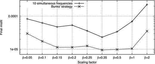
Final data misfit with respect to parameter scaling and frequency sampling strategy.

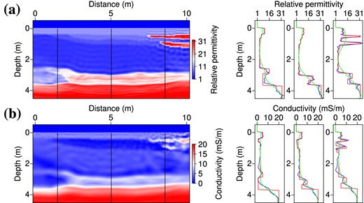
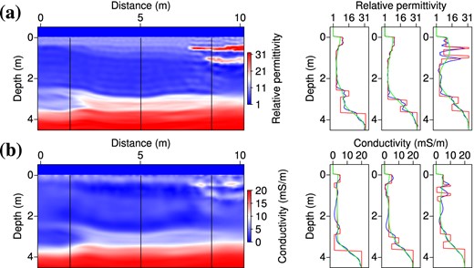
In Fig. 11, it must be noted that the misfit values reached using the Bunks’ strategy are quasi-independent from the parameter scaling in the range β ∈ [0.15, 1] (we do not apply any regularization here). However, the reconstructed models are very different and remain strongly sensitive to the scaling factor. Fig. 12 shows the permittivity and conductivity models obtained with scaling factor values of β = 0.15 and β = 1, which both have a misfit very close to 10⁻⁵ (in fraction of the initial misfit). As in the previous section, the value β = 0.15 provides a smooth conductivity model (Fig. 12c), whereas the value β = 1 (Fig. 12d) introduces instabilities and largely over-estimates the conductivity variations.

Figure 12.

Open in new tab Download slide

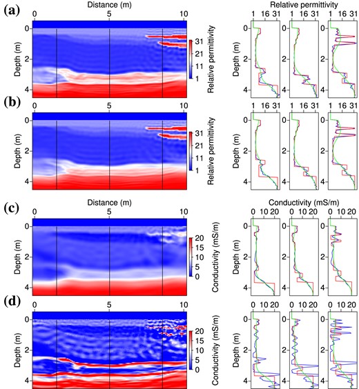
On the left: permittivity (a, b) and conductivity models (c, d) obtained by the inversion of noise-free data using scaling factors β = 0.15 (a, c) and β = 1 (b, d). On the right: vertical logs extracted along the black lines indicated on the 2-D sections. Red curves denote the true model, blue curves the inverted model and green curves the initial model. The optimization required about 350 iterations per frequency group (3448 and 3767 total iterations using β = 0.15 and β = 1, respectively).

The problem we face here is that we cannot discriminate between the two solutions of Fig. 12 with a criterion based only on the data misfit. This could suggest that the variations between the final models obtained with different β values of equivalent misfits all belong to the kernel (or null space) of the misfit function. Then we should conclude that we cannot recover a more precise information about the conductivity from the inverted data.

To have a more detailed insight into this problem, we can try to identify which spectral components differ between the solutions obtained using different scaling factors. To do so, we apply a k_z-transform to the conductivity logs of Figs 12(c) and (d). The corresponding amplitude spectra are shown in Fig. 13. On these spectra, we observe that the variations in the reconstruction are not restricted to the highest wavenumbers: Low wavenumbers are affected by the scaling as well. This result is quite unexpected because the small eigenvalues of the Hessian, related to the less constrained parameters, are generally related to small-scale structures (Hansen 2010, p.62). Our understanding is that discrepancies in the low wavenumbers should induce a degradation of the misfit but these discrepancies are compensated by high-wavenumber structures. If so, removing the high-wavenumber structures should cancel this compensation and lead to a degradation of the data misfit that would enable to distinguish the best models between the different solutions.

Figure 13.

Open in new tab Download slide

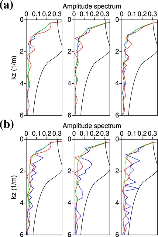
k_z-domain spectra of the vertical conductivity logs of Fig. 12 using a scaling factor β = 0.15 (a) and β = 1 (b). The black curves represent the low-pass filter applied both in x- and z-direction to the conductivity models in Fig. 14. Red curves denote the true model, blue curves the inverted model and green curves the initial model.

Fig. 14 shows low-pass filtered versions of the conductivity models of Fig. 12, where high wavenumbers k_x, k_z ≥ 2 are filtered out (both in the x- and z-directions). The threshold |$k_{x_{\rm max}}, k_{z_{\rm max}}=2$| roughly corresponds to the wavelengths propagating in the central part of the medium (where ε_r = 4) at 50 MHz, so it is rather a lower bound of the covered wavenumbers and it induces a quite drastic filtering. As expected from the differences in low-wavenumber contents in Fig. 13, the filtered models of Fig. 14 are still quite different but, since high wavenumbers have been filtered out, we can now discriminate between them: Computing the corresponding data misfit for these models, we find that the filtered conductivity model obtained with a scaling factor β = 0.15 (Fig. 14a) better explains the data than the one obtained with a value β = 1 (Fig. 14b) by a factor of ≃2.5.

Figure 14.

Open in new tab Download slide

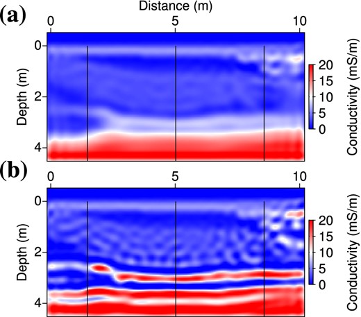
Filtered conductivity models corresponding to β = 0.15 (a) and β = 1 (b). Synthetic data computed in these filtered models yield data misfits C = 0.0017 × C_init and C = 0.0045 × C_init, respectively.

Consequently, we can expect that introducing a Tikhonov regularization in the misfit function will enable to identify conductivity solutions, by preventing the creation of the high-wavenumber structures that compensate for erroneous low-wavenumber reconstruction. As in the cross-shaped experiment, we regularize only the conductivity update following eqs (18) and (20). Fig. 15 shows the data misfit decrease obtained with the Bunks’ strategy when a Tikhonov regularization is introduced, as a function of the scaling factor β and for different regularization weights λ. As expected, the use of regularization makes the final data misfit more sensitive to the parameter scaling. Since it prevents the optimization to fit the data with high wavenumber structures, we can now discriminate between smooth reconstructed structures that well explain the data and those that do not. Varying the regularization weight λ, we can see on Fig. 15 that the more resolution we allow (with small λ values), the wider is the range of scaling factors β that well explain the data, and the more variability we get in the final conductivity models. Conversely, the more smoothness we impose (with large λ values), the less information we recover. For very large regularization weights λ > 1, we recover barely more than the initial model.

Figure 15.

Open in new tab Download slide

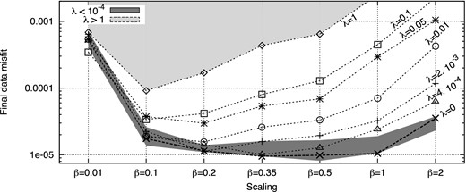
Final data misfit with respect to parameter scaling when a Tikhonov regularization is applied.

From Fig. 15, a reasonable criterion for selecting an adequate range of values for the scaling factor β and for the regularization weight λ is to seek for λ values that provide a satisfactory data fit on a small range of β values, that is regularization weights for which it exists a clear minimum of the data misfit with respect to the scaling factors. For instance, the regularization weight λ = 0.05 seems too large as it significantly degrades the data fit. Conversely, the weight λ = 4 . 10⁻⁴ is probably too small as it yields good data fits on a wide range of scaling values β ∈ [0.2, 0.5], which may provide dubious models. A reasonable range of values would therefore be λ ∈ [0.002, 0.01] for the regularization weight and β ∈ [0.1, 0.35] for the scaling factor.

Fig. 16 shows the model obtained with a scaling factor β = 0.2 and a regularization weight λ = 0.002. This solution is quite satisfactory when compared with the true model, suggesting that the proposed workflow for selecting the hyperparameters β and λ is pertinent. In particular, it shows that we can rely on the data misfit (without an arbitrary model criterion) for selecting a reasonable range for the parameter scaling β, in relation with an adequate regularization level λ for which it exists a clear minimum for the data misfit with respect to parameter scaling. We must underline the lower resolution of the conductivity reconstruction, resulting from the applied regularization (λ > 0) and penalization (β < 1). However, this solution provides a good compromise in the reconstruction of the high-permittivity, high-conductivity layer at z = 3 m, in spite of a slight shift in the conductivity image. The conductivity values in the thin lenses are comparable with those of the true model.

Figure 16.

Open in new tab Download slide

On the left: permittivity (a) and conductivity models (b) obtained by the inversion of noise-free data using a scaling factor β = 0.2 and a regularization weight λ = 0.002. On the right: vertical logs extracted along the black lines indicated on the 2-D sections. Red curves denote the true model, blue curves the inverted model and green curves the initial model. The optimization required about 330 iterations per frequency group (3379 total iterations).

As a partial conclusion, we have shown that the parameter scaling is even more crucial in this realistic case with surface-to-surface illumination than in the previous case with perfect illumination. Due to partial illumination, the inversion is less constrained and various scaling factors β can provide equivalent misfit decreases but very different solutions. Regularization is necessary to mitigate the ambiguity. By preventing the optimization to create high-wavenumber structures that artificially explain the data, regularization makes the final data misfit more sensitive to the scaling factor β. It is thus possible to determine a reasonable range of values both for the regularization weight λ and for the scaling factor β.

Fig. 17 summarizes the successive tests we performed in this section. Note that this diagram does not state for the final workflow that should be applied for multiparameter imaging, but rather as the reasoning flow that leads us to our multiparameter strategy. As indicated in the diagram, if performing regularized FWI still leads to different models of equivalent data misfits, then we can not discriminate between the different solutions based only on the data misfit, and we have to invoke a priori information to drive the inversion process towards a unique solution (see e.g. Asnaashari et al. 2013). Alternatively, we could have observed that only high wavenumbers differ between the models reconstructed with different scaling factors. Regularization would then have avoided the creation of the high-wavenumber artifacts and would probably have yielded similar solutions for the different scaling factors.

Figure 17.

Open in new tab Download slide

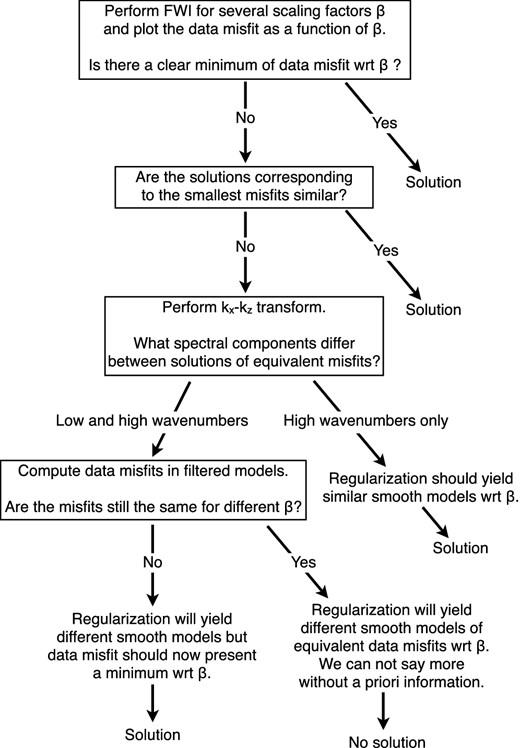
Flow diagram of the successive tests performed in Section 4 and of the related conclusions.

Finally, the retained workflow for multiparameter imaging would be:

Perform FWI with different parameter scalings β and regularization weights λ.
Plot the data misfit as a function of the scaling factor β, for each regularization weight λ.
Identify the regularization levels that exhibits a clear minimum of the data misfit with respect to parameter scaling. We shall choose the optimal (λ, β) combinations as the smallest λ values for which we can find such a minimum, and β values corresponding to this minimum.

We shall now see whether this workflow can be applied to noisy data, when noise may mask information about conductivity.

4.3 Inversion of noisy data

In order to tackle a more realistic example, white noise is added to the synthetic frequency data with a signal-over-noise ratio (SNR) of 25 dB. This noise level is consistent with the noise observed in real GPR data. Fig. 18 shows the impact of the noise on a time-domain shot gather. In the noisy data, the main reflected events are still visible but diffractions at large offsets are below the noise level.

Figure 18.

Open in new tab Download slide

Noisy time-domain shot gathers for the subsurface benchmark (source at x = 0 m). (a) Observed data, (b) data computed in the initial model. (c) Initial residuals. Data have been computed in the frequency-domain, then we applied a white noise of SNR = 25 dB in the frequency-domain before the convolution with the time-derivative of a Ricker wavelet of central frequency 100 MHz and inverse Fourier transform.

In Fig. 19, the thick dashed line shows the final data misfit decrease obtained with different values for the scaling factor, without regularization. The presence of noise in the data prevents to decrease the misfit function below a threshold of about 0.0365 (in fraction of the initial misfit). Again, we reach equivalent data misfits for very different scaling values β ∈ [0.2, 1]. Regularization is needed to constrain the conductivity model and discriminate between the different solutions. The other curves of Fig. 19 show the final data misfit reached using the same range of scaling factors β and various regularization weights λ. It presents the same features as in the case of noise-free data (Fig. 15), enabling to determine a range of reasonable values both for the scaling factor β and for the regularization weight λ on the single criterion of data misfit. Here, the smallest regularization weights that provide a satisfactory data fit on a small range of scaling factors β ∈ [0.1, 0.2] are λ = 5 to 10.

Figure 19.

Open in new tab Download slide

Final data misfit with respect to parameter scaling when a Tikhonov regularization is introduced in the inversion of noisy data (SNR = 25 dB).

Fig. 20 shows the inversion results obtained with a scaling factor β = 0.2 and a regularization weight λ = 5. In the permittivity image, thin superficial layers are still reconstructed quite accurately although the second lens is slightly shifted downwards. Resolution dramatically decreases with depth and the high-permittivity layer does not clearly appear. The strong regularization of conductivity only provides the main trend of the conductivity structures. The lenses of clay can be distinguished while a blurred image of the alternation of conductivity at depth is obtained. This result may seem disappointing but it should be underlined that the low resolution we obtain is the consequence of the applied regularization and penalization, which are necessary to not over-interprete the data.

Figure 20.

Open in new tab Download slide

On the left: permittivity (a) and conductivity models (b) obtained by the inversion of noisy data (SNR = 25 dB) using a scaling factor β = 0.2 and a regularization weight λ = 5. On the right: vertical logs extracted along the black lines indicated on the 2-D sections. Red curves denote the true model, blue curves the inverted model and green curves the initial model. The optimization required about 25 iterations per frequency group (241 total iterations).

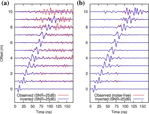
Finally, Fig. 21 compares the time-domain data computed in the inverted model of Fig. 20 with the observed noisy data (Fig. 21a) and with the observed noise-free data (Fig. 21b). For a better visualization of the signal at late arrival times and large offsets, we apply a time-varying gain and a trace-by-trace normalization (for each offset, the reference amplitude is the maximum of the observed trace). Every tenth trace is shown. It can be seen that noise is not fitted in the time-domain, although we did not regularize the permittivity update. It suggests that the L-BFGS optimization is robust with respect to noise, but it also may come from the fact that there does not exist any structure in the model space that could explain the applied noise, which is totally uncoherent. We expect to encounter more difficulties when dealing with coherent noise in real data (e.g. ringing effects). In Fig. 21(b), it appears that the added noise slightly damaged the fit in some parts of the radargram, especially in the zone related to the thin lenses (8 ≤ x ≤ 10 m). For comparison, it must be mentioned that synthetic data computed in the model of Fig. 16, which has been reconstructed by inverting noise-free data, perfectly match the observed data.

Figure 21.

Open in new tab Download slide

Time data fit. (a) Noisy observed data versus data calculated in the model of Fig. 20 obtained by inverting the noisy data. (b) Noise-free observed data versus the same data calculated in the inverted model of Fig. 20. A time-varying gain (×t) and trace-by-trace normalization have been applied.

5 DISCUSSION

We have shown that a robust reconstruction of permittivity and conductivity requires both parameter scaling and regularization. Here, we may comment the similarities and differences between these two ingredients, which may appear redundant but have actually distinct roles.

As shown in Fig. 5, small values for the scaling factor β penalize the conductivity updates and provide smooth conductivity models, as does regularization. Looking at the Hessian matrices, we can also note that penalizing the conductivity with a small scaling factor amounts to damp the small singular values of the Hessian, because the misfit function is more sensitive to permittivity than to conductivity. It is also the effect of Tikhonov regularization (Hansen 2010, p.62). Finally, parameter scaling and regularization both modify the shape of the global misfit function, and thus the inversion path, but in different ways we shall describe now.

Penalization of the conductivity update through the scaling factor β orientates the inversion path in the direction of permittivity, until a satisfying kinematic model is obtained (see Fig. 7). The conductivity model is then updated only on the basis of the data misfit decrease, without an explicit smoothness requirement. Potentially, an adequate parameter scaling can guide the inversion on a reasonable path towards the minimum of the data misfit C_D and this solution can present smooth parts as well as contrasts. Conversely, regularization attracts the inversion path towards a smooth conductivity model: The minimum of the global misfit function is then shifted towards the minimum of its model term C_M (in the two-parameter case of Fig. 7, it would be a valley located at σ = 3 mS m⁻¹). Consequently, the parameter scaling does not prevent the misfit function to converge, contrary to regularization which generally results in a lower convergence rate: The optimization stops when the updated models cannot both minimize the data misfit and satisfy the model smoothness requirement. As a conclusion, the role of the parameter scaling is to guide the inversion on a reasonable path, according to the sensitivity of the data, whereas regularization constrains the conductivity update, prevents the creation of high-wavenumber structures, and thus enables us to discriminate between low-wavenumber reconstructions that well explain the data or not (Fig. 15). Indeed, the inversion results using small values for the scaling factors (e.g. β = 0.2) are very similar with and without regularization (e.g. λ = 5 versus λ = 0 in the noisy data case) because the penalization of conductivity through the scaling factor already acts as a regularization. The principal role of regularization in our workflow is to tell us which smooth solution is convenient regarding the fit to the data.

6 CONCLUSION

In this study, we have presented a FWI algorithm of on-ground GPR data for the simultaneous reconstruction of permittivity and conductivity in 2-D. The inverse problem has been formulated in the frequency-domain as the minimization of the misfit to the data in a least-square sense. A model term is added to constrain the inversion with a Tikhonov regularization. The gradient of the misfit function is defined in the whole parameter space and is computed with the adjoint state method. The optimization is performed with a quasi-Newton scheme using the L-BFGS-B algorithm to economically estimate the effect of the Hessian on the parameter update.

Tests performed on a synthetic benchmark from the literature shows that the respective weights of permittivity and conductivity in the optimization process is of prior importance. A parameter scaling is introduced through a penalization of the conductivity parameter. Without an adequate value for this scaling factor, regularization alone cannot provide satisfactory results. The adequate value for the parameter scaling mainly depends on the respective sensitivity of the data to permittivity and conductivity, and to the quality of the initial model. With a weak sensitivity to conductivity and a poor initial model, more weight must be given to the permittivity parameter to give priority to the kinematic reconstruction before reconstructing the conductivity. The sensitivity of the reconstructions to the parameter scaling suggests that the L-BFGS algorithm does not correctly scale the descent direction with respect to different parameter types. We underline the need for investigating more complete approximations of the Hessian (e.g. truncated Newton methods, Métivier et al. 2013) to understand if more information can be extracted from the curvature of the misfit function.

The behaviour of the inversion with respect to frequency sampling has been investigating. As the relative impact of permittivity and conductivity varies with frequency, the reconstruction of both parameters takes a significant benefit from the simultaneous inversion of data with a broad frequency bandwidth. Therefore, simultaneous or cumulative frequency sampling strategies should be favoured, depending on the quality of the initial model.

The algorithm has also been tested on a more realistic benchmark, with a multi-offset, surface-to-surface acquisition configuration. In this case, various parameter scalings can lead to the same misfit decrease but to very different solutions. Regularization is needed to constrain the conductivity update and reduce the ambiguity. In the synthetic case we investigate, it is possible to find a range of reasonable values for both the scaling factor and the regularization weight, based only on the data misfit analysis. This workflow can be applied to extract a reliable information about conductivity from noisy data. We shall mention that, in some cases, it could be impossible to constrain the solution based only on the data misfit, and we underline the interest of introducing a priori information in the FWI process (Asnaashari et al. 2013).

The proposed workflow implying parameter scaling and regularization enables us to consider the inversion of real data in the near future. Common obstacles to real data inversion are 3-D to 2-D conversion, the design of a compatible initial model, and the estimation of the source signal, which must be integrated in the iterative process. Since first traveltime and amplitude tomography can not be performed from on-ground GPR data (contrary to crosshole data), the design of initial models for permittivity and conductivity from on-ground GPR data will be particularly challenging.

We would like to thank the SEISCOPE consortium for significant contribution (http://seiscope2.osug.fr). This work was performed by accessing to the high-performance computing facilities of CIMENT (Université de Grenoble) and of GENCI-CINES under grant 046091. We gratefully acknowledge both of these facilities and the support of their staff. We also thank an anonymous reviewer for its recommendations that helped to improve the clarity of the manuscript.

REFERENCES

Asnaashari

A.

,

Brossier

R.

,

Garambois

S.

,

Audebert

F.

,

Thore

P.

,

Virieux

J.

.

Regularized seismic full waveform inversion with prior model information

,

Geophysics

,

2013

, vol.

78

2

(pg.

R25

-

R36

)

Berenger

J.-P.

.

A perfectly matched layer for absorption of electromagnetic waves

,

J. Comput. Phys.

,

1994

, vol.

114

(pg.

185

-

200

)

Bradford

J.H.

.

Measuring water content heterogeneity using multifold GPR with reflection tomography

,

Vadose Zone J.

,

2008

, vol.

7

1

(pg.

184

-

193

)

Bunks

C.

,

Salek

F.M.

,

Zaleski

S.

,

Chavent

G.

.

Multiscale seismic waveform inversion

,

Geophysics

,

1995

, vol.

60

5

(pg.

1457

-

1473

)

Busch

S.

,

van der Kruk

J.

,

Bikowski

J.

,

Vereecken

H.

.

Quantitative conductivity and permittivity estimation using full-waveform inversion of on-ground GPR data

,

Geophysics

,

2012

, vol.

77

6

(pg.

H79

-

H91

)

Byrd

R.

,

Lu

P.

,

Nocedal

J.

.

A limited memory algorithm for bound constrained optimization

,

SIAM J. Sci. Stat. Comput.

,

1995

, vol.

16

(pg.

1190

-

1208

)

Cai

W.

,

Qin

F.

,

Schuster

G.T.

.

Electromagnetic velocity inversion using 2-D Maxwell's equations

,

Geophysics

,

1996

, vol.

61

4

(pg.

1007

-

1021

)

Carcione

J.M.

,

Cavallini

F.

.

On the acoustic-electromagnetic analogy

,

Wave Motion

,

1995

, vol.

21

(pg.

149

-

162

)

Cordua

K.S.

,

Hansen

T.M.

,

Mosegaard

K.

.

Monte Carlo full-waveform inversion of crosshole GPR data using multiple-point geostatistical a priori information

,

Geophysics

,

2012

, vol.

77

2

(pg.

H19

-

H31

)

Day-Lewis

F.D.

,

Singha

K.

,

Binley

A.M.

.

Applying petrophysical models to radar travel time and electrical resistivity tomograms: resolution-dependent limitations

,

J. geophys. Res.

,

2005

, vol.

110

doi:10.1029/2004JB003569

Google Scholar

OpenURL Placeholder Text

WorldCat

Deeds

J.

,

Bradford

J.

.

Characterization of an aquitard and direct detection of LNAPL at Hill Air Force base using GPR AVO and migration velocity analyses

,

Proceedings of 9th International Conference on Ground Penetrating Radar

,

2002

SPIE proceedings series

(pg.

323

-

329

)

Vol 4758

Google Scholar

OpenURL Placeholder Text

WorldCat

Deparis

J.

,

Garambois

S.

.

On the use of dispersive APVO GPR curves for thin-bed properties estimation: theory and application to fracture characterization

,

Geophysics

,

2009

, vol.

74

1

(pg.

J1

-

J12

)

El Bouajaji

M.

,

Lanteri

S.

,

Yedlin

M.

.

Discontinuous galerkin frequency domain forward modelling for the inversion of electric permittivity in the 2D case

,

Geophys. Prospect.

,

2011

, vol.

59

5

(pg.

920

-

933

)

Google Scholar

OpenURL Placeholder Text

WorldCat

Ellefsen

K.J.

,

Mazzella

A.T.

,

Horton

R.J.

,

McKenna

J.R.

.

Phase and amplitude inversion of crosswell radar data

,

Geophysics

,

2011

, vol.

76

3

(pg.

J1

-

J12

)

Ernst

J.R.

,

Green

A.G.

,

Maurer

H.

,

Holliger

K.

.

Application of a new 2D time-domain full-waveform inversion scheme to crosshole radar data

,

Geophysics

,

2007

, vol.

72

5

(pg.

J53

-

J64

)

Fischer

E.

,

McMechan

G.A.

,

Annan

A.P.

.

Acquisition and processing of wide-aperture ground-penetrating radar data

,

Geophysics

,

1992a

, vol.

57

3

(pg.

495

-

504

)

Fischer

E.

,

McMechan

G.A.

,

Annan

A.P.

,

Cosway

S.W.

.

Examples of reverse-time migration of single-channel, ground-penetrating radar profiles

,

Geophysics

,

1992b

, vol.

57

4

(pg.

577

-

586

)

Garambois

S.

,

Sénéchal

P.

,

Perroud

H.

.

On the use of combined geophysical methods to assess water content and water conductivity of near-surface formations

,

J. Hydrol.

,

2002

, vol.

259

(pg.

32

-

48

)

Gerhards

H.

,

Wollschläger

U.

,

Yu

Q.

,

Schiwek

P.

,

Pan

X.

,

Roth

K.

.

Continuous and simultaneous measurement of reflector depth and average soil-water content with multichannel ground-penetrating radar

,

Geophysics

,

2008

, vol.

73

4

(pg.

J15

-

J23

)

Gloaguen

E.

,

Marcotte

D.

,

Chouteau

M.

,

Perroud

H.

.

Borehole radar velocity inversion using cokriging and cosimulation

,

J. appl. Geophys.

,

2005

, vol.

57

(pg.

242

-

259

)

Grasmueck

M.

,

Weger

R.

,

Horstmeyer

H.

.

Full-resolution 3D GPR imaging

,

Geophysics

,

2005

, vol.

70

1

(pg.

K12

-

K19

)

Greaves

R.J.

,

Lesmes

D.P.

,

Lee

J.M.

,

Toksöz

M.N.

.

Velocity variations and water content estimated from multi-offset, ground-penetrating radar

,

Geophysics

,

1996

, vol.

61

3

(pg.

683

-

695

)

Hak

B.

,

Mulder

W.A.

.

Migration for velocity and attenuation perturbations

,

Geophys. Prospect.

,

2010

, vol.

58

(pg.

939

-

951

)

Google Scholar

OpenURL Placeholder Text

WorldCat

Hak

B.

,

Mulder

W.A.

.

Seismic attenuation imaging with causality

,

Geophys. J. Int.

,

2011

, vol.

184

1

(pg.

439

-

451

)

Hansen

P.C.

. ,

Discrete Inverse Problems: Insight and Algorithms

,

2010

SIAM

Google Scholar

Google Preview

OpenURL Placeholder Text

WorldCat

Hollender

F.

,

Tillard

S.

.

Modeling ground-penetrating radar wave propagation and reflection with the Jonscher parameterization

,

Geophysics

,

1998

, vol.

63

6

(pg.

1933

-

1942

)

Holliger

K.

,

Musil

M.

,

Maurer

H.

.

Ray-based amplitude tomography for crosshole georadar data: a numerical assessment

,

J. appl. Geophys.

,

2001

, vol.

47

(pg.

285

-

298

)

Huisman

J.A.

,

Hubbard

S.S.

,

Redman

J.D.

,

Annan

A.P.

.

Measuring soil water content with ground penetrating radar: a review

,

Vadose Zone J.

,

2003

, vol.

2

(pg.

476

-

491

)

Hustedt

B.

,

Operto

S.

,

Virieux

J.

.

Mixed-grid and staggered-grid finite difference methods for frequency domain acoustic wave modelling

,

Geophys. J. Int.

,

2004

, vol.

157

(pg.

1269

-

1296

)

Ihamouten

A.

,

Villain

G.

,

Dérobert

X.

.

Complex permittivity frequency variations from multioffset GPR data: hydraulic concrete characterization

,

IEEE Trans. Geosci. Remote Sens.

,

2012

, vol.

61

6

(pg.

1636

-

1648

)

Google Scholar

OpenURL Placeholder Text

WorldCat

Kalogeropoulos

A.

,

van der Kruk

J.

,

Hugenschmidt

J.

,

Busch

S.

,

Merz

K.

.

Chlorides and moisture assessment in concrete by GPR full waveform inversion

,

Near Surface Geophys.

,

2011

, vol.

9

3

(pg.

277

-

285

)

Kalogeropoulos

A.

,

van der Kruk

J.

,

Hugenschmidt

J.

,

Bikowski

J.

,

Brühwiler

E.

.

Full-waveform GPR inversion to assess chloride gradients in concrete

,

NDT&E Int.

,

2013

, vol.

57

(pg.

74

-

84

)

Kamei

R.

,

Pratt

R.G.

.

Waveform tomography strategies for imaging attenuation structure for cross-hole data

,

Extended Abstracts

,

2008

pg.

F019

Google Scholar

OpenURL Placeholder Text

WorldCat

Kamei

R.

,

Pratt

R.G.

.

Inversion strategies for visco-acoustic waveform inversion

,

Geophys. J. Int.

,

2013

, vol.

194

(pg.

859

-

894

)

Klotzsche

A.

,

van der Kruk

J.

,

Meles

G.A.

,

Doetsch

J.A.

,

Maurer

H.

,

Linde

N.

.

Full-waveform inversion of cross-hole ground-penetrating radar data to characterize a gravel aquifer close to the Thur River, Switzerland

,

Near Surface Geophys.

,

2010

, vol.

8

(pg.

635

-

649

)

Klotzsche

A.

,

van der Kruk

J.

,

Meles

G.A.

,

Vereecken

H.

.

Crosshole GPR full-waveform inversion of waveguides acting as preferential flow paths within aquifer systems

,

Geophysics

,

2012

, vol.

77

4

(pg.

H57

-

H62

)

Lailly

P.

.

The seismic inverse problem as a sequence of before-stack migrations

,

Conference on Inverse Scattering: Theory and Applications

,

1983

SIAM

(pg.

206

-

220

)

Google Scholar

OpenURL Placeholder Text

WorldCat

Lambot

S.

,

Weihermüller

L.

,

Huisman

J.A.

,

Vereecken

H.

,

Vanclooster

M.

,

Slob

E.C.

.

Analysis of air-launched ground-penetrating radar techniques to measure the soil surface water content

,

Water Resour. Res.

,

2006

, vol.

42

pg.

W11403

doi:10.1029/2006WR005097

Lopes

F.

.

Inversion des formes d'ondes électromagnétiques de données radar (GPR) multioffsets

,

PhD thesis

,

2009

Université Denis Diderot Paris 7

Google Scholar

OpenURL Placeholder Text

WorldCat

Malinowski

M.

,

Operto

S.

,

Ribodetti

A.

.

High-resolution seismic attenuation imaging from wide-aperture onshore data by visco-acoustic frequency-domain full waveform inversion

,

Geophys. J. Int.

,

2011

, vol.

186

3

(pg.

1179

-

1204

)

Meles

G.A.

,

van der Kruk

J.

,

Greenhalgh

S.A.

,

Ernst

J.R.

,

Maurer

H.

,

Green

A.G.

.

A new vector waveform inversion algorithm for simultaneous updating of conductivity and permittivity parameters from combination crosshole/borehole-to-surface GPR data

,

IEEE Trans. Geosci. Remote Sens.

,

2010

, vol.

48

(pg.

3391

-

3407

)

Meles

G.A.

,

Greenhalgh

S.

,

van der Kruk

J.

,

Green

A.G.

,

Maurer

H.

.

Taming the non-linearity problem in GPR full-waveform inversion for high contrast media

,

J. appl. Geophys.

,

2011

, vol.

73

(pg.

174

-

186

)

Meles

G.A.

,

Greenhalgh

S.A.

,

Green

A.G.

,

Maurer

H.

,

van der Kruk

J.

.

GPR full-waveform sensitivity and resolution analysis using an FDTD adjoint method

,

IEEE Trans. Geosci. Remote Sens.

,

2012

, vol.

50

5

(pg.

1881

-

1896

)

Métivier

L.

,

Brossier

R.

,

Virieux

J.

,

Operto

S.

.

Full waveform inversion and the truncated newton method

,

SIAM J. Sci. Comput.

,

2013

, vol.

35

2

(pg.

B401

-

B437

)

Métivier

L.

,

Bretaudeau

F.

,

Brossier

R.

,

Operto

S.

,

Virieux

J.

.

Full waveform inversion and the truncated newton method: quantitative imaging of complex subsurface structures

,

Geophys. Prospect.

,

2014

in press

Google Scholar

OpenURL Placeholder Text

WorldCat

Minet

J.

,

Lambot

S.

,

Slob

E.C.

,

Vanclooster

M.

.

Soil surface water content estimation by full-waveform GPR signal inversion in the presence of thin layers

,

IEEE Trans. Geosci. Remote Sens.

,

2010

, vol.

48

3

(pg.

1138

-

1150

)

Mulder

W.A.

,

Hak

B.

.

An ambiguity in attenuation scattering imaging

,

Geophys. J. Int.

,

2009

, vol.

178

(pg.

1614

-

1624

)

MUMPS-team

MUMPS—MUltifrontal Massively Parallel Solver users’ guide—version 4.9.2, ENSEEIHT-ENS Lyon

,

2009

Available at: http://www.enseeiht.fr/apo/MUMPS/ or http://graal.ens-lyon.fr/MUMPS(accessed 30 November 2013)

OpenURL Placeholder Text

WorldCat

Musil

M.

,

Maurer

H.

,

Holliger

K.

,

Green

A.G.

.

Internal structure of an alpine rock glacier based on crosshole georadar traveltimes and amplitudes

,

Geophys. Prospect.

,

2006

, vol.

54

(pg.

273

-

285

)

Nocedal

J.

,

Wright

S.J.

. ,

Numerical Optimization

,

2006

2nd edn

Springer

Operto

S.

,

Brossier

R.

,

Gholami

Y.

,

Métivier

L.

,

Prieux

V.

,

Ribodetti

A.

,

Virieux

J.

.

A guided tour of multiparameter full waveform inversion for multicomponent data: from theory to practice

,

Leading Edge

,

2013

September, Special section: Full Waveform Inversion

(pg.

1040

-

1054

)

Google Scholar

OpenURL Placeholder Text

WorldCat

Patriarca

C.

,

Lambot

S.

,

Mahmoudzadeh

M.R.

,

Minet

J.

,

Slob

E.

.

Reconstruction of sub-wavelength fractures and physical properties of masonry media using full-waveform inversion of proximal penetrating radar

,

J. appl. Geophys.

,

2011

, vol.

74

(pg.

26

-

37

)

Plessix

R.E.

.

A review of the adjoint-state method for computing the gradient of a functional with geophysical applications

,

Geophys. J. Int.

,

2006

, vol.

167

2

(pg.

495

-

503

)

Pratt

R.G.

,

Worthington

M.H.

.

Inverse theory applied to multi-source cross-hole tomography. Part I: acoustic wave-equation method

,

Geophys. Prospect.

,

1990

, vol.

38

(pg.

287

-

310

)

Pratt

R.G.

,

Shin

C.

,

Hicks

G.J.

.

Gauss-Newton and full Newton methods in frequency-space seismic waveform inversion

,

Geophys. J. Int.

,

1998

, vol.

133

(pg.

341

-

362

)

Prieux

V.

,

Brossier

R.

,

Operto

S.

,

Virieux

J.

.

Multiparameter full waveform inversion of multicomponent OBC data from valhall. Part 1: imaging compressional wavespeed, density and attenuation

,

Geophys. J. Int.

,

2013

, vol.

194

3

(pg.

1640

-

1664

)

Sirgue

L.

,

Pratt

R.G.

.

Efficient waveform inversion and imaging: a strategy for selecting temporal frequencies

,

Geophysics

,

2004

, vol.

69

1

(pg.

231

-

248

)

Tarantola

A.

.

Inversion of seismic reflection data in the acoustic approximation

,

Geophysics

,

1984

, vol.

49

8

(pg.

1259

-

1266

)

Tikhonov

A.

,

Arsenin

V.

. ,

Solution of Ill-Posed Problems

,

1977

Winston

Virieux

J.

,

Operto

S.

.

An overview of full waveform inversion in exploration geophysics

,

Geophysics

,

2009

, vol.

74

6

(pg.

WCC1

-

WCC26

)

Weihermüller

L.

,

Huisman

J.A.

,

Lambot

S.

,

Herbst

M.

,

Vereecken

H.

.

Mapping the spatial variation of soil water content at the field scale with different ground penetrating radar techniques

,

J. Hydrol.

,

2007

, vol.

340

(pg.

205

-

216

)

Yang

X.

,

van der Kruk

J.

,

Bikowski

J.

,

Kumbhar

P.

,

Vereecken

H.

,

Meles

G.

.

Full-waveform inversion of GPR data in frequency-domain

,

Proceedings of 14th International Conference on Ground Penetrating Radar

,

2012

(pg.

324

-

328

)

Google Scholar

OpenURL Placeholder Text

WorldCat

Download all slides

Month:	Total Views:
December 2016	2
February 2017	17
March 2017	15
April 2017	14
May 2017	6
June 2017	6
July 2017	12
August 2017	8
September 2017	6
October 2017	13
November 2017	2
December 2017	27
January 2018	22
February 2018	17
March 2018	43
April 2018	21
May 2018	20
June 2018	25
July 2018	21
August 2018	11
September 2018	23
October 2018	32
November 2018	14
December 2018	29
January 2019	29
February 2019	24
March 2019	46
April 2019	24
May 2019	17
June 2019	19
July 2019	31
August 2019	46
September 2019	15
October 2019	26
November 2019	17
December 2019	22
January 2020	20
February 2020	19
March 2020	25
April 2020	17
May 2020	17
June 2020	13
July 2020	39
August 2020	22
September 2020	25
October 2020	26
November 2020	29
December 2020	31
January 2021	27
February 2021	22
March 2021	25
April 2021	26
May 2021	34
June 2021	12
July 2021	18
August 2021	17
September 2021	40
October 2021	22
November 2021	38
December 2021	35
January 2022	13
February 2022	21
March 2022	28
April 2022	54
May 2022	21
June 2022	29
July 2022	21
August 2022	27
September 2022	27
October 2022	63
November 2022	34
December 2022	28
January 2023	14
February 2023	15
March 2023	22
April 2023	32
May 2023	40
June 2023	20
July 2023	43
August 2023	31
September 2023	29
October 2023	29
November 2023	20
December 2023	24
January 2024	21
February 2024	30
March 2024	61
April 2024	11

Article Contents

Two-dimensional permittivity and conductivity imaging by full waveform inversion of multioffset GPR data: a frequency-domain quasi-Newton approach

Abstract

1 INTRODUCTION

2 FORWARD AND INVERSE PROBLEMS FORMULATION IN THE FREQUENCY DOMAIN

2.1 Forward problem

2.2 Inverse problem

3 MULTIPARAMETER IMAGING OF PERMITTIVITY AND CONDUCTIVITY

3.1 Parameter sensitivity and trade-off

3.2 Parameter scaling

3.3 Behaviour of the inversion with respect to parameter scaling and frequency sampling

4 A REALISTIC SYNTHETIC TEST

4.1 Benchmark design

4.2 Inversion of noise-free data

4.3 Inversion of noisy data

5 DISCUSSION

6 CONCLUSION

REFERENCES

Citations

Views

Altmetric

Email alerts

Astrophysics Data System

Citing articles via

Latest

Most Read

Most Cited

Article Contents

Two-dimensional permittivity and conductivity imaging by full waveform inversion of multioffset GPR data: a frequency-domain quasi-Newton approach

Abstract

1 INTRODUCTION

2 FORWARD AND INVERSE PROBLEMS FORMULATION IN THE FREQUENCY DOMAIN

2.1 Forward problem

2.2 Inverse problem

3 MULTIPARAMETER IMAGING OF PERMITTIVITY AND CONDUCTIVITY

3.1 Parameter sensitivity and trade-off

3.2 Parameter scaling

3.3 Behaviour of the inversion with respect to parameter scaling and frequency sampling

4 A REALISTIC SYNTHETIC TEST

4.1 Benchmark design

4.2 Inversion of noise-free data

4.3 Inversion of noisy data

5 DISCUSSION

6 CONCLUSION

REFERENCES

Citations

Views

Altmetric

Email alerts

Astrophysics Data System

Citing articles via

Latest

Most Read

Most Cited

This Feature Is Available To Subscribers Only