1. Introduction
In the analysis of time series, change points are typically defined as those time points where we observe sudden changes in the data. These changes are often produced by events that can be internal or external to the nature of the process, and therefore, in order to properly understand the impact and nature of such events, it is important to accurately identify the time points where changes occur in the time series of interest. For this reason, change point detection (CPD) methods have been applied in different fields, including speech recognition [
1], climate change [
2], medicine [
3] and finance [
4], to name a few.
Multiple algorithms have been proposed to identify change points, including binary segmentation, mixture models and some Bayesian methods; see [
5]. In this work, we apply a semiparametric model that consists of two components: a parametric component that aims to detect “jumps” in the mean of the series and a second component that incorporates a functional additive effect to differentiate abrupt changes from medium-term changes, as described in [
6]. These types of functional effects have been used, for example, in comparative genomic hybridization (CGH) data, where genetic and chromosomal alterations are detected through the wave pattern derived from the measurement instrument, and are modeled with smooth functions. A nonparametric approach to model these type of effects can be found in [
6,
7,
8]. A few comprehensive surveys discussing CPD methods have appeared more recently in the literature. See for example [
9,
10,
11,
12,
13,
14,
15].
In this work, we use a Bayesian approach to fit the model, which allows us to incorporate prior knowledge and obtain posterior probabilities that facilitate the interpretation of results and decisions related to the presence of change points and functional effects. Since Bayesian estimation is generally difficult, Markov Chain Monte Carlo (MCMC) methods are typically considered. In this context, some methods for the detection of multiple change points without functional effect have been proposed in [
16,
17,
18]. Here, we propose an alternative MCMC algorithm and evaluate its performance using a simulation study implemented in R [
19] and Python [
20].
Finally, we apply the method to study the USD/CLP exchange rate, for a range of dates that included the social protests that occurred in Chile between October and November 2019 (triggered by social discontent) and the start of the COVID-19 pandemic, with September 2020 as the deadline.
The reminder of the paper is structured as follows:
Section 2 describes the Bayesian methodology used to detect change points, the model formulation and estimation procedure.
Section 3, shows the results of a simulation study implemented in Python and R, used to compare the performance of the proposed MCMC algorithm. In
Section 4, we apply the methodology to identify change points in the USD/CLP series in the context of social protests and COVID-19. We conclude with a short discussion in
Section 5.
2. Methodology
For the model formulation, we consider the segmentation approach introduced in [
6], in which the different portions of the sequence are represented by its mean value and a functional component that aims to capture the effect that a certain phenomenon can have in the series. Specifically, given a sequence of observations
, we assume
where the
and
represent the change points at the end points of the segment and
is the mean value within the segment. Here,
denotes any covariate of interest and
corresponds to the unknown functional component evaluated at
. The error terms
are assumed to be white noise, that is, they are independent with
for all
t.
Note that from this model formulation, we need to estimate the set of parameters
, where
are the change points,
correspond to the segments’ means and
K is the (unknown) number of segments. To estimate
f, we follow a nonparametric approach similar to the one described in [
8] and assume
where
is a function chosen from a set of functions known as
dictionary. This set can have as many functions as desired to improve the estimation of
f. Therefore, if
M denotes the number of functions that makes up the dictionary and
determines the coordinates of the
matrix of functions
obtained from the dictionary, we can write
In general, the size
M of the dictionary can be large and the matrix representation allows for a flexible framework to estimate functions with both smooth components and local irregularities. In practice,
M varies between 200 and 300 functions due to its impact on computation time.
To identify the change points, we follow the variable selection approach proposed in [
21]. We define
to be the lower triangular matrix filled with 1’s
and the
vector
to contain the values of the difference between the means of the segment
and the previous segment
k, where
. This way, we can rewrite Equation (
3) in matrix form as
Note that the product
gives a vector in which the mean of each segment is repeated for all the coordinates corresponding to the segment, which allows us to determine both the positions of the change points and the mean value of each segment. As a result, the coordinates of the estimated vector
correspond to estimates of the change points
. It follows that the vectors
and
only have nonzero values either when change points occur or the functional component
f is nonzero.
Bayesian Estimation
To estimate the parameters in Equation (
5), we follow [
22] and consider two instrumental variables,
and
. These variables are associated with the parameters
and
, respectively, so that
for
and
for
, where
denotes the indicator function over the corresponding set. This way, we can learn whether the coefficients
and
are present or not. If
represents the number of coefficients
, and
the number of coefficients
, we can consider subarrays
,
,
and
so that we can establish the correspondence
reducing the dimensionality of the problem and therefore simplifying the parametrization of the model to
From here, the set of parameters that need to be estimated is
, which can be accomplished using a Bayesian approach, by drawing values from the posterior distribution
associated with Equation (
7).
From Bayes’s theorem, we have
where
is the likelihood of the sampling model and
is the prior distribution of the parameter
. More specifically, we seek to determine the posterior joint distribution
In order to generate observations from the posterior distribution, we use Markov Chain Monte Carlo (MCMC) methods incorporating a Metropolis–Hastings (M-H) algorithm and a Gibbs sampler; see [
23].
To complete the specification of the model, we assume:
- (i)
.
- (ii)
.
- (iii)
follows a Jeffreys prior distribution.
- (iv)
follows a Zellner
g-prior distribution.
- (v)
follows a Zellner
g-prior distribution.
Then, the posterior distribution of
can be written as
where the likelihood is of the form
Finally, we estimate
using the following two-stage approach:
- Stage 1:
The estimation of
and
conditionally to
using the Metropolis–Hastings algorithm; see [
6,
24].
- Stage 2:
The estimation of and given and using the Gibbs sampler algorithm:
There are many types of prior distributions that can be considered on the residual variance
and the vector parameters
and
. We adopt the popular and convenient
g-prior [
25] for
and
. It preserves correlation structure among predictors in its prior covariance and yields closed-form marginal likelihoods, which leads to huge computational savings by avoiding sampling in the parameter space, leading to the preference of these priors over many other conventional prior distributions [
26]. For
, we adopt a Jeffreys prior, which can be viewed as the limit of an inverse-gamma density. When combined with (iv) and (v), the prior (iii) results in an inverse-gamma posterior for
(see the last distribution of Stage 2) and as such it behaves as a conjugate prior. For information on the use of the
g and Jeffreys priors in regression models, see [
27,
28] and references therein.
3. Simulation Study
We simulated 100 series, each with
values in the scale of
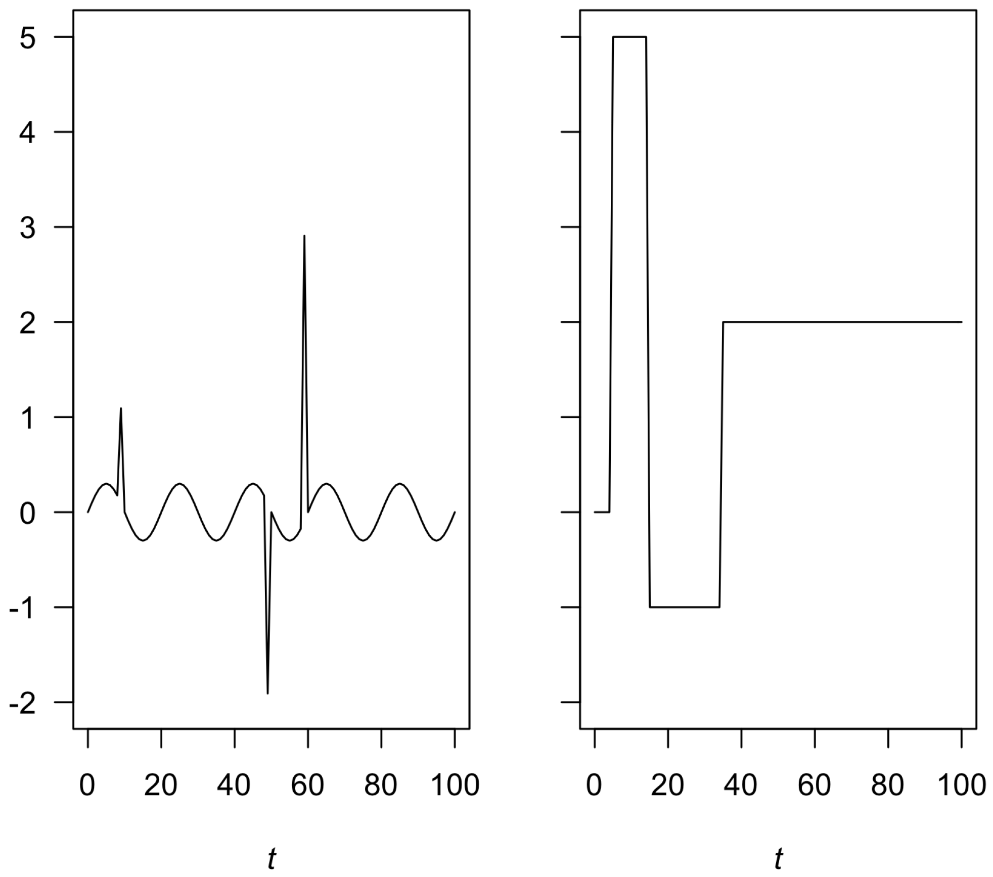
, where the functional part of the model was determined according to
that is, a sinusoidal curve with jumps at
,
and
.
The left panel of
Figure 1 shows the functional part with the three peaks described above and the right panel depicts randomly simulated mean values for the four segments.
For each series, segments were simulated, and each of them took a random value to simulate its mean value of the set {0,1,2,3,4,5}, so that they did not repeat at adjacent intervals. The positions of the change points were randomly selected, where the minimum size in each segment was of five, and the position with respect to the peaks was at a distance of at least three. In each simulation, the value of the standard deviation was constant. To evaluate the performance of the model at different noise levels, we considered the values .
For the algorithm, we considered a dictionary of over 120 functions, including Haar functions [
29] of the form
, where
and Fourier functions of the form
and
, with
, and polynomial functions of the form
t,
and constant.
The hyperparameters and were set to 50. In each iteration, it was proposed to change two change points and two in the selection of functions. To start the algorithm, we started with three segments and functions from the dictionary. The threshold for the cutoff probability in the decision to consider or not as a change point was set to , as for the selection of the dictionary functions.
To evaluate the performance of the algorithm in the simulated series, the root mean square error
was calculated for the detected change points:
For the functional part, we obtained the RMSE of the distance between the true function and the estimated one:
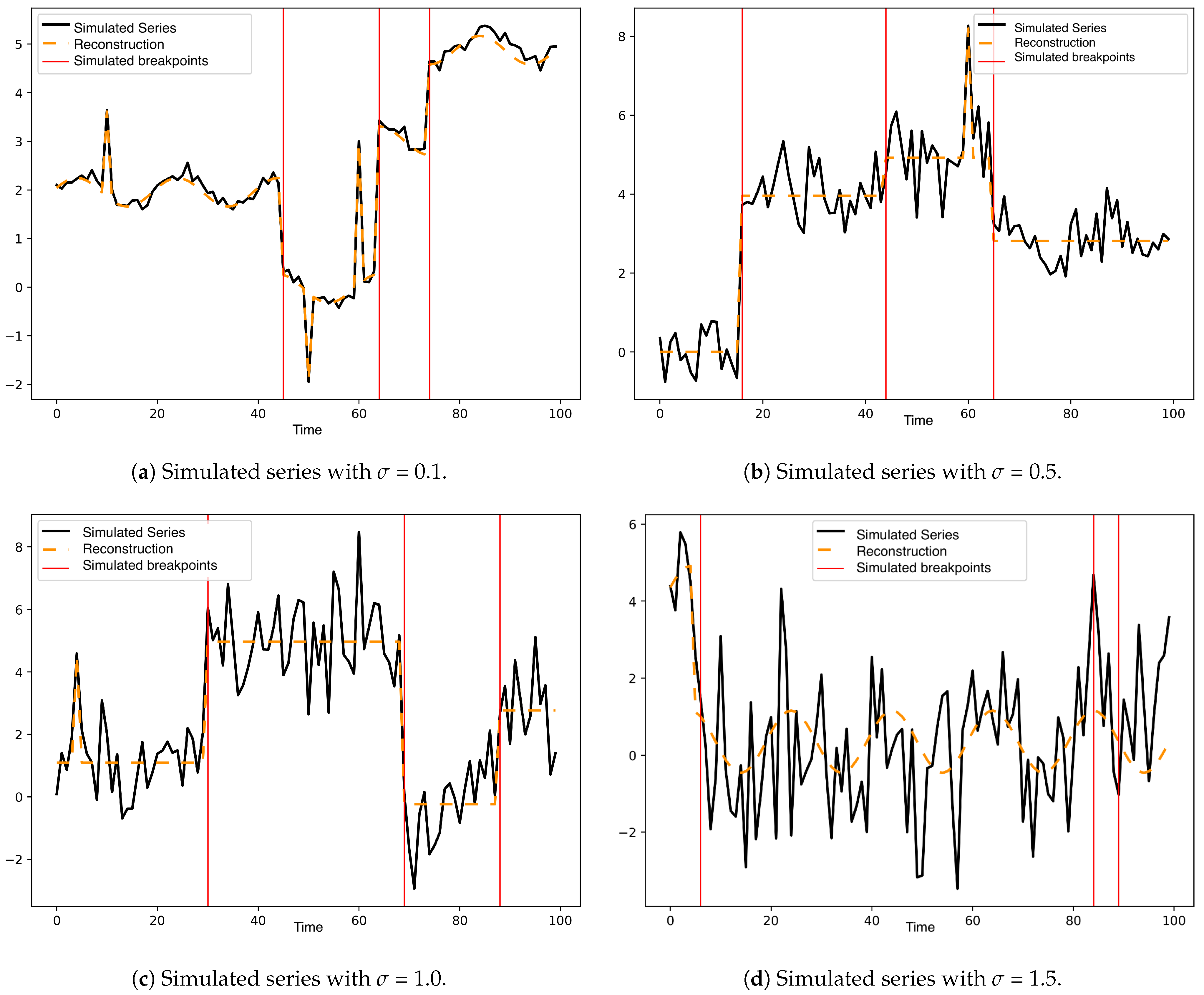
Figure 2 shows a simulated series of the 100 generated for each variance. Simulated change points were included in each image as red lines and fitted curve as segmented lines.
Figure A1 and
Figure A2 of
Appendix A show two additional simulated series for each noise level used (
in {
}) with the adjusted model.
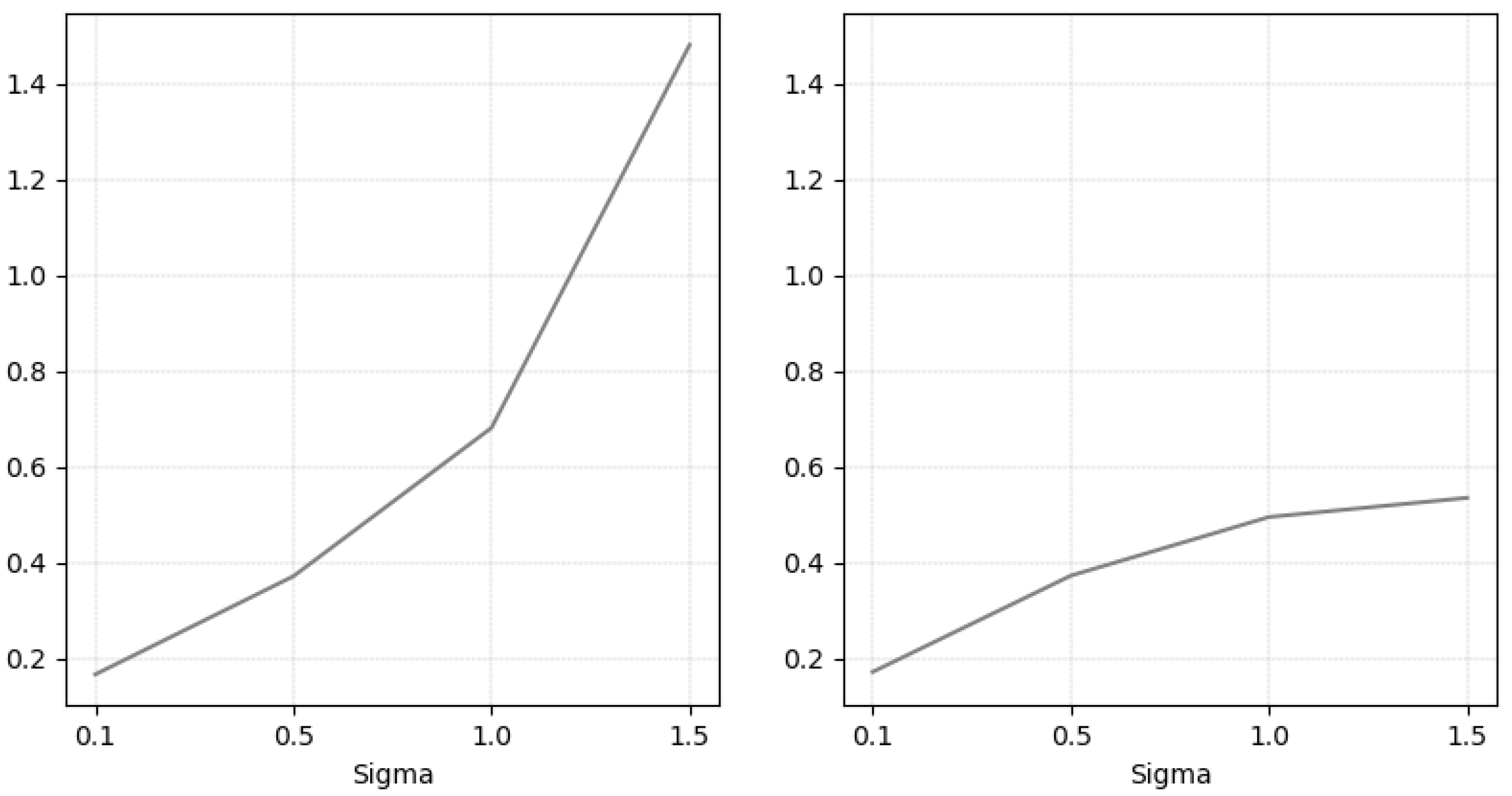
The average RMSE values for the change points and the functions are shown in
Figure 3. As expected, we observe how the error increases as the series has greater variability, which occurs in both cases.
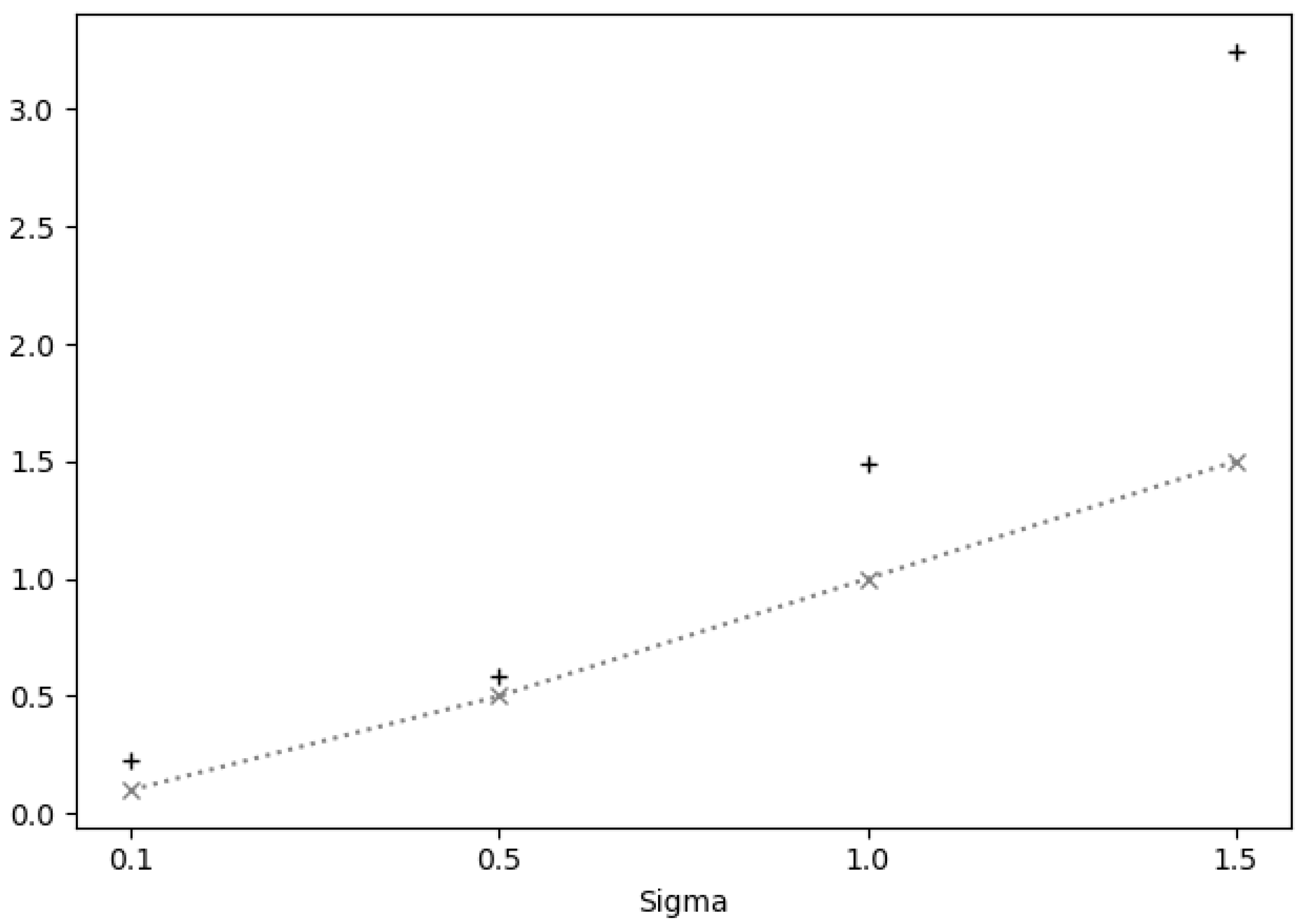
To analyze how far our estimates are from the true simulated values for the 100 series, standard deviations were averaged for each level of
used. Here, it is noteworthy that for
in
we had
reasonable average estimates of
and
, respectively; however, for
the estimates were too high, with averages of
and
, respectively (see
Figure 4).
4. Application to the USD/CLP Dataset
The USD/CLP series under study considers the dates included between January 2018 and September 2020 (available in
http://www.bcentral.cl, accessed on 23 January 2021) with daily frequency, with a total of
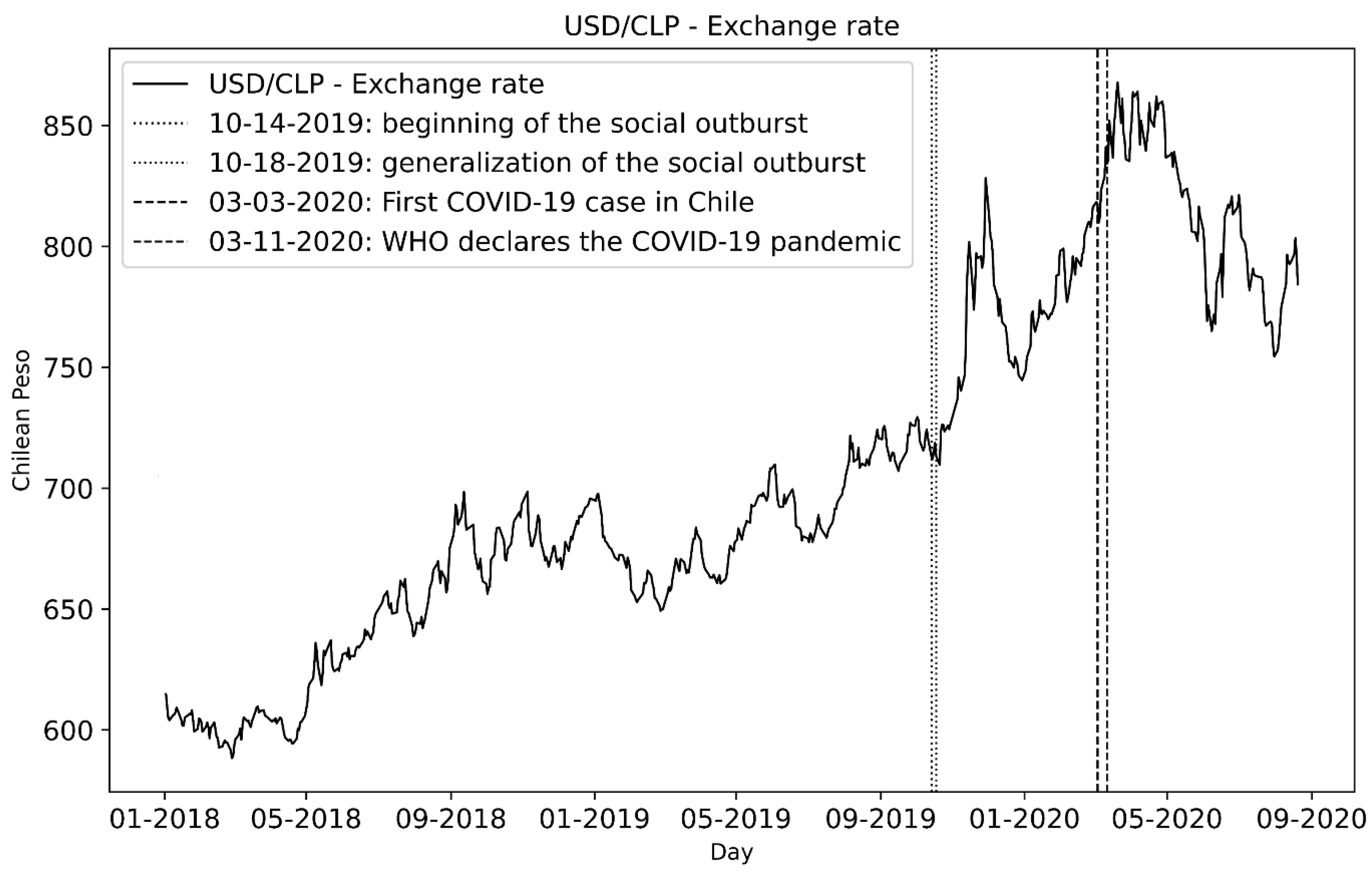
records. This series is shown in
Figure 6, highlighting the important dates that refer to the onset of the social crisis and COVID-19 pandemic events.
For the implementation of the model, we considered a dictionary with
functions, including Haar functions [
29], Fourier functions, second-degree polynomials and B-Splines [
30]. The order of the dictionary is detailed in
Table 1. In
Table 2, we summarize the constants used to analyze the USD/CLP dataset.
The methodology considered first the detection of change points without prior knowledge, expressed with a uniform probability of for each point in the series and also using different values of prior probabilities () to suggest that 14 October 2019 (the onset of the social protests in Chile) and 3 March 2020 (when the first COVID-19 case was detected in Chile) should be identified as change points.
4.1. USD/CLP without Prior Knowledge
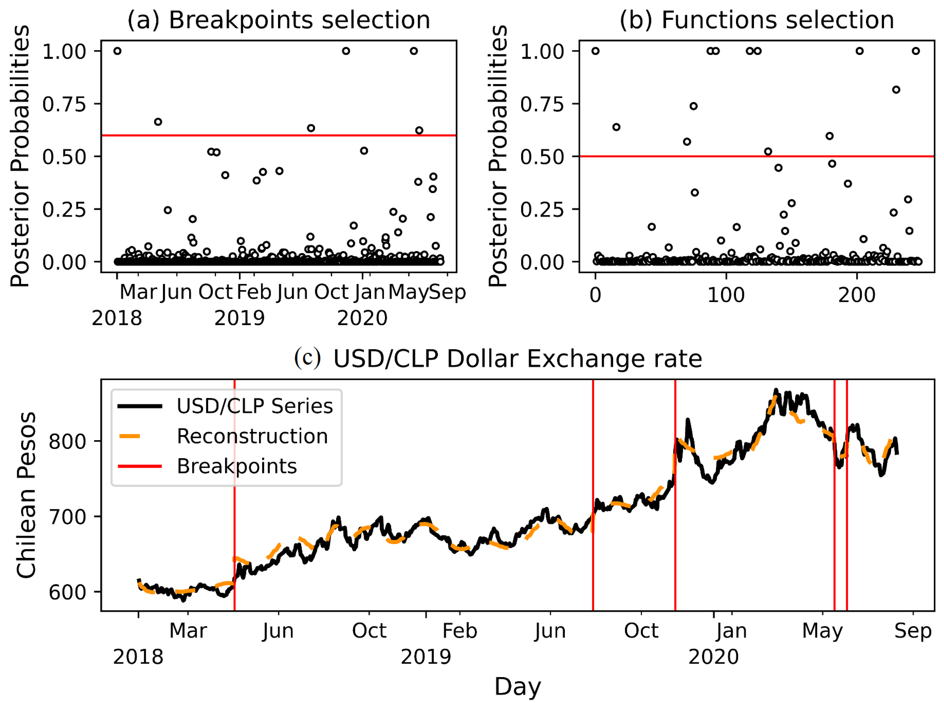
Figure 7 shows results obtained using the same prior probability
for all the points of the series, where
for all
M functions, and considering a threshold of
and
for the posterior probabilities of the selection of the change points and functions of the dictionary.
From
Figure 7, we considered five selected change points and 12 functions. The change points were on the following dates:
- 3 May 2018:
The curve shows an increase in the dollar value that differs from its previous trend. We must mention that during March 2018, the president of the United States Donald Trump announced the imposition of tariffs for USD 50 mil to products of Chinese origin, under the assumption of “unfair trade practices” and “theft of intellectual property”. After this announcement, China informed that tariffs would be applied to 128 products from the United States. Given these facts, we associate this change point with a consequence of the trade war started between China and the United States.
- 1 August 2019:
This date could be related by the beginning of the economic war between the USA and China since President Trump unveiled the 10% tariff plan on 1 August 2018, blaming China for not following through on promises to buy more American agricultural products.
- 13 November 2019:
The abrupt rise in the value of the dollar is clearly appreciated on this date. We know that on 18 October 2019 the social protests began in Chile, with the dollar reaching an observed value of Chilean pesos, and then on 29 November 2019 reaching a historical maximum of pesos. One day before the date of this change point was detected, Tuesday 12 November 2019, there was a national strike in Chile, being the day with the greatest violence registered. This day of great violence motivated the agreement for social peace and the new constitution on 15 November 2019, which is focused on the creation of a new Magna Carta, to replace the one of 1980. Consequently, this change point can be explained given the particular situation that occurred in Chile in this period.
- 2 June 2020:
At this point on the curve, we see a sharp fall in the dollar both in Chile and globally. In the Chilean case, it is mainly due to the fact that during June 2020 copper presented a significant rise due to the reopening of the US and European economies.
- 18 June 2020:
This date could be associated with the reopening of the economy in the US and Europe after going through the peak period of the COVID-19 pandemic.
4.2. Changing Prior Probabilities
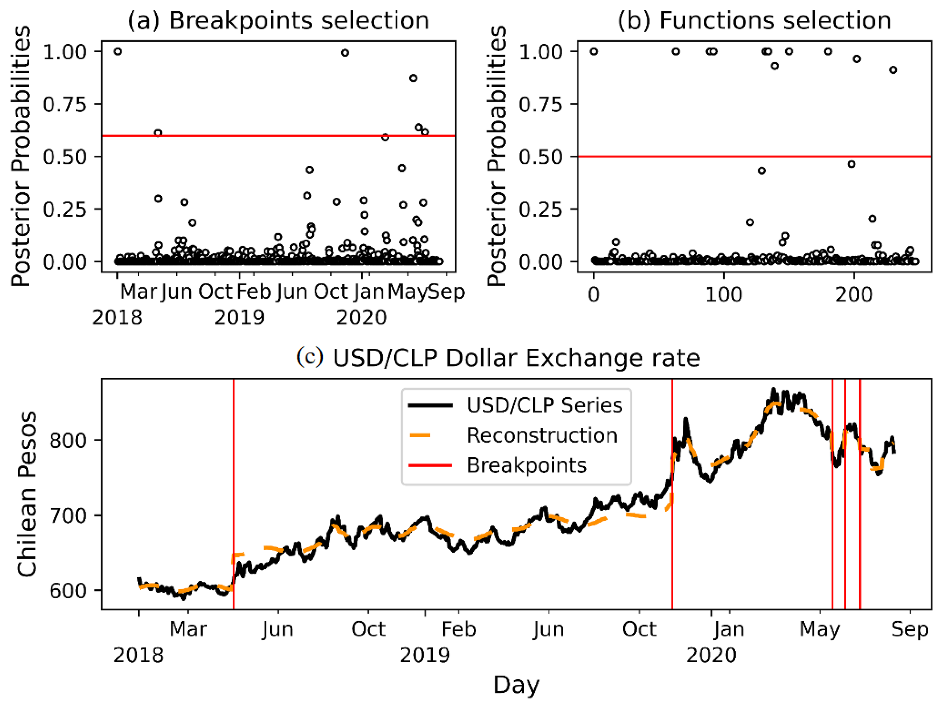
To explore the prior effect, we considered two dates: 18 October 2019, the start of the protest in Chile, and 11 March 2020, when the World Health Organization (WHO) declared the COVID-19 pandemic. For each of these dates, the prior
was set.
Figure 8 shows the results.
The change points detected corresponded to the following dates:
- 2 May 2018
We detected again this point, which is associated with the trade war between the USA and China.
- 12 November 2019
As in the case without prior knowledge, the model detected this change point, which was expected both visually and by known facts, as it corresponds to the social crisis. This time, the date on which the change point was detected is closer to the date set with prior knowledge than to the date set without prior knowledge.
- 3 June 2020
At this point, it can be seen how the model fits well to the fall in the value of the dollar, which did not occur without applying prior knowledge. This date coincides with the reopening of the economy in the US and Europe after going through the peak period of the COVID-19 pandemic.
- 18 June 2020
This date could be associated with the reopening of the economy in the US and Europe after going through the peak period of the COVID-19 pandemic.
- 8 July 2020
This date could be associated with the reopening of the economy in the US and Europe after going through the peak period of the COVID-19 pandemic.
It is important to note that two dates selected with higher probabilities, with and without prior knowledge, are related to the social crisis in Chile, 12 October 2019, and the COVID-19 pandemic, 3 June 2020.
The model which considers prior knowledge yielded an estimated variance less than that without prior knowledge on the proposed dates.
For the functional part, the model selected one Fourier function,
, one Haar function, the function
, and finally four B-splines of second order and three B-splines of third order. These results are consistent in that models with splines are widely used to approximate these types of functions. In [
31], the authors showed a model with splines to adjust the interest rate structure.
5. Discussion
The main concern of the change point problem is the complexity of building a flexible and effective model to estimate the unknown number and locations of break points in time series. In this paper, we have proposed to apply a flexible methodology in order to detect change points in the USD/CLP series in the context of social crisis and COVID-19.
For the dollar/Chilean peso time series, the model managed to detect the change points corresponding to the social protests and the start of the COVID-19 pandemic in Chile. It also suggested change points for the year 2018, dates that represented a certain beginning of the trade war between the US and China as it entered phase 2 with new tariff measures. The change points in the period of June–July 2020 coincided with the reopening of the economy in the US and Europe, after going through the first peak of COVID-19 infections.
The applied model was well adjusted for time series with small variances , which is disclosed in the simulation study. As the variance grew, we had greater errors in the detection of change points, and this was reflected in the absence of the detection of these.
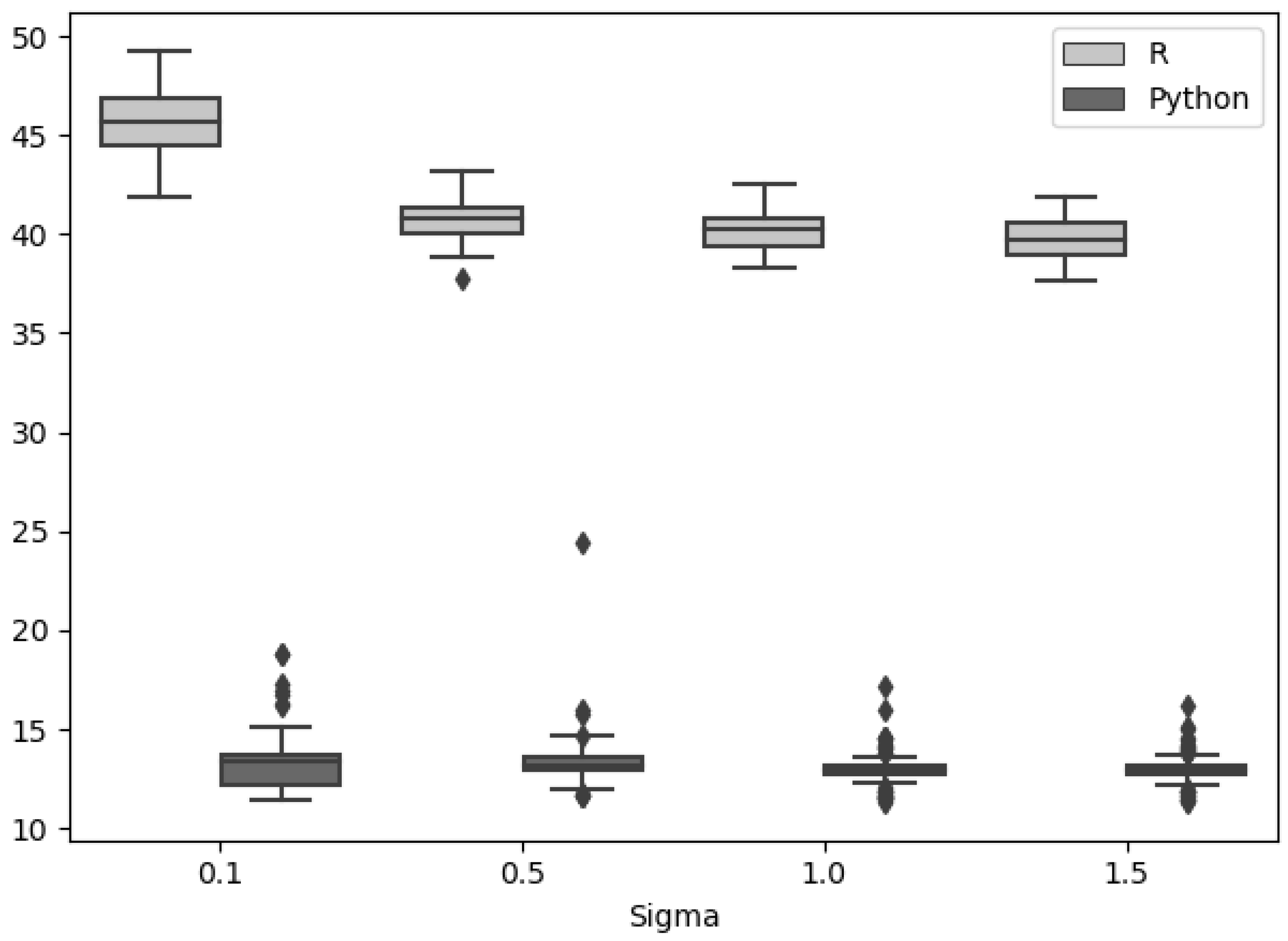
For the model, we used MCMC methods, which require long processing times. By implementing these in the Python programming language, a decrease in the average execution time of between and seconds was obtained with respect to R for the Metropolis–Hastings algorithm in simulated series with . We recommend using Python for iterative models over R.
The advantage of the Bayesian model used is that it allows us to introduce prior knowledge, which helped direct the model in the appropriate case. Another advantage is that we have the flexibility to decide the cutoff threshold to be applied, both to define what a change point will be or which dictionary function will be present.
The results suggest that the events that affected the large economies of the US and Europe affected the dollar/Chilean peso exchange rate, as the trade war between the US and China and the start of the COVID-19 pandemic led to the devaluation of the Chilean peso with respect to the dollar. When economic reactivation occurred in the US and Europe, there was also a drop in the dollar value. On the other hand, the social outburst in Chile seems to have caused a sharp rise in the value of the dollar, due to higher country risk.
Author Contributions
Conceptualization, R.d.l.C., C.M. and C.F.; methodology, C.M. and N.N.; software, N.N.; validation, R.d.l.C., C.M., N.N. and C.F.; formal analysis, C.M. and N.N.; investigation, C.M. and N.N.; resources, R.d.l.C. and C.M.; data curation, N.N.; writing—original draft preparation, R.d.l.C., C.M. and N.N.; writing—review and editing, R.d.l.C., C.M., N.N. and C.F.; visualization, C.M. and N.N.; supervision, R.d.l.C., C.M., N.N. and C.F.; project administration, C.M.; funding acquisition, R.d.l.C. and C.M. All authors have read and agreed to the published version of the manuscript.
Funding
This work was supported by the Agencia Nacional de Investigación y Desarrollo, Chile, ANID/FONDECYT/1181662 and ANID/FONDECYT/1190801.
Institutional Review Board Statement
Not applicable.
Informed Consent Statement
Not applicable.
Data Availability Statement
Acknowledgments
The authors would like to thank the reviewers for their valuable comments.
Conflicts of Interest
The authors declare no conflict of interest.
Appendix A. Settings for Some Simulated Series
Figure A1 and
Figure A2 show two simulated series for each noise level used (
in {
}) with the adjusted model.
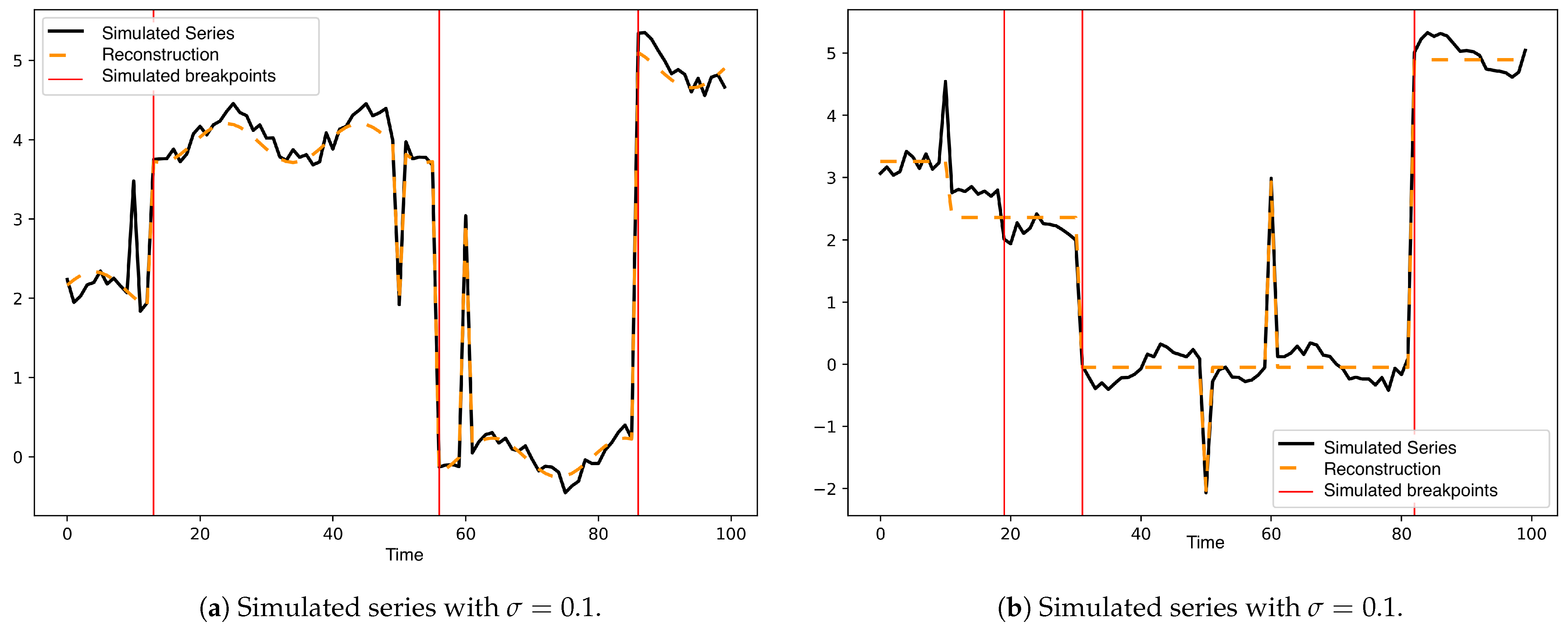
Figure A1.
In (a,b), simulated series and adjusted model for standard deviation .
Figure A1.
In (a,b), simulated series and adjusted model for standard deviation .
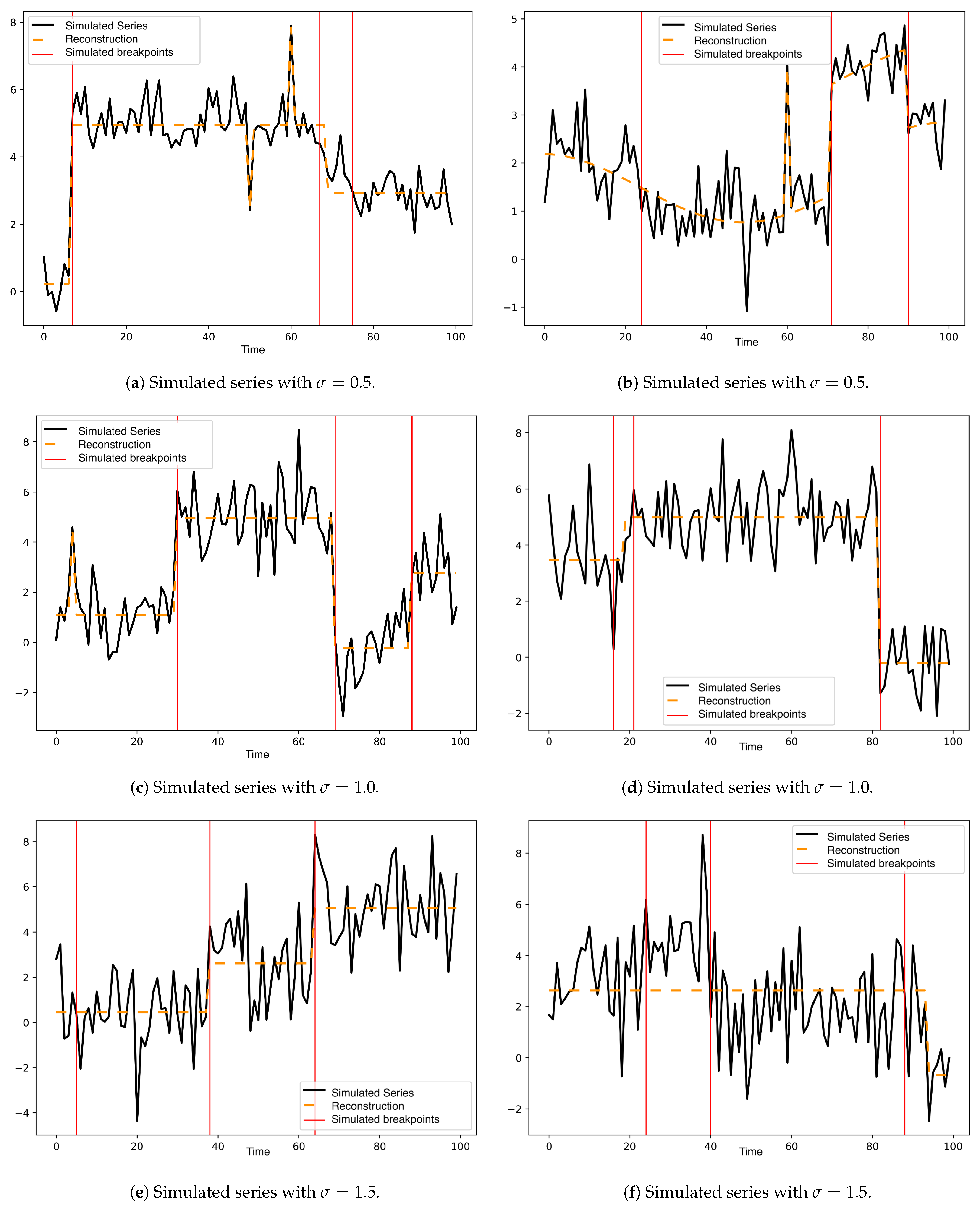
Figure A2.
In (a–f), simulated series with in {}.
Figure A2.
In (a–f), simulated series with in {}.
References
- Chowdhury, M.F.; Selouani, S.A.; O’Shaughnessy, D. Bayesian on-line spectral change point detection: A soft computing approach for on-line asr. Int. J. Speech Technol. 2012, 15, 5–23. [Google Scholar] [CrossRef]
- Ducré-Robitaille, J.-F.; Vincent, L.A.; Boulet, G. Comparison of techniques for detection of discontinuities in temperature series. Int. J. Climatol. 2003, 23, 1087–1101. [Google Scholar] [CrossRef]
- Bosc, M.; Heitz, F.; Armspach, J.-P.; Namer, I.; Gounot, D.; Rumbach, L. Automatic change detection in multimodal serial mri: Application to multiple sclerosis lesion evolution. NeuroImage 2003, 20, 643–656. [Google Scholar] [CrossRef]
- Thies, S.; Molnár, P. Bayesian change point analysis of bitcoin returns. Financ. Res. Lett. 2018, 27, 223–227. [Google Scholar] [CrossRef]
- van den Burg, G.J.; Williams, C.K. An evaluation of change point detection algorithms. arXiv 2020, arXiv:2003.06222. [Google Scholar]
- Baragatti, M.; Bertin, K.; Lebarbier, E.; Meza, C. A Bayesian approach for the segmentation of series with a functional effect. Stat. Model. 2019, 19, 194–220. [Google Scholar] [CrossRef]
- Picard, F.; Lebarbier, E.; Hoebeke, M.; Rigaill, G.; Thiam, B.; Robin, S. Joint segmentation, calling, and normalization of multiple CGH profiles. Biostatistics 2011, 12, 413–428. [Google Scholar] [CrossRef]
- Bertin, K.; Collilieux, X.; Lebarbier, E.; Meza, C. Semi-parametric segmentation of multiple series using a dp-lasso strategy. J. Stat. Comput. Simul. 2017, 87, 1255–1268. [Google Scholar] [CrossRef]
- Sharma, S.; Swayne, D.A.; Obimbo, C. Trend analysis and change point techniques: A survey. Energy Ecol. Environ. 2016, 1, 123–130. [Google Scholar] [CrossRef]
- Ruggieri, E.; Antonellis, M. An exact approach to bayesian sequential change point detection. Comput. Stat. Data Anal. 2016, 97, 71–86. [Google Scholar] [CrossRef]
- Aminikhanghahi, S.; Cook, D.J. A survey of methods for time series change point detection. Knowl. Inf. Syst. 2017, 51, 339–367. [Google Scholar] [CrossRef] [PubMed] [Green Version]
- Truong, C.; Oudre, L.; Vayatis, N. Selective review of offline change point detection methods. Signal Process. 2020, 167, 107299. [Google Scholar] [CrossRef]
- Jiang, F.; Zhao, Z.; Shao, X. Time series analysis of covid-19 infection curve: A change-point perspective. J. Econom. 2020. [Google Scholar] [CrossRef] [PubMed]
- Zhang, S.; Xu, Z.; Peng, H. Change point modeling of COVID-19 data in the united states. Stat. Appl. 2021, 18, 307–318. [Google Scholar]
- Jegede, S.L.; Szajowski, K.J. Change-point detection in homogeneous segments of COVID-19 daily infection. Axioms 2022, 11, 213. [Google Scholar] [CrossRef]
- Lavielle, M.; Lebarbier, E. An application of MCMC methods for the multiple change-points problem. Signal Process. 2001, 81, 39–53. [Google Scholar] [CrossRef]
- Boys, R.J.; Henderson, D.A. A bayesian approach to dna sequence segmentation. Biometrics 2004, 60, 573–581. [Google Scholar] [CrossRef]
- Erdman, C.; Emerson, J.W. A fast Bayesian change point analysis for the segmentation of microarray data. Bioinformatics 2008, 24, 2143–2148. [Google Scholar] [CrossRef]
- R Core Team. R: A Language and Environment for Statistical Computing; R Foundation for Statistical Computing: Vienna, Austria, 2020. [Google Scholar]
- Rossum, G.V.; Drake, F.L. Python 3 Reference Manual; CreateSpace: Scotts Valley, CA, USA, 2009. [Google Scholar]
- Harchaoui, Z.; Lévy-Leduc, C. Multiple change-point estimation with a total variation penalty. J. Am. Stat. Assoc. 2010, 105, 1480–1493. [Google Scholar] [CrossRef]
- Edward, G.; McCulloch, R. Variable selection via gibbs sampling. J. Am. Stat. Assoc. 1993, 88, 881–889. [Google Scholar]
- Casella, G.; George, E.I. Explaining the gibbs sampler. Am. Stat. 1992, 46, 167–174. [Google Scholar]
- Chib, S.; Greenberg, E. Understanding the metropolis-hastings algorithm. Am. Stat. 1995, 49, 327–335. [Google Scholar]
- Zellner, A. On assessing prior distributions and bayesian regression analysis with g-prior distributions. Bayesian Inference Decis. Tech. 1986, 6, 233–243. [Google Scholar]
- Garcia-Donato, G.; Forte, A.; Steel, M. Methods and tools for bayesian variable selection and model averaging in normal linear regression. Int. Stat. Rev. 2018, 86, 237–258. [Google Scholar]
- Ley, E.; Fernández, C.; Steel, M.F.J. Benchmark priors for bayesian model averaging. J. Econom. 2001, 100, 381–427. [Google Scholar]
- Christensen, M.G.; Cemgil, A.T.; Nielsen, J.K.; Jensen, S.H. Bayesian model comparison with the g-prior. IEEE Trans. Signal Process. 2014, 62, 225–238. [Google Scholar]
- Härdle, W.; Kerkyacharian, G.; Picard, D.; Tsybakov, A. Wavelets; Springer: New York, NY, USA, 1998; pp. 1–16. [Google Scholar]
- Eilers, P.H.C.; Marx, B.D. Flexible smoothing with b-splines and penalties. Stat. Sci. 1996, 11, 89–102. [Google Scholar] [CrossRef]
- Rodriguez, F.F. Interest rate term structure modeling using free knot splines. J. Bus. 2006, 79, 3083–3099. [Google Scholar] [CrossRef]
Figure 1.
Left panel: simulated functional part for the peaks and . Right panel: example for randomly simulated means, considering the constraints of distance of at least three to the peaks and a minimum length of five.
Figure 1.
Left panel: simulated functional part for the peaks and . Right panel: example for randomly simulated means, considering the constraints of distance of at least three to the peaks and a minimum length of five.
Figure 2.
In (a–d), one of the 100 series is shown for each standard deviation in including the adjusted curve.
Figure 2.
In (a–d), one of the 100 series is shown for each standard deviation in including the adjusted curve.
Figure 3.
RMSE for in . Left panel: RMSE(). Right panel: RMSE for the functions.
Figure 3.
RMSE for in . Left panel: RMSE(). Right panel: RMSE for the functions.
Figure 4.
Average of the estimates (“+” symbol) for different levels of standard deviations in used in the simulation of the 100 series. The true value is represented by the “x” symbol.
Figure 4.
Average of the estimates (“+” symbol) for different levels of standard deviations in used in the simulation of the 100 series. The true value is represented by the “x” symbol.
Figure 5.
Execution times in seconds (in the y axis), using R (in light gray) and Python (dark gray), for standard deviations in for the 100 simulated series.
Figure 5.
Execution times in seconds (in the y axis), using R (in light gray) and Python (dark gray), for standard deviations in for the 100 simulated series.
Figure 6.
Dollar/Chilean peso series. The start dates of the social outburst and COVID-19 pandemic are indicated in vertical dashed lines.
Figure 6.
Dollar/Chilean peso series. The start dates of the social outburst and COVID-19 pandemic are indicated in vertical dashed lines.
Figure 7.
Top: Posterior probabilities for selection of change points (a) and functions (b) without prior knowledge. Bottom: (c) Estimated expectation and change points.
Figure 7.
Top: Posterior probabilities for selection of change points (a) and functions (b) without prior knowledge. Bottom: (c) Estimated expectation and change points.
Figure 8.
Top: Posterior probabilities for selection of change points (a) and functions (b) with a prior probability of for the onset of social protests and the declaration of COVID-19 as world pandemic by the World Health Organization, for the segmentation part. Bottom: (c) Estimated expectation and change points.
Table 1.
Details of the 248-function dictionary applied to the dollar/Chilean peso series.
Table 1.
Details of the 248-function dictionary applied to the dollar/Chilean peso series.
| Index | Function |
|---|
| 1 | |
| 2 | Haar function in |
| ⋮ | ⋮ |
| 65 | Haar function in |
| 66 | |
| 67 | |
| ⋮ | ⋮ |
| 90 | |
| 91 | |
| 92 | t |
| 93 | |
| 94 | B-Splines order 1, with 1 node |
| ⋮ | ⋮ |
| 124 | B-Splines order 1, with 30 nodes |
| 125 | B-Splines order 2, with 1 node |
| ⋮ | ⋮ |
| 154 | B-Splines order 2, with 31 nodes |
| 155 | B-Splines order 3, with 1 node |
| ⋮ | ⋮ |
| 186 | B-Splines order 3, with 32 nodes |
| 187 | B-Splines order 4, with 1 node |
| ⋮ | ⋮ |
| 248 | B-Splines order 4, with 62 nodes |
Table 2.
Constants used for model execution.
Table 2.
Constants used for model execution.
| Constants | Value |
|---|
| Iteration number | 160,000 |
| First simulated values (burn-in) | 40,000 |
| and | 50 |
| Number of initial segments | 5 |
| Number of initial dictionary functions | 5 |
| Number of proposed change points in each iteration | 1 |
| Number of dictionary functions proposed in each iteration | 1 |
| Publisher’s Note: MDPI stays neutral with regard to jurisdictional claims in published maps and institutional affiliations. |
© 2022 by the authors. Licensee MDPI, Basel, Switzerland. This article is an open access article distributed under the terms and conditions of the Creative Commons Attribution (CC BY) license (https://creativecommons.org/licenses/by/4.0/).


