A Cooperative Control Algorithm for Line and Predecessor Following Platoons Subject to Unreliable Distance Measurements

Abstract

This paper uses a line-following approach to study the longitudinal and lateral problems in vehicle platooning. Under this setup, we assume that inter-vehicle distance sensing is unreliable and propose a cooperative control strategy to render the platoon less vulnerable to these sensing difficulties. The proposed control scheme uses the velocity of the predecessor vehicle, communicated through a Vehicle-to-Vehicle technology, to avoid significant oscillations in the local speed provoked by tracking using unreliable local distance measurements. We implement the proposed control algorithm in the RUPU platform, a low-cost experimental platform with wireless communication interfaces that enable the implementation of cooperative control schemes for mobile agent platooning. The experiments show the effectiveness of the proposed cooperative control scheme in maintaining a suitable performance even when subject to temporal distortions in local measurements, which, in the considered experimental setup, arise from losing the line-of-sight of the local sensors in paths with closed curves.

1. Introduction

In Cooperative Adaptive Cruise Control (CACC) applications, a platoon of vehicles coordinates its actions to navigate along a predefined path while maintaining the desired distance between vehicles [1,2,3]. Considering a platoon of vehicles traveling on a highway, the collective behavior can be achieved through the local control of each vehicle based on its own perception of the environment but also with information received from other vehicles through Vehicle-to-Vehicle (V2V) and Vehicle-to-Infrastructure (V2I) [4] communication. Vehicle platooning applications are expected to provide a backbone for future Intelligent Transportation Systems (ITS) technologies [5], bringing significant improvements in safety, congestion management, energy efficiency, reduction of emissions, etc. [6,7,8].

In practical scenarios representative of urban roads and highways, the drivable sections are marked with lanes delimited with painted lines. Each vehicle is then required to detect the lanes and determine its relative position and orientation with respect to the lanes to calculate a smooth path to traverse while staying within the delimited drivable region. Extending the scenario to a platoon configuration introduces the requirement for each vehicle to maintain a predefined distance from its predecessor. With the previous considerations, the control problem of path-following platooning can be seen as a dual problem [9]: (i) the lateral problem, which requires each vehicle to move along a predefined path [10]; and (ii) the longitudinal problem, which requires each vehicle to maintain a predefined distance from its predecessor [11]. Simultaneously addressing both control problems for each vehicle is challenging since achieving one goal may harm the other due to the coupled dynamics. This interplay between control objectives is receiving attention in the context of individual autonomous vehicles [12,13,14] and, more recently, in platooning [15,16,17].

Path-following applications are typically preceded by a path-planning stage in which each vehicle defines a trajectory to move smoothly along the delimited region of the road [18,19]. This requires each vehicle to be equipped with sensors and computing capabilities to perceive the lane ahead and disturbances such as obstacles or changes in road conditions. The rapid proliferation of technologies associated with Advanced Driving Assistance Systems (ADASs) has pushed the development of multiple techniques for lane-keeping and optimal path-planning, which generally project the path to follow using a single virtual line along the center of the lane. Nowadays, autonomous vehicle path-planning algorithms remain an active research topic [19,20,21], and there are also commercial solutions already available in modern cars [22,23]. In the case of platoon formations, each vehicle can address the lateral problem by either implementing its own lane-keeping system or following the state of the leading vehicle; however, additional challenges arise due to the coupling with the longitudinal problem.

A fundamental aspect of safe vehicular navigation is the reliability of environment perception [24]. Control algorithms for path-following platoons rely on an appropriate measure of the inter-vehicle distances. In practice, distance sensing could be unreliable due to, for example, the inaccuracy of sensing devices [25], the effect of turns that may affect the path-planning stage yielding cutting-corner phenomena [16], and temporal interference in the line of sight of the ranging sensors due to curves, inclinations, and obstacles in the road [26]. The latter case is critical for distance tracking since the vehicle cannot detect the predecessor. Although unreliable distance measurement is part of the underlying platooning navigation problem in a natural environment, it remains a mostly unexplored research topic in path-following platooning control. Most of the related research is focused on collision avoidance [27], string stabilization [28,29], which is also relevant for smooth navigation, and recently on communication issues in the network that connects vehicles, such as noisy channels or data dropouts, [30,31]. Strategies that deal with these problems may help to cope with intermittent distance measurement loss.

On the other hand, evaluating control algorithms for platooning considering curved paths, non-reliable communication, and other challenges requires testing them in real scenarios where non-modeled interactions may arise, especially for large formations. Major commercial conglomerates have implemented and tested platooning configurations using real-scale vehicles and road infrastructure [32]. However, these experiments are targeted as industrial technological demonstrators, and the data and results are not openly available for scrutiny and academic research. Moreover, the high costs of these experiments preclude experimental research on new control algorithms for large platoons. A suitable alternative for experimental evaluation is the use of scaled-down platforms that capture the essence and challenges of control problems in path-following platooning, allowing for quick and safe testing of new control algorithms.

In this paper, we introduce the approach of line-following platooning to study the fundamental control problems arising in path-following platooning. In this approach, we assume that the navigation is carried on an established road and that the path-planning stage in each vehicle is properly working, such that the target path can be represented through a single line painted on the floor. The proposed framework avoids the required hardware and software necessary for lane detection and path planning in an experimental setup while still capturing the essence of the underlying longitudinal and lateral control problems, allowing us to observe and study relevant aspects of platooning such as string stability, cooperative schemes, and sensing and communication challenges. We use this approach to evaluate a line-following platoon with a predecessor-following communication topology, i.e., each vehicle has access to its own information but also some data from its predecessor obtained via V2V communication. The main contribution of this paper is the proposal and experimental evaluation of a cooperative control algorithm to deal with both lateral and longitudinal problems in line-following platooning where local measurements of inter-vehicle distance are unreliable. The control algorithm consists of a set of controllers in a multi-input multi-output (MIMO) scheme, enhanced by a non-linear function that limits the vehicle speed based on that of the predecessor. We test the proposed algorithm using the RUPU experimental platform, consisting of a set of scaled-down vehicles with wireless communication interfaces that we specifically designed to study platooning problems. Experimental results using the proposed cooperative control scheme show that the platoon is less vulnerable to unreliable distance measurements when contrasted with its non-cooperative counterpart.

The rest of the paper is organized as follows: Section 2 presents the line-following platooning control problem. The RUPU experimental platform is described in Section 3, while the proposed control algorithm is in Section 4. Section 5 presents the experimental results obtained from the case studies, and Section 6 summarizes the conclusions and future work.

2. The Line-Following Platooning Control Problem

Modern ADASs in commercial self-driving vehicles implement path-planning algorithms that project the path to follow as a virtual line along the road [23]. In this work, we assume that the platoon navigates on an established road with properly marked lanes and that the path-planning stage in each vehicle provides a single line to follow. Isolating the path-planning stage from the main control problems simplifies the analysis and evaluation of the platooning formation, reducing the more general path-following platooning problem to a line-following platooning configuration. At the same time, the configuration still retains the essence and challenges associated with the lateral and longitudinal control problems. The proposed approach presents the following advantages:

• Individual vehicles may adapt existing techniques from line-following robot literature to help deal with the lateral problem (see e.g., [33,34]).
• Despite the simplification in the setup, the configuration retains fundamental challenges that arise in control of platoon formations, such as dealing with unreliable distance measurement, designing string stabilizing controllers, and considering communication issues, among others.
• The decoupling of the path-planning stage relieves the mathematical treatment from analytically studying platooning for more than one-dimensional paths, allowing to concentrate on the primary control problems.
• Enables the development of low-cost experimental platforms to evaluate platooning formations using low-cost sensors for line-following applications (e.g., infrared sensors), without requiring sophisticated hardware and software support for cameras or lidars that are normally required for the path-planning stage [16,20].

Indeed, considering the growing interest in ITS technology, the infrastructure must be adapted to support autonomous navigation at a large scale. In this context, it is reasonable to assume that roads will have predefined marked lines and signaling to facilitate platooning and autonomous navigation in a similar fashion to the proposed line-following configuration.

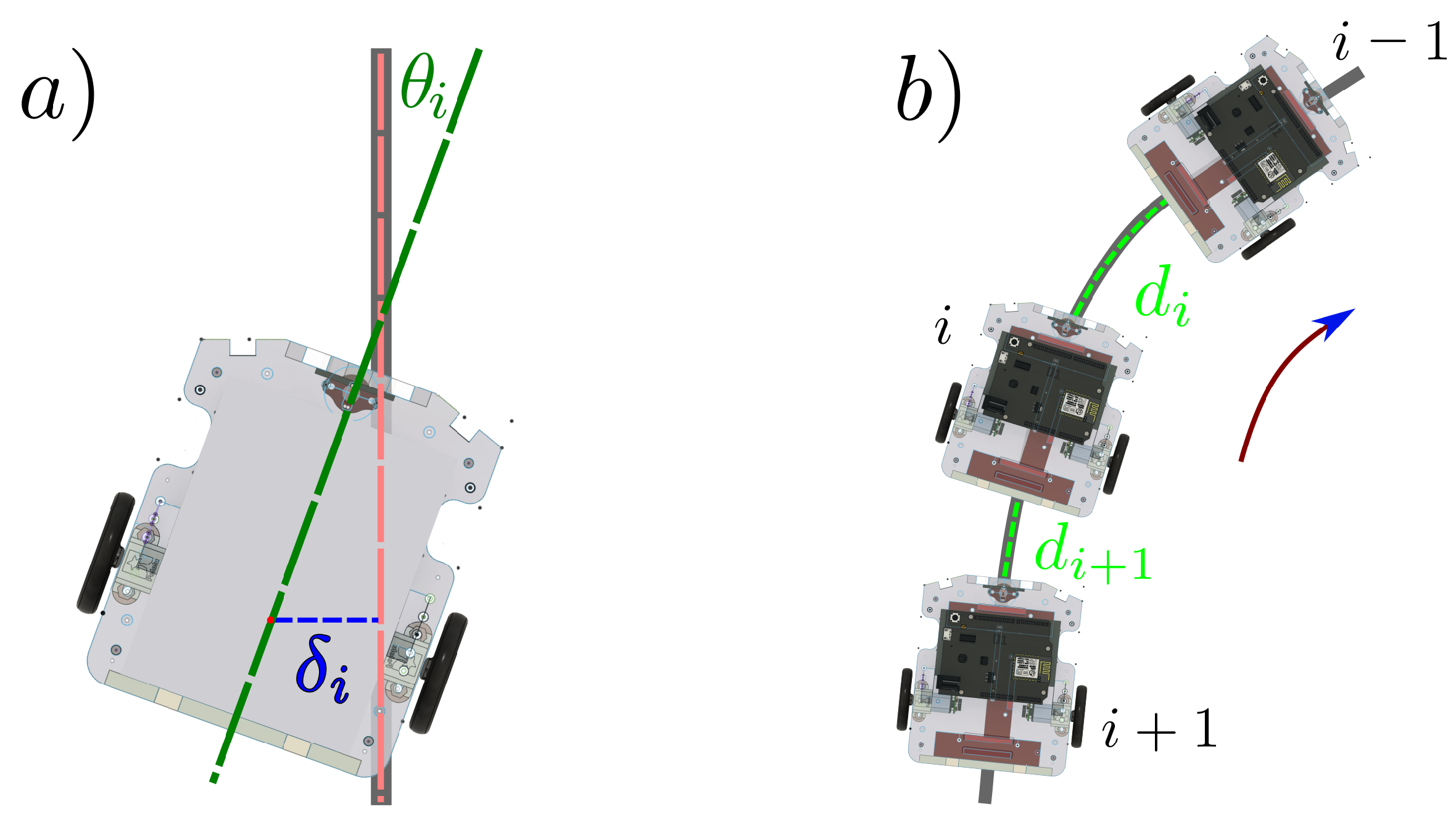
Figure 1 shows a representation of the variables involved in both lateral and longitudinal control problems arising in line-following platoons. The figures consider the example of a vehicle identified with the index i, with $i=1,\cdots N-1$, where N is the total number of vehicles in the platoon. The vehicle with index $i=0$ represents the platoon leader. Figure 1a represents the lateral control problem for vehicle i. This setup requires each vehicle to determine its position and orientation with respect to the reference line and, based on such information, to position itself in the desired way on the road. The red dashed line represents the desired path along the road, ${\delta }_i\left(t\right)$ denotes the perpendicular distance from the line to be followed to the middle point of the wheel axle, and the angle ${\theta }_i\left(t\right)$ represents the orientation respect to the desired moving direction. An appropriate position for navigation is when both ${\delta }_i\left(t\right)$ and ${\theta }_i\left(t\right)$ are close to zero. Figure 1b represents the longitudinal control problem for a set of vehicles. The distance between vehicle i and its predecessor $i-1$ is denoted by $d_i\left(t\right)$. Note that we represent the inter-vehicle distance as the shortest path between the front part of a vehicle and the rear of the preceding vehicle along the reference line to follow. Here, the goal is to achieve $d_i\left(t\right)=r_i\left(t\right)$, where $r_i\left(t\right)$ is a given desired distance.

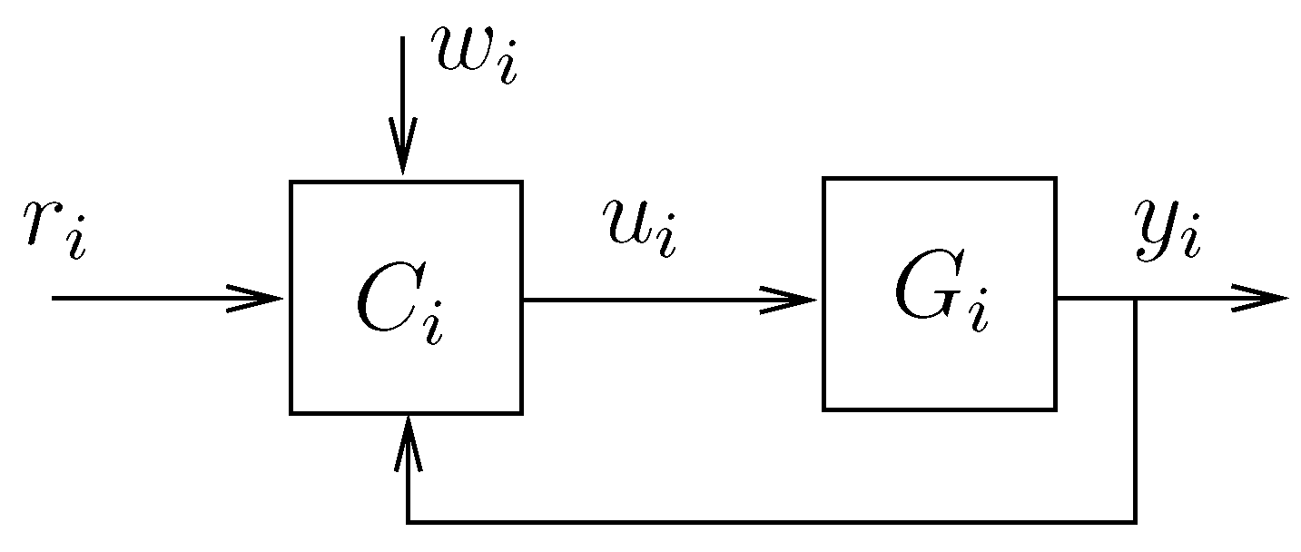
The overall platooning control scheme requires simultaneously addressing both the lateral and the longitudinal problems. So, we can view each vehicle as a multi-input, multi-output (MIMO) feedback control system [35]. Figure 2 shows a general diagram of the control loop, where $G_i$ represents the MIMO dynamical model of the vehicle, $C_i$ is the MIMO controller, $r_i\left(t\right)$ denotes the desired inter-vehicle distance, $w_i\left(t\right)$ represents a vector with the information obtained from other vehicles, $z_i\left(t\right)$ is a vector with the variables to be controlled, that is, ${\theta }_i\left(t\right)$, ${\delta }_i\left(t\right)$ and $d_i\left(t\right)$, and $u_i\left(t\right)$ is a control signal that manipulates the steering, acceleration, and braking of the vehicle. When each vehicle is initially positioned on the line, an appropriate controller design should perform so that ${\delta }_i\left(t\right)\approx 0$ most of the time. Thus, considering an initial routine to position each agent on the line path, it is reasonable to assume that ${\delta }_i\left(t\right)=0$ and the problem reduces to controlling both ${\theta }_i\left(t\right)$ and $d_i\left(t\right)$.

The general feedback control system in Figure 2 can be tailored to deal with specific frameworks, such as considering different linear or non-linear controllers and dynamical models. We could assume the desired distance $r_i\left(t\right)$ to be constant or time-variant, allowing the inclusion of time headway policies for inter-vehicle distance [28]. Furthermore, we can study the control problem in continuous-time, discrete-time, or frequency domains. We could also consider that each controller uses only local information (i.e., $w_i\left(t\right)=0$) or a cooperative framework in which the vehicles exchange data via V2V communication, which would require specifying a network topology [36]. Several communication topologies can be explored, with one of the most common being the one in which each vehicle shares some information with its immediate follower (predecessor–follower topology) [37].

We consider that the whole platoon is governed in a distributed but coordinated fashion through the local MIMO controllers in each vehicle. We do not consider the case where a single control unit uses the information of the whole platoon and computes the control signals for every vehicle in a centralized manner. Although such centralized control approach is normally expected to perform better than the distributed approach, it is not representative of real-world platooning scenarios, where each vehicle is autonomous and locally controlled.

For the control problem, the primary goal of each vehicle is to keep the tracking error signal $e_i\left(t\right)$ close to zero most of the time. The error is defined by

$$e_i\left(t\right)=\left[\begin{array}{c}{e}_{d_i}\left(t\right)\\ e_{{\theta }_i}\left(t\right)\end{array}\right]=\left[\begin{array}{c}{r}_i\left(t\right)-d_i\left(t\right)\\ {\theta }_i\left(t\right)\end{array}\right].$$

(1)

The essential requirement is the design of stabilizing MIMO controllers and achieving zero steady-state error for each vehicle. Additional properties such as string stability and robustness against unreliable sensor measurements are important research topics.

In this paper, we propose a cooperative control algorithm for line-following platooning with unreliable distance measurements. To focus on the relevant aspects of the control problems, we assume a predecessor–follower topology and that vehicles communicate through an ideal communication channel. We validate the proposed approach using an experimental platform whose capabilities and dynamical model are described next.

3. Description of the RUPU Platform

The RUPU platform is a novel experimental platform that comprises two elements: (i) a surface with a customizable path to follow and (ii) a set of electromechanical mobile agents equipped with sensing and computing hardware necessary to follow the line in the path and track its immediate predecessor with a desired safety distance. We have designed and built the RUPU platform specifically to study platooning and multiagent problems. Figure 3 shows a general overview of a sample surface and three mobile agents.

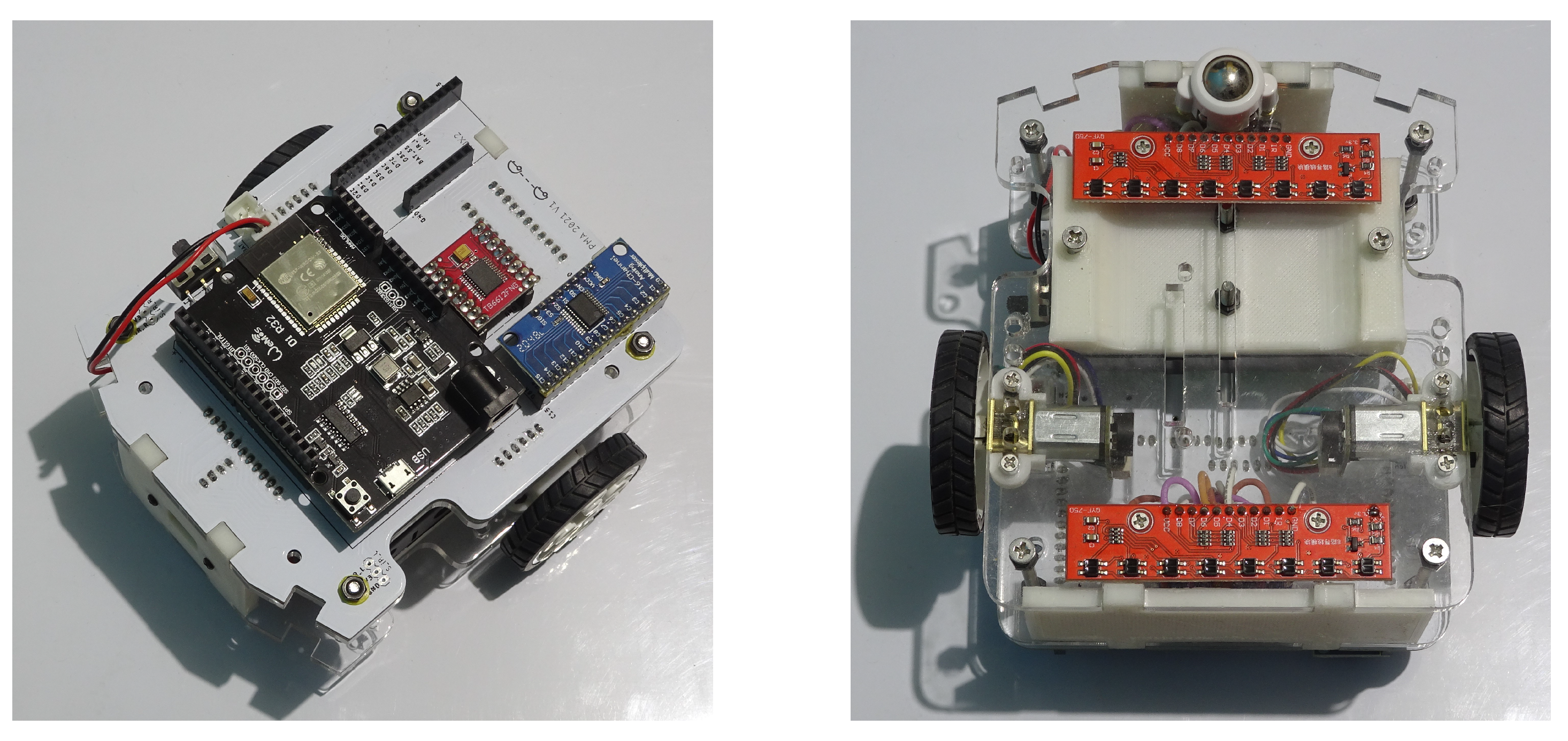
Each agent is implemented as a differential drive mobile robot (DDMR) that can move autonomously through two active wheels, which are controlled independently to allow agents to move forward, backward, rotate, turn, or maintain a curved trajectory. Regarding sensing capabilities, each agent is equipped with a time-of-flight distance sensor located in the front, which allows the vehicle to measure the distance from the front of the agent to some object ahead. The orientation of each agent with respect to the white line in the path is measured with two arrays of eight infrared sensors located at the bottom of each agent. The infrared sensors allow for determining if the line is below the agent and measuring the orientation with respect to its axis of translation. The agents can implement initialization routines to get themselves aligned with the line to follow before performing experiments. Finally, the speed of the agents is measured through two Hall-effect encoders located within each DC motor, which collect data on the angular position, sense of rotation, and the rotational speed of each wheel. The central processing core for each agent is an ESP32 embedded development board, which possesses an integrated WiFi module for wireless communication. Additional user-interface devices provide support for monitoring purposes and online interaction. Figure 4 shows two views of an agent.

3.1. Dynamical Model for Control Synthesis

This section presents a simple linear dynamical model derived for each agent in the platoon moving along a straight line. To ease notation, in this section, we consider an arbitrary agent and omit the index i referring to the agent’s position within the platoon.

The agent has two control inputs, which are the right and left motors voltages, denoted by $u_{mr}\left(t\right)$, $u_{ml}\left(t\right)$, respectively. The angular positions of the right and left wheels of the agent are denoted by ${\varphi }_r\left(t\right)$, ${\varphi }_l\left(t\right)$, respectively. The signals of interest are the linear velocity $v\left(t\right)$, the position $p\left(t\right)$, and the angular position $\theta \left(t\right)$ with respect to the line, which can be modeled as

$$\begin{array}{cc}\hfill v\left(t\right)& =\frac{r}{2}\left(\dot{{\varphi }_r}\left(t\right)+\dot{{\varphi }_l}\left(t\right)\right),\hfill \end{array}$$

(2)

$$\begin{array}{cc}\hfill p\left(t\right)& =\frac{r}{2}\left({\varphi }_r\left(t\right)+{\varphi }_l\left(t\right)\right),\hfill \end{array}$$

(3)

$$\begin{array}{cc}\hfill \theta \left(t\right)& =\frac{r}{2l}\left({\varphi }_r\left(t\right)-{\varphi }_l\left(t\right)\right).\hfill \end{array}$$

(4)

Based on an Euler–Lagrange modeling considering the dynamics of the motor and the geometry of the chassis, we perform standard parameter estimation techniques (see, for instance, [38] and the references therein) to obtain the following model, which is presented in the frequency domain:

$$\begin{array}{c}\hfill \underset{Z\left(s\right)}{\underbrace{\left[\begin{array}{c}V\left(s\right)\\ P\left(s\right)\\ \mathsf{\Theta }\left(s\right)\end{array}\right]}}=\underset{G\left(s\right)}{\underbrace{\left[\begin{array}{cc}{G}_{11}\left(s\right)& G_{12}\left(s\right)\\ G_{21}\left(s\right)& G_{22}\left(s\right)\\ G_{31}\left(s\right)& G_{32}\left(s\right)\end{array}\right]}}\underset{U\left(s\right)}{\underbrace{\left[\begin{array}{c}{U}_{mr}\left(s\right)\\ U_{ml}\left(s\right)\end{array}\right]}}\end{array}$$

(5)

where $V\left(s\right)$, $P\left(s\right)$, $\mathsf{\Theta }\left(s\right)$, $U_{mr}\left(s\right)$, and $U_{ml}\left(s\right)$ are the Laplace transforms of $v\left(t\right)$, $p\left(t\right)$, $\theta \left(t\right)$, $u_{mr}\left(t\right)$, and $u_{ml}\left(t\right)$ respectively, and

$$\begin{array}{cc}\hfill G_{11}\left(s\right)& =G_{12}\left(s\right)=\frac{120020}{(s+4592)(s+7.187)},\hfill \end{array}$$

(6)

$$\begin{array}{cc}\hfill G_{21}\left(s\right)& =G_{22}\left(s\right)=\frac{120020}{s(s+4592)(s+7.187)},\hfill \end{array}$$

(7)

$$\begin{array}{cc}\hfill G_{31}\left(s\right)& =-G_{32}\left(s\right)=\frac{24962}{s(s+4591)(s+8.372)}.\hfill \end{array}$$

(8)

The structure of the transfer matrix $G\left(s\right)$ is due to the symmetry in the agent construction and also because the agent velocity is the derivative of the position, explaining the deficient rank for $G\left(s\right)$. Thus, the model is essentially a two-input, two-output model since the distance and velocity are not independent variables. Indeed, we can write

$$\begin{array}{c}\hfill G\left(s\right)=\left[\begin{array}{cc}{G}_{11}\left(s\right)& 0\\ G_{11}\left(s\right)/s& 0\\ 0& G_{31}\left(s\right)\end{array}\right]\underset{M_u}{\underbrace{\left[\begin{array}{cc}1& 1\\ 1& -1\end{array}\right]}}\end{array}$$

(9)

allowing a static decoupling of the MIMO model through $M_u$ for control design [35].

It is important to note that the obtained model is valid for a single agent. However, since each vehicle has the same dynamical model for a homogeneous platoon, we can write the relative output between agents simply as $z_{i-1}\left(t\right)-z_i\left(t\right)$, where the indexes i and $i-1$ refer to a given agent and its predecessor, respectively. Therefore, since the model is linear, the same transfer function matrix $G\left(s\right)$ can be used to describe the interaction between two consecutive agents, specifically to consider the inter-vehicle distance $d\left(t\right)$ as part of the model output. In the real implementation, the distance $d\left(t\right)$ may not be available due to unreliable sensing; hence we denote $d^m\left(t\right)$ as the distance measured by the local sensor and maintain $d\left(t\right)$ as the true distance.

3.2. Distance Measurement Issues

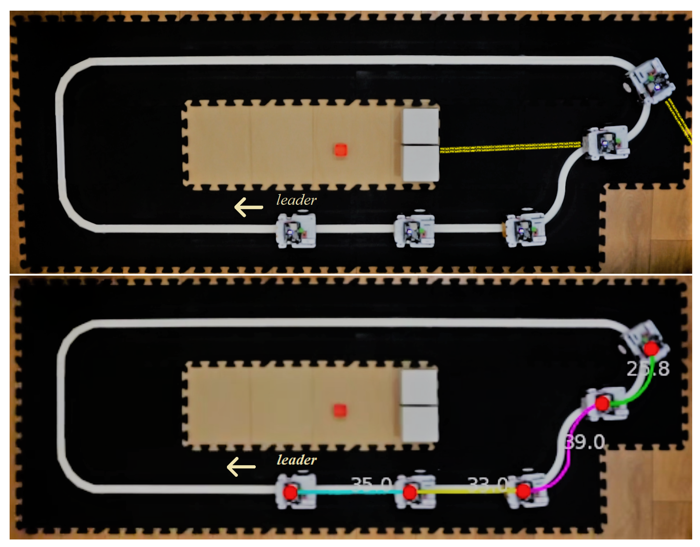
As mentioned in the previous section, the framework considers that distance measurements obtained from the ranging sensors may be unreliable. In the context of the experimental setup based on the RUPU platform, the main factor that affects the reliability of the distance sensors is the temporary loss of the line of sight when the vehicles move along a curve. Without having a vehicle in the line of sight, the measurement will be relative to the closest object in the environment. Figure 5 shows an example situation that illustrates the difficulty, where the last two agents do not have a preceding vehicle in the line of sight of its ranging sensor (shown with a yellow line). Therefore, the measured distance using the sensor, $d^m\left(t\right)$, and used by the controller, will not always be equal to the true inter-vehicle distance $d\left(t\right)$.

To evaluate the performance of the proposed control strategy, we implemented an offline algorithm to estimate an approximate value for $d\left(t\right)$ using computer-vision techniques. The outcome of the algorithm for an example scenario is depicted in the bottom picture in Figure 5, where the same scenario shown in the top part now includes estimated values for all inter-vehicle distances, emphasized with different colors. The algorithm calculates the inter-vehicle distance as the shortest path along the line between two markers in consecutive agents. Assuming that the agents are similar and the markers are positioned at the same point on each vehicle, we can then obtain the shortest distance by subtracting the length of an agent from the value delivered by the algorithm. It is important to highlight that $d\left(t\right)$ is not employed online for control purposes and only serves as a reference value to evaluate the control performance using a reliable and consistent measurement of the distance tracking error.

4. Cooperative Control Strategy

The proposed cooperative strategy to design local controllers aims to deal with the lateral and longitudinal problems in line-following platooning and also provide robustness against unreliable distance measurements generated, for instance, in curved paths. The proposed controller is based on the dynamical model of the RUPU platform; however, the underlying cooperative control technique can be adapted and employed for different models.

We maintain here the simplified notation, omitting the index i. The proposed control exploits the structure of the system model in Equation (5), considering the inter-vehicle distance as an output, and it can include in the control loop the velocity of the predecessor vehicle, which is received using wireless communication. Indeed, from Equation (9), we note that it is possible to include the matrix $M_u$ as a part of the controller and define a new input vector as

$$\begin{array}{c}\hfill \left[\begin{array}{c}{U}_d\left(s\right)\\ U_{\theta }\left(s\right)\end{array}\right]=\underset{M_u}{\underbrace{\left[\begin{array}{cc}1& 1\\ 1& -1\end{array}\right]}}U\left(s\right)=\left[\begin{array}{c}{U}_{mr}\left(s\right)+U_{ml}\left(s\right)\\ U_{mr}\left(s\right)-U_{ml}\left(s\right)\end{array}\right].\end{array}$$

(10)

This yields $V\left(s\right)=G_{11}\left(s\right)U_d\left(s\right)$, $D\left(s\right)=G_{21}\left(s\right)U_d\left(s\right)$ and $\theta \left(s\right)=G_{31}\left(s\right)U_{\theta }\left(s\right)$. Since we can only manipulate two variables ($U_d\left(s\right)$ and $U_{\theta }\left(s\right)$) we cannot control $V\left(s\right)$ and $D\left(s\right)$ independently. Indeed, when controlling the distance $D\left(s\right)$, we implicitly control $V\left(s\right)$, since $G_{11}\left(s\right)=s{G}_{21}\left(s\right)$.

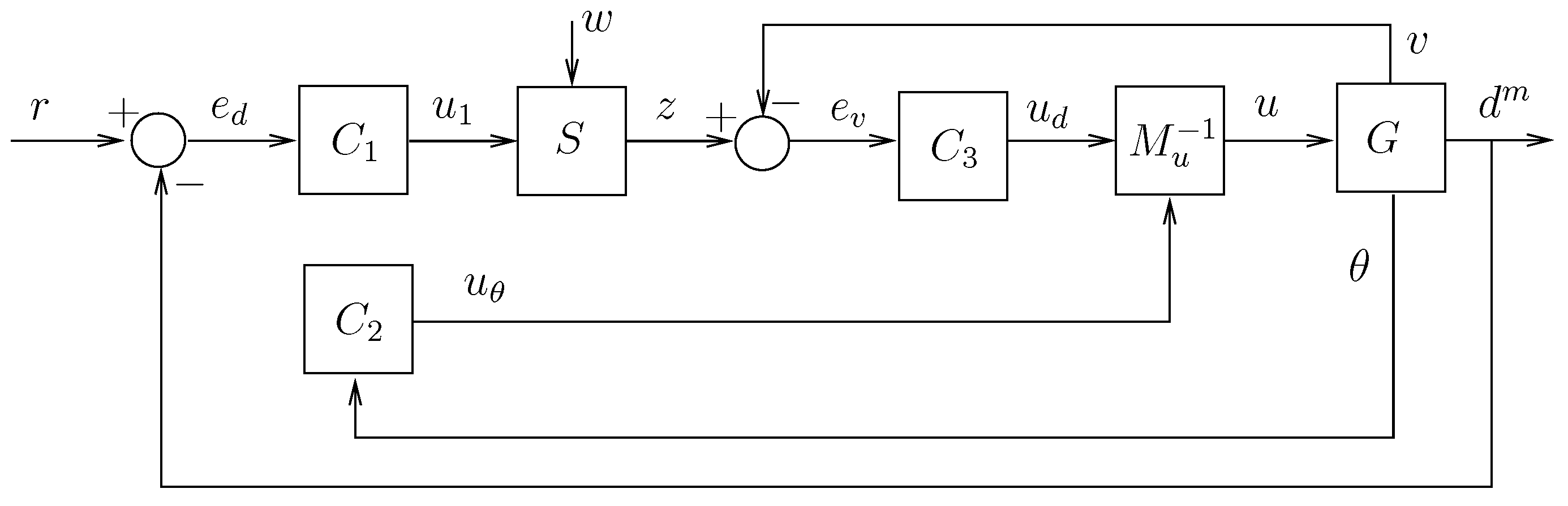
In our proposed cooperative algorithm, we exploit the communication topology to enhance the control scheme, including an inner loop to manipulate the speed using the velocity of the predecessor agent. This inner loop allows us to perform speed control in case the distance sensing is unreliable. Moreover, we should recall that the true distance $d\left(t\right)$ is assumed to be known to derive the model; however, the controller uses the distance measured by the local sensor $d^m\left(t\right)$, which may not be equal to $d\left(t\right)$. Consequently, we use the control loop depicted in Figure 6, where $C_1\left(s\right)$, $C_2\left(s\right)$, and $C_3\left(s\right)$ are SISO controllers to be designed with integral action, where $M_u^{-1}$ allows for recovering the true voltage signals given that

$$\begin{array}{cc}\hfill U_{mr}\left(s\right)& =(U_d\left(s\right)+U_{\theta }\left(s\right))/2\hfill \end{array}$$

(11)

$$\begin{array}{cc}\hfill U_{ml}\left(s\right)& =(U_d\left(s\right)-U_{\theta }\left(s\right))/2.\hfill \end{array}$$

(12)

The cooperative feature of this control technique affects the inner loop controlling the velocity. We explicitly use the information of the predecessor’s velocity as a part of a function to limit the speed reference of the agent, which is represented in Figure 6 by the block denoted by S. The inputs of S are the output of the dynamic controller $C_1\left(s\right)$, denoted by $u_1$, and the velocity of the predecessor agent, which is denoted by w and is transmitted wirelessly. The signal z is the output of S, and given by

$$\begin{array}{cc}\hfill z\left(t\right)& =\left\{\begin{array}{ccc}{S}_u\left(t\right)\hfill & \mathrm{for}& u_1\left(t\right)\ge S_u\left(t\right)\hfill \\ u_1\left(t\right),\hfill & \mathrm{for}& S_l\left(t\right)<u_1\left(t\right)<S_u\left(t\right)\hfill \\ S_l\left(t\right),\hfill & \mathrm{for}& u_1\left(t\right)\le S_l\left(t\right)\hfill \end{array}\right.\hfill \end{array}$$

(13)

where $S_u\left(t\right)$ and $S_l\left(t\right)$ are functions that depend on w and represent the upper and lower limits of $u_1$, respectively. The limiting functions are chosen to be

$$\begin{array}{cc}\hfill S_u\left(t\right)& =\alpha w\left(t\right)+ϵ,S_l\left(t\right)=\beta w\left(t\right)-ϵ,\mathrm{for}w\left(t\right)\ge 0\hfill \end{array}$$

(14)

$$\begin{array}{cc}\hfill S_u\left(t\right)& =\beta w\left(t\right)+ϵ,S_l\left(t\right)=\alpha w\left(t\right)-ϵ,\mathrm{for}w\left(t\right)<0\hfill \end{array}$$

(15)

where $\alpha \ge 1$, $0<\beta \le 1$, and $ϵ>0$, are parameters to be chosen such that $S_u\left(t\right)$ and $S_l\left(t\right)$ are close to the predecessor’s velocity. A natural choice in a practical scenario is $\alpha$ and $\beta$ being close to 1, and $ϵ$ being close to 0.

Given the control scheme, $z\left(t\right)$ can be viewed as a speed reference for the agent, which is governed by the distance tracking error and limited by the predecessor’s speed. This allows the agent to keep a velocity close to the predecessor’s, but not necessarily equal, allowing it to perform the distance tracking properly. The values of $\alpha$, $\beta$, and $ϵ$ can be adjusted to achieve a desired transient response. In steady-state, distance and velocity tracking should be equal to zero due to the integral action. Note that, for high values of $ϵ$, the saturation may not affect, and thus this case is not a cooperative case since the predecessor’s speed $w\left(t\right)$ is not playing any role.

This strategy makes the controller less vulnerable to vigorous speed changes provoked by temporary distance sensing issues such as those due to curved paths since the inner control loop and the saturation policy prioritize speed control when distance measurement is unreliable.

5. Experimental Results

This section presents the experimental results of two case studies. The first case is a non-cooperative one, without considering the saturation stage where the predecessor’s speed is important. The second one is the cooperative case, where saturation is considered.

For the experimental setup, we use the path given in Figure 5, which has straight and curved sections and a group of five agents (one leader and four followers). We label the leader with the index 0, while the remainder agents are labeled with index $i=1,2,3,4.$ Before the experiments, the agents perform an initialization routine to position themselves aligned along a straight section of the line to follow (starting with an orientation angle error around zero) and at a predefined distance from the predecessors. During the experiments, the leader receives its velocity reference remotely from an external user. The remaining vehicles follow the leader’s trajectory but aim to maintain the inter-vehicle distance constant at 25 cm, regardless of the speed changes of the leader. For precaution, we limit the speed of each agent to 30 cm/s.

For illustrative purposes, we choose the controllers to be Proportional–Integral–Derivative (PID) for $C_1$ and $C_2$, and Proportional–Integral (PI) for $C_3$. In particular, we select

$$\begin{array}{cc}\hfill C_1\left(s\right)& =-8-5.6\frac{1}{s}-1.01s,C_2\left(s\right)=-2760+6250\frac{1}{s}+304s\hfill \\ \hfill C_3\left(s\right)& =-20.3-145\frac{1}{s}.\hfill \end{array}$$

We use the same controllers $C_1$, $C_2$, and $C_3$ for both the cooperative and the non-cooperative setups. Thus, the comparison is not with this specific controller’s performance but with the effect of incorporating the cooperative-based limiting speed stage on the platoon’s behavior.

5.1. Offline-Distance Measurement Results

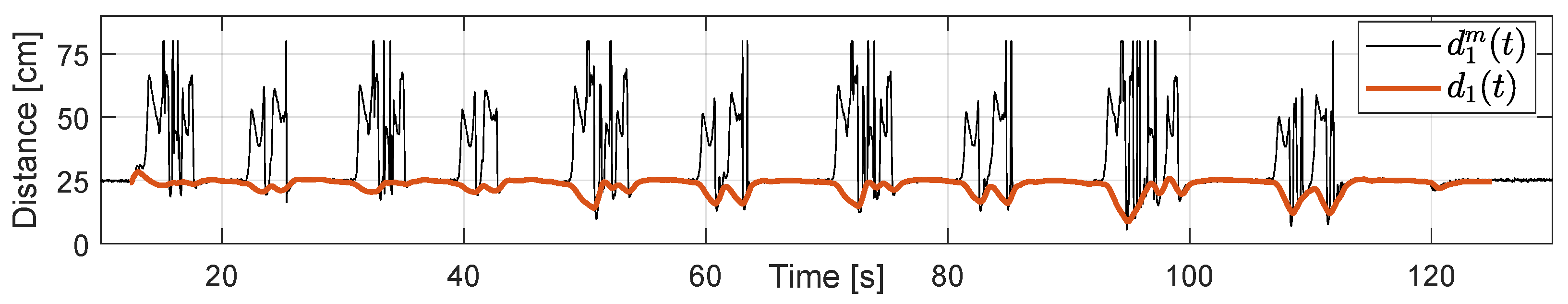
We start by showing the performance of the offline algorithm to estimate the true distances $d_i\left(t\right)$, as described in Section 3.2. As an example, Figure 7 shows the distances between the first follower and the leader, including the distance measured with the ranging sensors $d_1^m\left(t\right)$ and the estimated true distance $d_1\left(t\right)$ obtained from the offline algorithm based on computer vision techniques. The reference inter-vehicle distance is 25 cm. In the periods where $d_1^m\left(t\right)$ is close to 25 cm, the vehicles are moving along a straight section of the path; however, during curved sections, the measured distance deviates significantly from the target due to the temporal loss of the line of sight of the sensor, making the measurements unreliable and not representative of the actual inter-vehicle distance. On the other hand, the estimated distance $d_1\left(t\right)$ from the offline algorithm matches $d_1^m\left(t\right)$ during straight path periods but also provides reliable measurements during curves. Similar behavior is verified for different agents, speeds, and distance references.

For the distance tracking analysis in the following sections, we use $d_i\left(t\right)$ instead of $d_i^m\left(t\right)$. However, we recall that $d_i\left(t\right)$ is obtained offline for validation purposes and is not used for the control tasks. The implemented controllers use $d_i^m\left(t\right)$ to perform the experiments.

5.2. Experimental Results for the Non-Cooperative Case

In this case, we consider that the saturation block in the control scheme in Figure 6 is not present, and thus, the predecessor’s speed does not play any role. The control is implemented based only on the measured distance $d_i\left(t\right)$. The dynamic behavior of the platoon is summarized in Figure 8, Figure 9, Figure 10 and Figure 11. A video of the experiment showing the operational conditions and the platoon behavior is available here: https://youtu.be/JvotmTYlXOY (accessed on 16 January 2023).

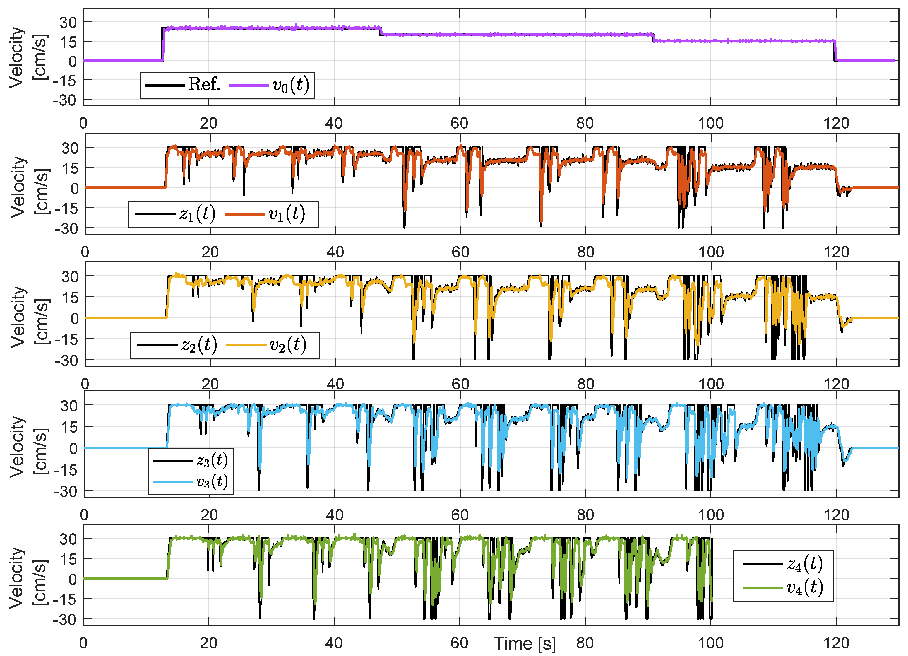
The plots in Figure 8 show the velocity of each agent. The leader receives an external stair-type velocity reference, which is tracked without problems. The rest of the agents do not receive an external reference but generate an internal one through distance control. We can see that the agent velocities $v_i\left(t\right)$ follow the corresponding references $z_i\left(t\right)$, although with some transient errors. The main observation in this plot is that the velocity references $z_i\left(t\right)$ are erratic as a consequence of tracking the unreliable distance $d_i^m$. During curves, the measured distances $d_i^m\left(t\right)$ are higher than the real value (see Figure 7), and thus the controller increases the speed vigorously to reach the desired inter-vehicle distance. At some point, the agent leaves the curve and enters a straight section, and the distance sensor suddenly detects the predecessor, which is closer than expected, and therefore, the follower moves in the opposite direction. Actually, in this experiment, some $z_i\left(t\right)$ change abruptly from 30 cm/s to $-30$ cm/s, provoking an oscillatory behavior. Indeed, the last agent collides with its predecessors at approximately 100 s and moves out from the path. The experiment finishes a few seconds later. For higher speeds of the leader, agents are less sensitive to unreliable distance measures since the periods on curved sections are shorter, but at a low leader speed, the influence of the curves is aggravated.

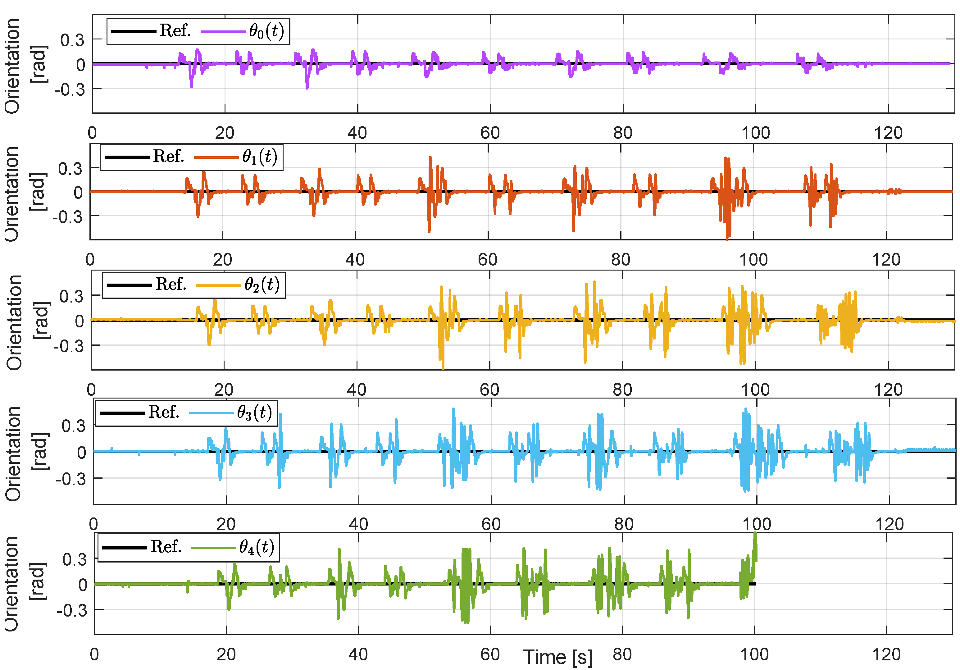
The distance tracking is shown in Figure 9 for each agent, except for the leader. Clearly, agents can be considerably closer than expected during curves due to the behavior mentioned above, yielding the worst performance for the last agent, which ultimately collides with its predecessor. On the other hand, errors in the orientation measurement are also associated with curved paths. In this case, errors are not related to a sensing issue but rather an intrinsic disturbance due to the alignment of the infrared sensors that detect the line in the path. This can be aggravated by erratic behavior due to improper distance tracking. This behavior is illustrated in Figure 10, where the orientation angles for each vehicle are plotted, which also correspond to the orientation error since ${\theta }_i=e_{{\theta }_i}$ (see Equation (1)). The leader presents an acceptable performance in terms of orientation with respect to the line, achieving zero error during straight sections of the path and maintaining low transient deviation angles during curves; however, such a performance level is not reached by the followers, whose orientation errors are considerably higher when moving along curves. We also note that such angles are higher at lower velocities and, actually, near $t=100$, we observe peak values around $\pm 0.6\left[\mathrm{rad}\right]\approx \pm {34}^{\circ }$. Figure 11 presents a zoomed-in version of a region of interest for all plots in Figure 10, which also include the corresponding graphs of the velocity and distance tracking errors. The magnification of the plots is on a time window where a change of speed from 25 cm/s to 20 cm/s is performed by the leader. We can see that the errors increase as the disturbance propagates from the first agent to the last one, suggesting that the controller performs in a string-unstable fashion [37]. This could be corrected by changing the controller parameters; however, string stabilization is not within the scope of this paper.

5.3. Experimental Results for the Cooperative Case

In this case, we include the saturation stage of the proposed control scheme with $ϵ=1$, $\alpha =1.1$, and $\beta =0.9$, for each agent. The velocity of the predecessor is transmitted wirelessly. The rest of the control scheme, including the controller $C_1$, $C_2$, and $C_3$, is the same as in the previous experiment. By incorporating the saturation stage, each follower uses the internal signal $z_i$ as a velocity reference, which now strongly depends on the estimated predecessor velocity. Implementing this control scheme requires inter-agent communication so that each vehicle can communicate its local velocity to its follower. The experimental results are given in Figure 12, Figure 13, Figure 14 and Figure 15. The video of the reported experiment is available here: https://youtu.be/uK39YJ0bv1M (accessed on 16 January 2023).

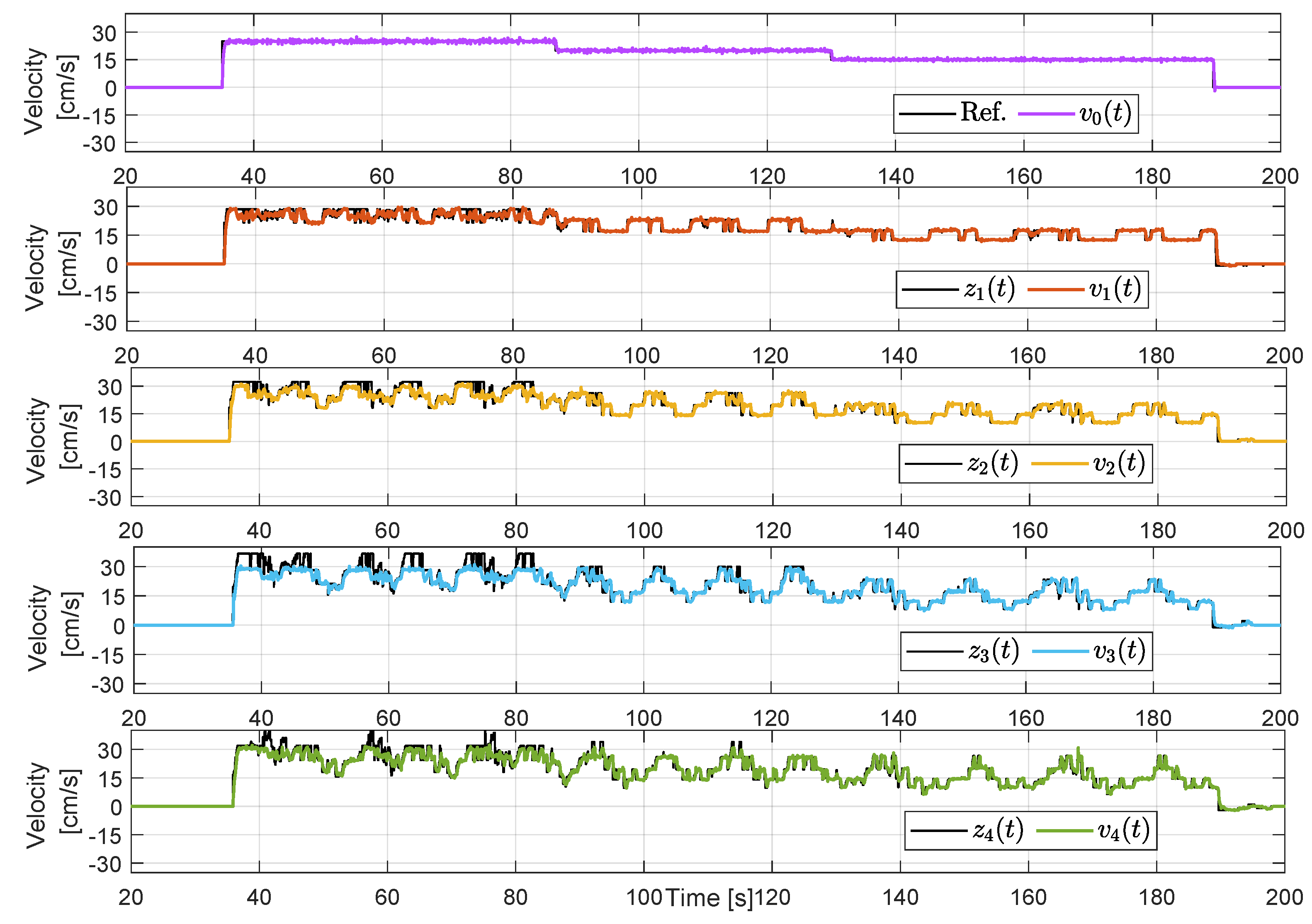
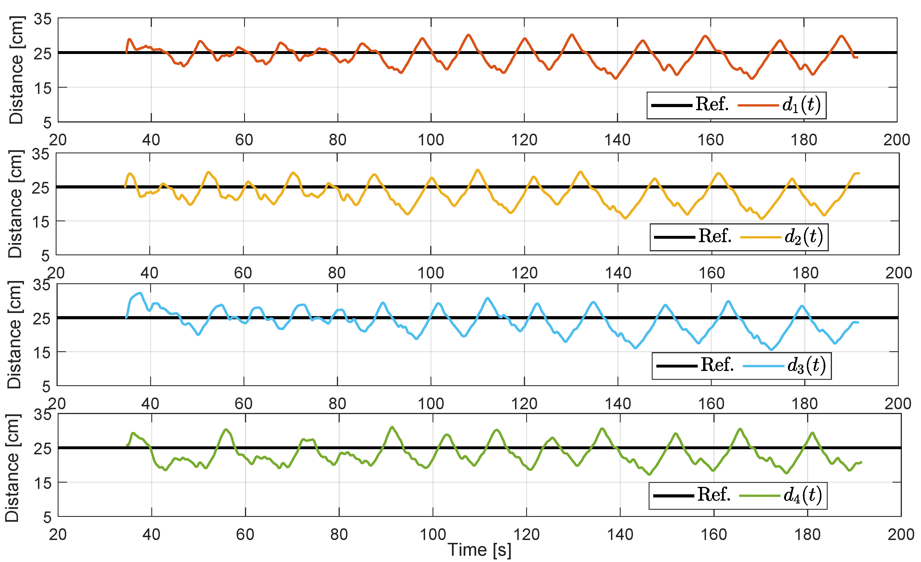
The velocity tracking results are presented in Figure 12. In this case, the experiment is more extended since, unlike the non-cooperative case, it is not aborted due to agent collisions. In this case, the leader and the followers adequately follow their corresponding velocity reference. A key difference, in this case, is that the internal references $z_i$ are now less vigorous due to the effect of the saturation stage. We recall that the measured distances $d_i^m\left(t\right)$ are still erratic as the ones in Figure 7; however, the effect provoked by such unreliable measurement is considerably reduced by the limits imposed by the predecessors’ velocities. In this case, none of the agents have negative velocities; thus, the group of agents always moves forward. Figure 13 shows the distance tracking results. Distance tracking is also affected by curves, and we can note that a close-to-zero tracking error is not achieved most of the time; however, the cooperative case performs better than the non-cooperative case, where agents could be too close. Although agents do not behave abruptly as in the previous case, settling times may be slower due to saturation, which explains why tracking errors are not zero most of the time during straight sections of the path. Nevertheless, the platoon movement is much more fluent and avoids collisions see https://youtu.be/uK39YJ0bv1M (accessed on 16 January 2023).

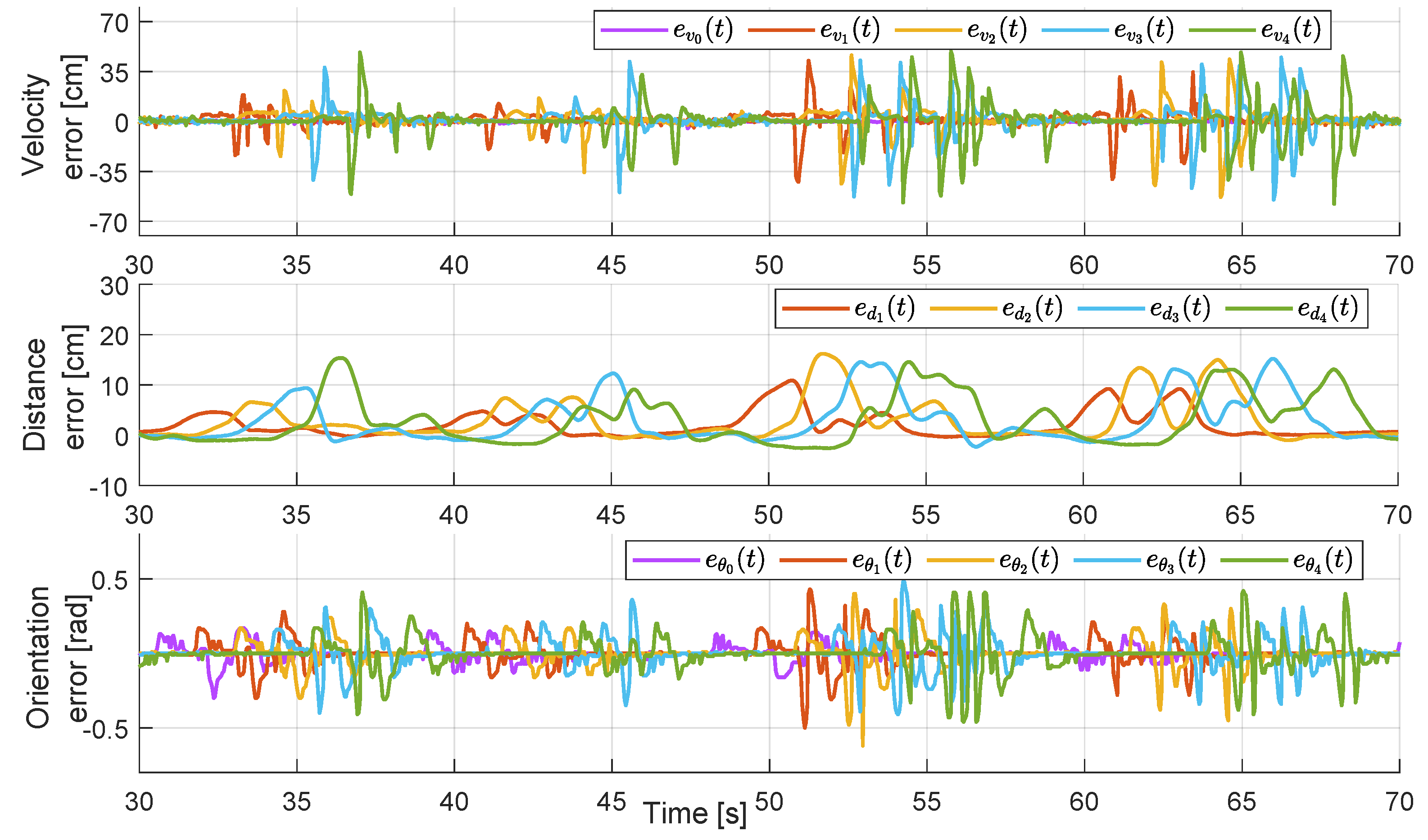
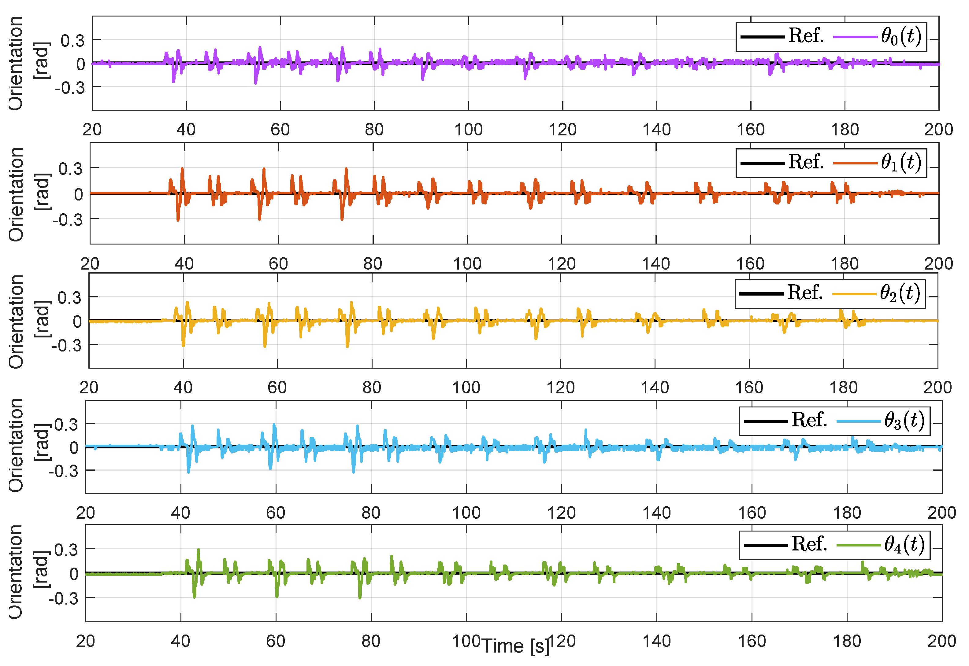
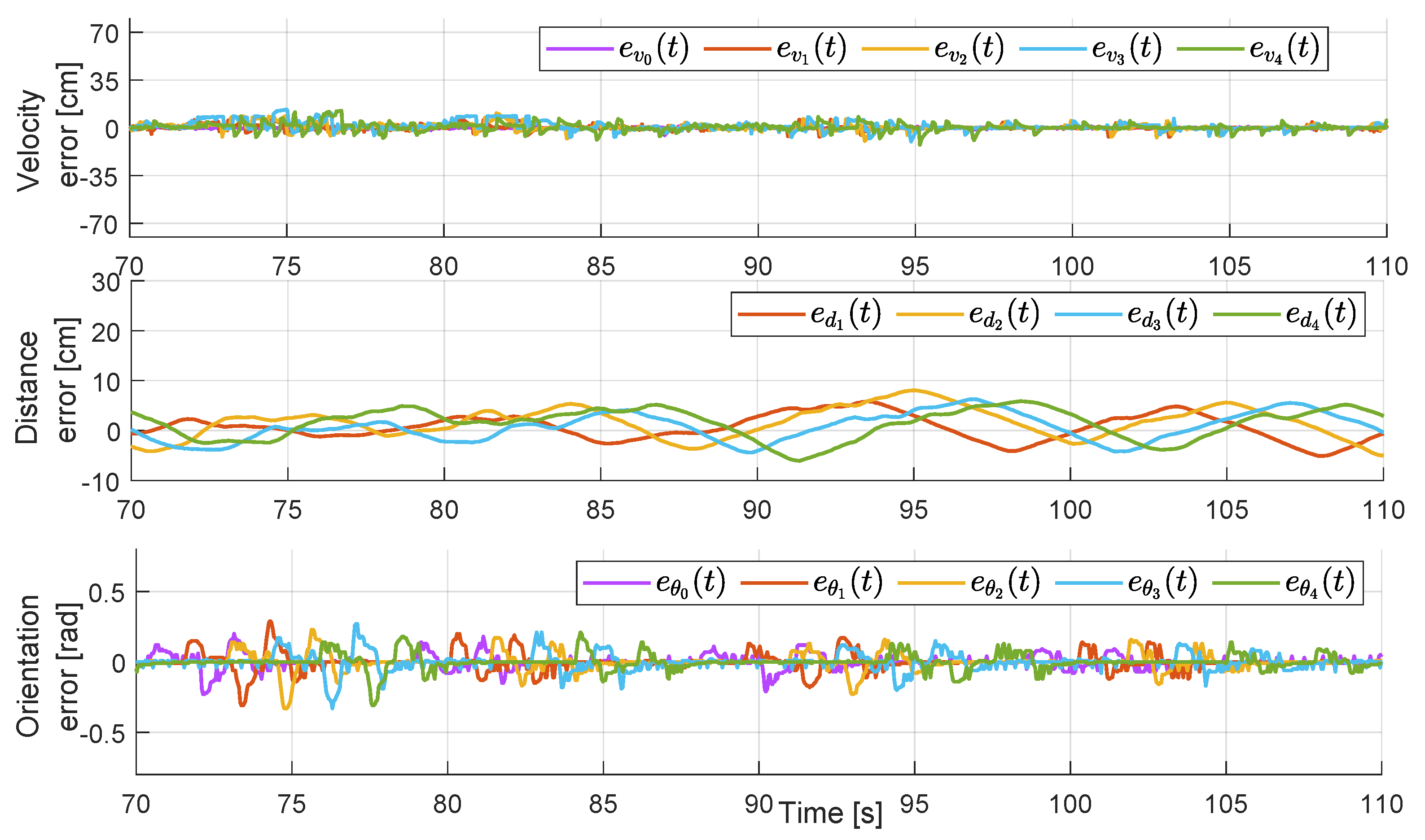
Figure 14 summarizes results related to the orientation control (angle tracking). Clearly, the controller follows the reference with transient errors during the curves, but the performance is considerably better than in the non-cooperative case. Indeed, the control strategy effectively maintains the angle around zero with oscillations in the range $\pm 0.3\left[\mathrm{rad}\right]\approx \pm {17}^{\circ }$ at the beginning of the experiment, which decreases as the velocity decreases. This behavior is the opposite of the non-cooperative case in Figure 10. Figure 15 shows a more detailed view of the transient behavior during the time window that encloses the change in the leader’s velocity reference from 25 cm/s to 20 cm/s. The plots in Figure 15 can be directly compared with the ones in Figure 11, where we can observe that velocity, distance, and orientation errors are considerably lower in the cooperative case compared to the non-cooperative case.

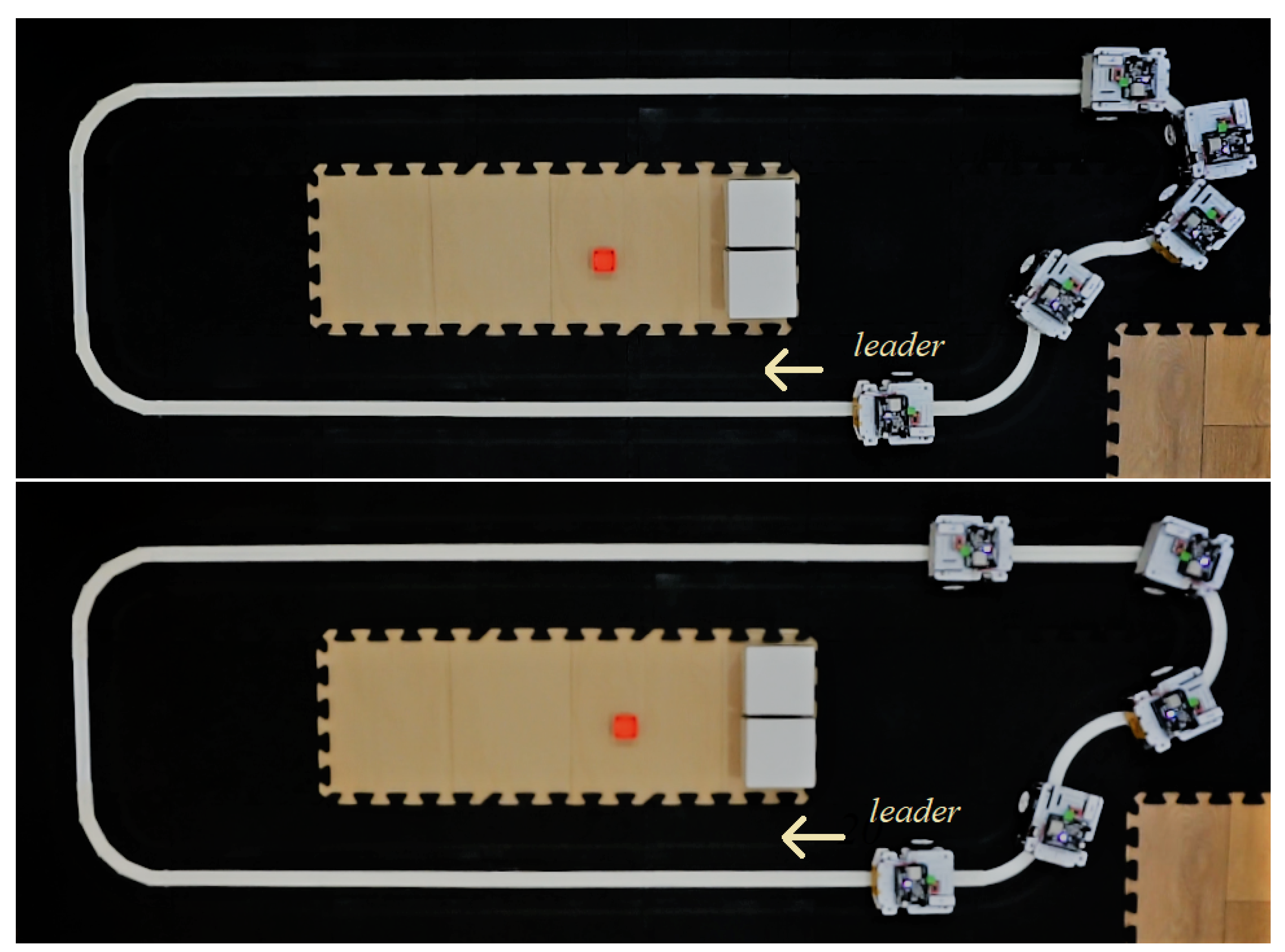
We can also visually inspect the global performance of the platoon in the provided videos, where we observe a notable improvement in the cooperative scheme. Figure 16 shows an example of an equivalent relevant scenario considering both non-cooperative and cooperative control schemes. Specifically, we considered the leader to be the independent and common subject and took a frame when the leader leaves the first curve after changing its velocity from 20 cm/s to 15 cm/s. The platoon performs poorly in the non-cooperative case, even with collisions in the last vehicles. In an equivalent scenario, the cooperative case shows better tracking of the inter-vehicle distance for all vehicles.

6. Conclusions

We presented a cooperative control scheme to deal with unreliable measurements of the inter-vehicle distance in line-following platooning problems. In this control strategy, the velocity of a predecessor is used to limit the speed of the vehicles, avoiding vigorous reactions due to the temporary erroneous sensing derived from the limited line-of-sight of ranging sensors. We used the RUPU experimental platform to test the proposed control algorithm and compare it to a non-cooperative strategy. The RUPU platform is a low-cost platform specifically designed for testing different cooperative platooning schemes and related problems of relevance. The experimental results illustrate the proposed control algorithm’s effectiveness in dealing with unreliable distance sensing and also showcase the capabilities of the experimental platform.

Future work includes the analytical study for string stabilizing control design in the proposed setup, the exploration of new control architectures in line-following platooning, and the usage of new cooperative policies to deal with practical issues that may arise in large platoon formations, such as sensing and communication issues.

References

- Dey, K.C.; Yan, L.; Wang, X.; Wang, Y.; Shen, H.; Chowdhury, M.; Yu, L.; Qiu, C.; Soundararaj, V. A review of communication, driver characteristics, and controls aspects of cooperative adaptive cruise control (CACC). IEEE Trans. Intell. Transp. Syst. 2015, 17, 491–509. [Google Scholar] [CrossRef]
- Wang, Z.; Wu, G.; Barth, M.J. A Review on Cooperative Adaptive Cruise Control (CACC) Systems: Architectures, Controls, and Applications. In Proceedings of the 2018 21st International Conference on Intelligent Transportation Systems (ITSC), Maui, HI, USA, 4–7 November 2018; pp. 2884–2891. [Google Scholar] [CrossRef]
- Wang, C.; Gong, S.; Zhou, A.; Li, T.; Peeta, S. Cooperative adaptive cruise control for connected autonomous vehicles by factoring communication-related constraints. Transp. Res. Part Emerg. Technol. 2020, 113, 124–145. [Google Scholar] [CrossRef]
- Li, S.E.; Zheng, Y.; Li, K.; Wu, Y.; Hedrick, J.K.; Gao, F.; Zhang, H. Dynamical Modeling and Distributed Control of Connected and Automated Vehicles: Challenges and Opportunities. IEEE Intell. Transp. Syst. Mag. 2017, 9, 46–58. [Google Scholar] [CrossRef]
- Guerrero-Ibáñez, J.; Zeadally, S.; Contreras-Castillo, J. Sensor technologies for intelligent transportation systems. Sensors 2018, 18, 1212. [Google Scholar] [CrossRef] [PubMed]
- Turri, V.; Besselink, B.; Johansson, K.H. Cooperative look-ahead control for fuel-efficient and safe heavy-duty vehicle platooning. IEEE Trans. Control Syst. Technol. 2016, 25, 12–28. [Google Scholar]
- Thormann, S.; Schirrer, A.; Jakubek, S. Safe and efficient cooperative platooning. IEEE Trans. Intell. Transp. Syst. 2020, 2, 1368–1380. [Google Scholar] [CrossRef]
- Jia, D.; Lu, K.; Wang, J.; Zhang, X.; Shen, X. A survey on platoon-based vehicular cyber-physical systems. IEEE Commun. Surv. Tutor. 2015, 18, 263–284. [Google Scholar] [CrossRef]
- Bergenhem, C.; Shladover, S.; Coelingh, E.; Englund, C.; Tsugawa, S. Overview of platooning systems. In Proceedings of the 19th ITS World Congress, Vienna, Austria, 22–26 October 2012. [Google Scholar]
- Jiang, J.; Astolfi, A. Lateral Control of an Autonomous Vehicle. IEEE Trans. Intell. Veh. 2018, 3, 228–237. [Google Scholar] [CrossRef]
- Swaroop, D.; Hedrick, J.K.; Choi, S.B. Direct adaptive longitudinal control of vehicle platoons. IEEE Trans. Veh. Technol. 2001, 50, 150–161. [Google Scholar]
- Dang, D.; Gao, F.; Hu, Q. Motion planning for autonomous vehicles considering longitudinal and lateral dynamics coupling. Appl. Sci. 2020, 10, 3180. [Google Scholar] [CrossRef]
- Chebly, A.; Talj, R.; Charara, A. Coupled longitudinal/lateral controllers for autonomous vehicles navigation, with experimental validation. Control Eng. Pract. 2019, 88, 79–96. [Google Scholar] [CrossRef]
- Zhou, H.; Jia, F.; Jing, H.; Liu, Z.; Güvenç, L. Coordinated longitudinal and lateral motion control for four wheel independent motor-drive electric vehicle. IEEE Trans. Veh. Technol. 2018, 67, 3782–3790. [Google Scholar] [CrossRef]
- Latrech, C.; Chaibet, A.; Boukhnifer, M.; Glaser, S. Integrated Longitudinal and Lateral Networked Control System Design for Vehicle Platooning. Sensors 2018, 18, 3085. [Google Scholar] [CrossRef]
- Bayuwindra, A.; Ploeg, J.; Lefeber, E.; Nijmeijer, H. Combined Longitudinal and Lateral Control of Car-Like Vehicle Platooning With Extended Look-Ahead. IEEE Trans. Control Syst. Technol. 2020, 28, 790–803. [Google Scholar] [CrossRef]
- Yu, L.; Bai, Y.; Kuang, Z.; Liu, C.; Jiao, H. Intelligent Bus Platoon Lateral and Longitudinal Control Method Based on Finite-Time Sliding Mode. Sensors 2022, 22, 3139. [Google Scholar] [CrossRef]
- Badue, C.; Guidolini, R.; Carneiro, R.V.; Azevedo, P.; Cardoso, V.B.; Forechi, A.; Jesus, L.; Berriel, R.; Paixão, T.M.; Mutz, F.; et al. Self-driving cars: A survey. Expert Syst. Appl. 2021, 165, 113816. [Google Scholar] [CrossRef]
- Bautista-Camino, P.; Barranco-Gutiérrez, A.I.; Cervantes, I.; Rodríguez-Licea, M.; Prado-Olivarez, J.; Pérez-Pinal, F.J. Local Path Planning for Autonomous Vehicles Based on the Natural Behavior of the Biological Action-Perception Motion. Energies 2022, 15, 1769. [Google Scholar] [CrossRef]
- Claussmann, L.; Revilloud, M.; Gruyer, D.; Glaser, S. A Review of Motion Planning for Highway Autonomous Driving. IEEE Trans. Intell. Transp. Syst. 2020, 21, 1826–1848. [Google Scholar] [CrossRef]
- Gupta, A.; Anpalagan, A.; Guan, L.; Khwaja, A.S. Deep learning for object detection and scene perception in self-driving cars: Survey, challenges, and open issues. Array 2021, 10, 100057. [Google Scholar] [CrossRef]
- Ingle, S.; Phute, M. Tesla autopilot: Semi autonomous driving, an uptick for future autonomy. Int. Res. J. Eng. Technol. 2016, 3, 369–372. [Google Scholar]
- The New York Times. What Riding in a Self-Driving Tesla Tells Us about the Future of Autonomy. 2022. Available online: https://www.nytimes.com/interactive/2022/11/14/technology/tesla-self-driving-flaws.html (accessed on 16 January 2023).
- Rosique, F.; Navarro, P.J.; Fernández, C.; Padilla, A. A Systematic Review of Perception System and Simulators for Autonomous Vehicles Research. Sensors 2019, 19, 648. [Google Scholar] [CrossRef] [PubMed]
- Sybis, M.; Rodziewicz, M.; Wesołowski, K. Influence of Sensor Inaccuracies and Acceleration Limits on IEEE 802.11p-Based CACC Controlled Platoons. In Proceedings of the 2020 IEEE 91st Vehicular Technology Conference (VTC2020-Spring), Antwerp, Belgium, 25–28 May 2020; pp. 1–6. [Google Scholar]
- Lengyel, H.; Tettamanti, T.; Szalay, Z. Conflicts of Automated Driving With Conventional Traffic Infrastructure. IEEE Access 2020, 8, 163280–163297. [Google Scholar] [CrossRef]
- Yin, S.; Yang, C.; Kawsar, I.; Du, H.; Pan, Y. Longitudinal Predictive Control for Vehicle-Following Collision Avoidance in Autonomous Driving Considering Distance and Acceleration Compensation. Sensors 2022, 22, 7395. [Google Scholar] [CrossRef] [PubMed]
- Stüdli, S.; Seron, M.; Middleton, R. From vehicular platoons to general networked systems: String stability and related concepts. Annu. Rev. Control 2017, 44, 157–172. [Google Scholar] [CrossRef]
- Feng, S.; Zhang, Y.; Li, S.E.; Cao, Z.; Liu, H.X.; Li, L. String stability for vehicular platoon control: Definitions and analysis methods. Annu. Rev. Control 2019, 47, 81–97. [Google Scholar] [CrossRef]
- Gordon, M.A.; Vargas, F.J.; Peters, A.A. Comparison of Simple Strategies for Vehicular Platooning with Lossy Communication. IEEE Access 2021, 9, 103996–104010. [Google Scholar] [CrossRef]
- Gordon, M.A.; Vargas, F.J.; Peters, A.A. Mean square stability conditions for platoons with lossy inter-vehicle communication channels. Automatica 2023, 147, 110710. [Google Scholar] [CrossRef]
- Ensemble. Available online: https://platooningensemble.eu (accessed on 16 January 2023).
- Widyotriatmo, A.; Siregar, P.I.; Nazaruddin, Y.Y. Line following control of an autonomous truck-trailer. In Proceedings of the 2017 International Conference on Robotics, Biomimetics, and Intelligent Computational Systems (Robionetics), Bali, Indonesia, 23–25 August 2017; pp. 24–28. [Google Scholar]
- Sezgin, A.; Çetin, Ö. Design and Implementation of Adaptive Fuzzy PD Line Following Robot. In Intelligent and Fuzzy Techniques in Big Data Analytics and Decision Making, Proceedings of the INFUS 2019 Conference, Istanbul, Turkey, 23–25 July 2019; Springer: Cham, Switzerland, 2019; pp. 106–114. [Google Scholar]
- Albertos, P.; Sala, A. Multivariable Control Systems: An Engineering Approach; Springer Science & Business Media: Berlin/Heidelberg, Germany, 2006. [Google Scholar]
- Wu, L.; Lu, Z.; Guo, G. Analysis, synthesis and experiments of networked platoons with communication constraints. Promet Traffic Traffico 2017, 29, 35–44. [Google Scholar] [CrossRef]
- Seiler, P.; Pant, A.; Hedrick, K. Disturbance propagation in vehicle strings. IEEE Trans. Autom. Control 2004, 49, 1835–1842. [Google Scholar] [CrossRef]
- Siwek, M.; Panasiuk, J.; Baranowski, L.; Kaczmarek, W.; Prusaczyk, P.; Borys, S. Identification of Differential Drive Robot Dynamic Model Parameters. Materials 2023, 16, 683. [Google Scholar] [CrossRef] [PubMed]
Figure 1.
Line-following control: (a) lateral problem (b) longitudinal problem.
Figure 2.
General feedback control loop of each vehicle.
Figure 3.
Overview of the RUPU experimental platform.
Figure 4.
Top and bottom views for a single assembled agent.
Figure 5.
Top: Unreliable measurement of the distance sensor, . Bottom: offline estimation of the true distance along the path.
Figure 6.
Cooperative control scheme with speed saturation.
Figure 7.
Offline video-based distance measurement performance.
Figure 8.
Velocity tracking using the non-cooperative strategy.
Figure 9.
Distance tracking using the non-cooperative strategy.
Figure 10.
Angle tracking using the non-cooperative strategy.
Figure 11.
Errors in a time window of the experiment using the non-cooperative strategy.
Figure 12.
Velocity tracking using the cooperative strategy.
Figure 13.
Distance tracking using the cooperative strategy.
Figure 14.
Angle tracking using the cooperative strategy.
Figure 15.
Errors in a time window of the experiment with the cooperative strategy.
Figure 16.
Visual comparison of the performance with the non-cooperative case (top) and the cooperative case (bottom).
Disclaimer/Publisher’s Note: The statements, opinions and data contained in all publications are solely those of the individual author(s) and contributor(s) and not of MDPI and/or the editor(s). MDPI and/or the editor(s) disclaim responsibility for any injury to people or property resulting from any ideas, methods, instructions or products referred to in the content. |
© 2023 by the authors. Licensee MDPI, Basel, Switzerland. This article is an open access article distributed under the terms and conditions of the Creative Commons Attribution (CC BY) license (https://creativecommons.org/licenses/by/4.0/).
Share and Cite
MDPI and ACS Style
Escobar, C.; Vargas, F.J.; Peters, A.A.; Carvajal, G. A Cooperative Control Algorithm for Line and Predecessor Following Platoons Subject to Unreliable Distance Measurements. Mathematics 2023, 11, 801. https://doi.org/10.3390/math11040801
AMA Style
Escobar C, Vargas FJ, Peters AA, Carvajal G. A Cooperative Control Algorithm for Line and Predecessor Following Platoons Subject to Unreliable Distance Measurements. Mathematics. 2023; 11(4):801. https://doi.org/10.3390/math11040801
Chicago/Turabian StyleEscobar, Carlos, Francisco J. Vargas, Andrés A. Peters, and Gonzalo Carvajal. 2023. "A Cooperative Control Algorithm for Line and Predecessor Following Platoons Subject to Unreliable Distance Measurements" Mathematics 11, no. 4: 801. https://doi.org/10.3390/math11040801
Note that from the first issue of 2016, this journal uses article numbers instead of page numbers. See further details here.