A Novel Constraint Programming Decomposition Approach for the Total Flow Time Fixed Group Shop Scheduling Problem

Abstract

This work addresses a particular case of the group shop scheduling problem (GSSP) which will be denoted as the fixed group shop scheduling problem (FGSSP). In a FGSSP, job operations are divided into stages and each stage has a set of machines associated to it which are not shared with the other stages. All jobs go through all the stages in a specific order, where the operations of the job at each stage need to be finished before the job advances to the following stage, but operations within a stage can be performed in any order. This setting is common in companies such as leaf spring manufacturers and other automotive companies. To solve the problem, we propose a novel heuristic procedure that combines a decomposition approach with a constraint programming (CP) solver and a restart mechanism both to avoid local optima and to diversify the search. The performance of our approach was tested on instances derived from other scheduling problems that the FGSSP subsumes, considering both the cases with and without anticipatory sequence-dependent setup times. The results of the proposed algorithm are compared with off-the-shelf CP and mixed integer linear programming (MILP) methods as well as with the lower bounds derived from the study of the problem. The experiments show that the proposed heuristic algorithm outperforms the other methods, specially on large-size instances with improvements of over 10% on average.

1. Introduction

In the academic world, traditional scheduling problems such as the flow shop scheduling problem, FSSP, the job shop scheduling problem, JSSP, or the open shop scheduling problem (OSSP) have been widely studied (see [1] for a general reference on scheduling problems). However, these scheduling problems may not cover all the requirements for specific manufacturing settings [2]. In this context, the group shop scheduling problem (GSSP) emerges as a generalized shop scheduling problem that includes, among others, the OSSP and the JSSP as special cases [3]. Due to its characteristics, the GSSP is a more flexible model with which address the requirements of multiple challenging real-life scheduling problems often found in the manufacturing industry.

In this paper, we consider a particular case of a GSSP that we denote as fixed group shop scheduling problem (FGSSP) [4]. In a fixed group shop environment, the operations of each job have been divided into stages, and the operations corresponding to each stage share the same set of machines. All jobs must proceed through each stage and perform the associated operations in the stage before proceeding to the next stage. Therefore, the FGSSP generalizes both OSSP and FSSP, and contains common features from many industrial environments in which manufacturing is organized in multiple sequential OSSP stages. By contrast, the classical GSSP formulation contains the OSSP and the JSSP as special cases, as each job may have a different route through the stages.

An example of a FGSSP can be found in mechanical workshops where routine car maintenance operations are performed. The number of operations for each job (car) and their processing times depend on different factors as the odometer count or the time between maintenances. For each car the set of maintenance operations can be divided into stages and the tasks to be performed on each stage must be completed before proceeding to the next stage (i.e., change the air filter, change the motor oil, etc.) with an ordering of stages predefined by the layout of the workshop, but there is no specific order in which operations within a single stage are to be performed (i.e., they have no relationship between them). Additionally, some setup operations may be required between jobs performed in a single machine, and thus sequence-dependent setup times are to be expected.

Another example of the FGSSP can be found in the manufacturing process of leaf springs. Each leaf requires several punching and forming operations that can be performed in any order. Once all these operations have been performed, the leaf is transferred to the heat treatment, sandblasting, painting, and assembly workstations. In the computational experiments section, see Section 6, we present a case study taken from a Colombian automotive company that falls within this specific example of application.

As in any other scheduling problems, multiple objective functions may be considered. In this work, we consider minimizing the total flow time.

To the best of our knowledge, the FGSSP has not been studied before even if the model has practical applications. Due to its computational complexity, it subsumes several well-known hard-to-solve problems. This work presents a novel ad hoc heuristic approach to solving the FGSSP with and without anticipatory sequence-dependent setup times under the total flow time minimization objective. According to the three-field notation proposed in [5], these problems can be denoted as the $FGSS{P}_s\mid S_{jik}\mid {\sum }_j{C}_j$ and the $FGSS{P}_s\mid \mid {\sum }_j{C}_j$, respectively.

The proposed heuristic relies on decomposing the problem into smaller subproblems and solving each subproblem through constraint programming (CP) [6] for a fixed amount of time. The heuristic can be seen as a hybrid metaheuristic [7] or a matheuristic [8] as it combines two optimization solution methods (i.e., a heuristic and an exact method approach). To test the performance of the decomposition approach, we performed extensive computational experiments with small, medium and large instances. We report the results of a computational study in which we compare our approach with off-the-shelf state-of-the-art CP and mixed integer linear programming (MILP) approaches. The results show the validity of our decomposition approach over a traditional method providing significant improvements over commercial solvers, specially for large instances.

The remainder of the paper is organized as follows. Section 2 reviews the literature on problems with similar characterstics to the FGSSP. Section 3 introduces the FGSSP, provides a problem definition, and gives an illustrative example of it. Section 4 puts forward a MILP and a CP formulation for the problem, and provides some lower bounds on the optimal objective value. Section 5 describes the decomposition-based procedure used to solving the problem, including the generation of initial solutions, the local search phase, and a shaking procedure designed to escape from local optima. Section 6 provides the results of the computational experiments conducted to test the method, as well as an industrial case study. Finally, Section 7 concludes and provides some possible research lines.

2. Literature Review

Scheduling corresponds to the allocation of scarce resources (i.e., machines) to perform tasks (i.e., jobs) over time [1]. Due to its generality and broad use, scheduling has become an important area within the operations research (OR) and operations management (OM) communities that focus their contributions on the development of decision-making methods to optimize one or multiple goals.

Among the scheduling problems, we focus our attention on a family known as “shop” problems. Among the different classifications of “shop” problems we are interested in a classification based on (i) their routes, that is, the path that the jobs must follow on the machines and, (ii) the sequence of operations that must be processed in each machine. The most common models in the literature consider that jobs follow a unique route (the FSSP), each job has its own route (the JSSP), or arbitrary routes (the OSSP)—but other cases exist. For these cases more elaborate models are needed to cope with different scheduling conditions.

An early example of these models can be found in [9]. In [9] the authors propose a hybrid model denoted as the mixed shop scheduling problem (MSSP) problem in which some jobs have their own predefined routes (i.e., as in a JSSP) and some jobs do not (i.e., as in an OSSP). Another example of alternative route schemes is the group shop scheduling problem (GSSP), also known as the stage shop problem [10]. The GSSP generalizes the MSSP and considers a set of distinct machines that perform operations on the jobs. Each stage must perform a subset of operations associated to the jobs and can perform these operations in any order within the stage, but the stages to be must be processed in a predetermined order. Note that the MSSP is a special case of GSSP, in which each stage has one operation or there is only one stage that contains all operations [11].

We now proceed to review the literature on the GSSP, as well as some works that make use of CP approaches within the scheduling literature.

The literature of the GSSP is abundant and mainly focuses on the makespan minimization objective [3,12,13,14,15,16,17,18,19]; other optimization objectives for the GSSP have been less studied. An example of other objectives can be found in [20], where the authors propose an application of a chance-constrained version of the GSSP with a total weighted completion time objective.

Sequence-dependent setup times, as well as transportation times have also been studied within the GSSP literature, [13]. In [21] the authors considered the use of a robot to transport material through the multiple processing stages in a GSSP environment.

Additionally, other publications have addressed stochastic and/or fuzzy extensions for the GSSP [12,13,20,22,23].

Regarding solution procedures, most of the literature focuses on metaheuristic approaches. Among them, genetic algorithms [13,18], Tabu Search [11,16,18,24], artificial bee colonies [17], iterated local search [24], Simulated Annealing [24], evolutionary algorithms [24], multi-start multi-level evolutionary local search [15] and ant colony optimization [3,24] are the most common. According to [24] the Tabu search showed the best results among the compared methods (an ant colony optimization, an evolutionary algorithm, an iterated local search, and a simulated annealing approach).

Exact methods, such as constraint programming (CP), have also been used to solve scheduling problems but, to the best of our knowledge, they have not been used to address the GSSP or similar problems. We review the works on exact methods for shop scheduling problems that are relevant to the method proposed in this work.

In [25] the authors proposed a CP approach to solve the JSSP, and in [26] the authors propose a CP approach to solve the OSSP. The approach proposed in [26] uses a new upper bound heuristic combined with constraint propagation and a branching technique to solve the problem. In [27] the authors proposed MILP and CP models to solve the online printing shop scheduling problem (OPSSP). The OPSSP can be seen as a JSSP where there are multiple units of some of the machines (hence, leading to a degree of flexibility within the sequence of operations for each job). The numerical experiments in [26] show that the CP method outperforms the MILP approach by a large extent. In [28], the authors used a CP model as their benchmark to compare the performance of a variable neighborhood search (VNS) for the OSSP with travel/setup times. Their VNS makes use of a probabilistic learning mechanism to self-tune a parameter that balance the generation of active or non-delay solutions. More recently, in [29] the authors proposed four CP formulations to tackle four complex flexible shop scheduling problems (i.e., the no-wait hybrid flow shop scheduling problem, the hybrid flow shop scheduling problem with sequence-dependent setup times, the flexible job shop scheduling problem with worker flexibility and the semiconductor final testing problem). Their experimental results report that the CP models outperform previously proposed solution methods. Authors in [30] address the distributed flexible job shop scheduling problem (an environment with multiple factories in which each factory is a flexible JSSP) comparing the performance of a MILP and a CP approached, showing that the CP method outperforms the CP.

A third type of solution procedure combines exact and heuristic approaches. Such methods are known as hybrid methods or matheuristics. In [31] the authors describe an method that combines constraint programming with a decomposition method and use it to solve the JSSP. Authors in [32] described a hybrid decomposition method to solve the continuous-time scheduling problem of multipurpose batch plants where the assignment of units to tasks is made using a MILP master problem, and CP subproblems are used to check the feasibility of specific assignments as well as to generate cuts for the master problem. Additionally, in [33], a hybrid method based on CP and local search is proposed in order to solve the routing and the scheduling of feeder vessels in multi-terminal ports. The results indicate that the the variability in solution quality provided by local search heuristics can be decreased by combining of the local search and the CP method. In another study, authors in [34] provided a survey of intelligent scheduling systems. The work categorizes previous contributions according to five solution techniques: fuzzy logic, expert systems, machine learning, stochastic local search optimization algorithms, and CP. Lastly, authors in [35] hybridize a VNS with a CP search strategy for the OSSP with operation repetitions under a makespan criterion, showing good performance on the tested instances.

3. The Fixed Group Shop Scheduling Problem

3.1. Problem Definition

The fixed group shop scheduling problem (FGSSP) is a variant of the group shop scheduling problem (GSSP) in which not only jobs, but also machines are grouped into stages.

The FGSS considers a set of n jobs $J=\{J_1,J_2,\dots ,J_n\}$, each of them consisting of a set of non-preemtive operations $o_{ij}=\{O_{j1},O_{J_2},\dots ,O_{jm}\}$ that must be performed on a set of m machines $M=\{M_1,M_2,\dots ,M_m\}$. Each job $j\in J$ must be processed by each machine and must proceed through each stage $S=\{S_1,S_2,\dots ,S_s\}$, wherein a subset of its operations must be performed before advancing to the next stage. The operations of all jobs $j\in J$ that must be processed at stage S require the same set of machines.

As in the GSSP, in the FGSSP all jobs must perform an operation on each machine, and the operations associated to a given job in a given stage can be performed in any order. Unlike the GSSP, in the FGSSP each machine is associated to a given stage and stages are ordered in a fixed route that all jobs perform. Consequently, when the number of machines in each stage is 1, the GSSP becomes a job shop, while the FGSSP becomes a flow shop. The OSSP is both a special case of the GSSP and the FGSSP in which all operations belong to a single stage.

3.2. An Illustrative Example

Table 1. Processing times of the small-size instance. For every job, $J_1$, $J_2$ and $J_3$, and machine, $M_1,\dots ,M_7$, the processing time is provided. Additionally, machines are grouped according to their stage, $S_1$, $S_2$ and $S_3$.

Stages	${\mathit{S}}_1$			${\mathit{S}}_2$		${\mathit{S}}_3$
	${\mathit{M}}_{\mathbf{1}}$	${\mathit{M}}_{\mathbf{2}}$	${\mathit{M}}_{\mathbf{3}}$	${\mathit{M}}_{\mathbf{4}}$	${\mathit{M}}_{\mathbf{5}}$	${\mathit{M}}_{\mathbf{6}}$	${\mathit{M}}_{\mathbf{7}}$
$J_1$	1	3	4	1	1	9	1
$J_2$	2	1	3	2	2	1	1
$J_3$	3	2	1	2	4	2	3

provides a small-size example with 3 jobs and 7 machines for a total of 21 operations. The table details the processing times of each operation associated to each job in the 7 machines.

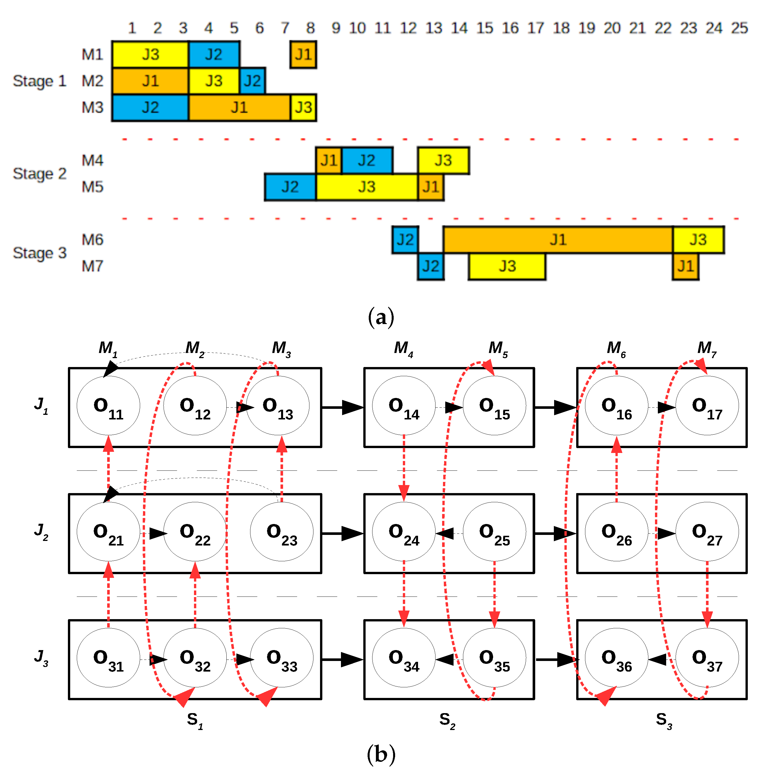
A solution to the FGSSP can be visualized through a classical disjunctive graph representation or a Gantt chart. Figure 1a provides an arbitrary solution to the example problem with ${\sum }_j{C}_j=60$, $C_1=23$, $C_2=12$, $C_3=24$, where $C_j$ is the completion time of job j. The red dotted arcs in Figure 1a show the sequence at the machines and the black dotted arcs show the groups-permutations (i.e., the route of operations for $J_1$ at $S_1$ is $O_{12}$, $O_{13}$ and $O_{11}$ then the route within the stage is $M_2-M_3-M_1$). A Gantt chart representation of the solution is provided in Figure 1b.

The representations in Figure 1a,b show the major characteristics of a FGSSP solution. The disjunctive graph representation visualizes the FGSSP as a sequence of serially arranged OSSP subproblems. Once a job finishes all operations in a stage and then job can start its operations in the subsequent stage. The Gantt chart representation also shows the FSSP behavior among stages. While in the GSSP, a job may have different machines in any given stage, in the FGSSP each job has the same machines in each stage. As a result, the machines of later stages remain idle until operations in preceding stages are completed. These differences motivate the need to separately consider resolution procedures for the FGSSP.

4. FGSSP Formulations and Lower Bounds

This section presents an MILP and a CP formulation for the FGSS problem with total flow time minimization objective and anticipatory sequence-dependent setup times ($FGS{S}_s\mid s_{jik}\mid {\sum }_j{C}_j$). The section also introduces three lower bounds on the value of the optimal objective function. The extension of both formulations for the case without setup times is straightforward, and the changes are described after providing the models with sequence-dependent setup times.

4.1. MILP Formulation

The formulation is an adaptation of the formulation provided in [28] for the $OSS{P}_m\mid S_{jik}\mid {\sum }_j{C}_j$. We now proceed to define the parameters, sets, indices and decision variables of the formulation.

Parameters and Indices:

• $nbJobs$: Number of jobs.
• $nbMchs$: Number of machines.
• $nbStgs$: Number of stages.
• j, k: Indices for jobs, $\{1,\dots ,nbJobs\}$.
• i, l: Indices for machines, $\{1,\dots ,nbMchs\}$.
• s: Index for the stages, $\{1,\dots ,nbStgs\}$.
• $o_{ji}$: Operation associated to job j at machine i.
• $p_{ji}$: Processing time of operation $o_{ji}$.
• $S_{jik}$: Setup time of job j if it is performed immediately after job k on machine i ($j\ne k$).
• $B_{is}$: 1 if machine i belongs to stage s; and 0 otherwise.
• $A_{li}$: 1 if machine l belongs to the stage immediately before the stage to which machine i belongs; and 0 otherwise ($i\ne l$).
• M: A sufficiently large number.

Decision variables:

• $C_j$: Continuous variable that takes the value of the completion time of job j.
• $C_{ji}$: Continuous variable that takes the value of the completion time of job j at machine i.
• $f_{js}$: Continuous variable that takes the value of the completion time of job j at stage s.
• $x_{jil}$: Binary variable that takes value equal to 1 if operation $o_{ji}$ is performed after operation $o_{jl}$; or 0 in any other case.
• $y_{jik}$: Binary variable that takes value equal to 1 if operation $o_{ji}$ is performed after operation $o_{ki}$; or 0 in any other case.

An MILP formulation follows.

$$\begin{array}{cc}\hfill & \min \sum _{j=1}^{nbJobs}{C}_j\hfill \end{array}$$

(1)

$$\begin{array}{cccc}\hfill \mathrm{s}.\mathrm{t}.& C_{ji}\ge p_{ji}\hfill & \hfill & \forall i,j\hfill \end{array}$$

(2)

$$\begin{array}{cccc}\hfill & C_{jl}\ge C_{ji}+p_{jl}-M{x}_{jil}\hfill & \hfill & \forall i,j,l\mid i\ne l\hfill \end{array}$$

(3)

$$\begin{array}{cccc}\hfill & C_{ji}\ge C_{jl}+p_{ji}-M\left(1-x_{jil}\right)\hfill & \hfill & \forall i,j,l\mid i\ne l\hfill \end{array}$$

(4)

$$\begin{array}{cccc}\hfill & C_{ji}\ge C_{ki}+p_{ji}+S_{jik}-M\left(1-y_{jik}\right)\hfill & \hfill & \forall i,j,k\mid j\ne k\hfill \end{array}$$

(5)

$$\begin{array}{cccc}\hfill & C_{ki}\ge C_{ji}+p_{ji}+S_{kij}-M{y}_{jik}\hfill & \hfill & \forall i,j,k\mid j\ne k\hfill \end{array}$$

(6)

$$\begin{array}{cccc}\hfill & C_{ji}-p_{ji}\ge C_{jl}{A}_{li}\hfill & \hfill & \forall i,j,l|i>l\wedge A_{li}=1\hfill \end{array}$$

(7)

$$\begin{array}{cccc}\hfill & f_{js}\ge B_{is}{C}_{ji}\hfill & \hfill & \forall i,j,s\hfill \end{array}$$

(8)

$$\begin{array}{cccc}\hfill & C_j\ge f_{js}\hfill & \hfill & \forall j,s=nbStgs\hfill \end{array}$$

(9)

$$\begin{array}{cccc}\hfill & C_{ji}\in {\mathbb{Z}}^{\ge 0}\hfill & \hfill & \forall i,j\hfill \end{array}$$

(10)

$$\begin{array}{cccc}\hfill & f_{js}\in {\mathbb{Z}}^{\ge 0}\hfill & \hfill & \forall j,s\hfill \end{array}$$

(11)

$$\begin{array}{cccc}\hfill & x_{jil}\in \{0,1\}\hfill & \hfill & \forall i,j,l\mid i\ne l\hfill \end{array}$$

(12)

$$\begin{array}{cccc}\hfill & y_{jik}\in \{0,1\}\hfill & \hfill & \forall i,j,k\mid j\ne k\hfill \end{array}$$

(13)

The objective (1) minimizes the total flow time, i.e., the sum of completion times of the jobs. Constraint set (2) imposes that the completion time of each operation must be larger than the processing time of the job. Disjunctive constraints sets (3) and (4) ensure that each job is not processed in two machines simultaneously. Constraints sets (5) and (6) consider anticipatory sequence-dependent setup times and ensure that each machine does not perform multiple jobs simultaneously. Constraint set (7) defines that the starting time of job j at machine i must be equal to or greater than the completion time of job j at machine l if and only if machine l belongs to the stage immediately before the stage to which machine i belongs. Constraint set (8) calculates the completion time of a job j in a stage s as the maximum completion time of the job j on the machines belonging to the stage. Constraint set (9) computes the flow time of a job as the completion time in the last stage. Finally, constraint sets (10)–(13) define the domain of the decision variables.

Note that while we do not provide a model for the case without sequence-dependent setup times, removing, or setting to 0 the values of, $S_{jik}$ in constraint sets (5) and (6) constitutes a valid model for the case without setup times.

4.2. CP Formulation

As in the MILP case, we develop a CP formulation for the FGSSP problem with total flow time minimization objective and anticipatory sequence-dependent setup times ($FGS{S}_s\mid s_{jik}\mid {\sum }_j{C}_j$). The formulation makes use of several constructs that are available in many CP modeling languages. Specifically, we use interval and sequence variables as well as specific scheduling constraints that are available in the IBM CP Optimizer solver as it is the one used in our our experimental tests.

An interval variable is a construct defined by two variables (the start value and the end value of the interval) as well as a known parameter, the size, that indicates the difference between the end and the start value. A sequence variable is a construct that encodes an ordering of variables. Here, the sequence variables provide an ordering of interval variables corresponding to jobs and machines.

We now proceed to describe the elements of the proposed model.

Parameters and Indices:

• $nbJobs$: Number of jobs.
• $nbMchs$: Number of machines.
• j, k: Indices for the jobs, $\{1,\dots ,nbJobs\}$.
• i, l: Indices for the machines, $\{1,\dots ,nbMchs\}$.
• $o_{ji}$: Operation associated to job j at machine i.
• $p_{ji}$: Processing time of operation $o_{ji}$.
• $A_{li}$: 1 if machine l belongs to the stage immediately before the stage to which machine i belongs; and 0 otherwise ($i\ne l$).
• $T_i$: A transition matrix that reports the minimum delay required by any pair of jobs j, k, to perform in machine i. The transition matrix values equal $S_{jik}$.

Decision variables:

• $itv{s}_{ji}$: Interval variables that define the start and the end of the operation of job j at machine i. The interval variable ensures that the difference between the start and the end value equals the processing time $p_{ji}$.
• $job{s}_j$: Sequence of interval variables $itv{s}_{ji}$ associated to the operations of job j.
• $mch{s}_i$: Sequence of interval variables $itv{s}_{ji}$ associated to operations performed in machine i.

The objective function consists of minimizing the total flow time of jobs, which is computed using the end value of the interval variables:

$$\begin{array}{cccc}\hfill & \min \sum _{j=1}^{nbJobs}{\max }_{i=1}^{nbMchs}endOf\left(itv{s}_{ji}\right)\hfill & \hfill & \hfill \end{array}$$

(14)

where $endOf\left(\right)$ is an integer expression that reports the end of an interval variable. Consequently, ${\max }_{i=1}^{nbMchs}endOf\left(itv{s}_{ji}\right)$ reports the flowtime of job j and (14) provides the total flowtime.

The model contains three constraint sets, (15)–(17).

$$\begin{array}{cccc}\hfill & noOverlap\left(job{s}_j\right)\hfill & \hfill & \forall j\hfill \end{array}$$

(15)

$$\begin{array}{cccc}\hfill & noOverlap\left(mch{s}_i,T_i\right)\hfill & \hfill & \forall i\hfill \end{array}$$

(16)

$$\begin{array}{cccc}\hfill & endBeforeStart\left(itv{s}_{jl},itv{s}_{ji}\right)\hfill & \hfill & \forall i,j,l\mid i>l\wedge A_{l,i}=1\hfill \end{array}$$

(17)

Constraint set (15) ensures that each job j is processed on no more than one machine i at any given time (i.e., since $job{s}_j$ is the subset of operations associated to a job, j $noOverlap\left(\right)$ ensures that the intersection of these intervals is empty).

Constraint set (16) ensures that each machine i does not process more than one job j at a time. Moreover, the transition matrix $T_i$ enforces the setup times between two consecutive operations (the difference between the finalization of an operation and the start of the succeeding operation must be no smaller than their corresponding values in the transition matrix).

Finally, constraint set (17) enforces the stage condition by ensuring that the end of all operations of any given job in a given stage must precede the start of any operation of said job in the next stage.

As in the case of the MILP model, the proposed model can be adapted to the case without sequence-dependent setup times by ignoring setup time values. Here, the change applies to constraint set (16) and the transition matrix of each machine i.

4.3. Lower Bounds

We provide three lower bounds that serve as a basis for comparison of our solution methods. Moreover, as the lower bounds relax some of the conditions of the FGSSP, the gap between the solutions to the FGSSP and the lower bounds may help identify some sources of complexity of the problem, see the results provided in Section 6.

4.3.1. Lower Bound $L{B}_1$

This lower bound considers that the completion time of each job must be no smaller than the sum of its processing times at the machines. Consequently, we can obtain a lower bound by summing the operation time of each job on each machine, see (18). We should expect this bound to be tight when routing decisions are not important, and the stages do not play an important role in the instances, that is, problems where it is possible to obtain solutions without idle times.

$$\begin{array}{cccc}\hfill l{b}_1=& \sum _{j\in J}\sum _{i\in I}{p}_{ji}\hfill & \hfill & \hfill \end{array}$$

(18)

4.3.2. Lower Bounds $L{B}_2$ and $L{B}_3$

$L{B}_2$ and $L{B}_3$ both build upon the relationship of each stage of the FGSSP with the OSSP. As each stage of the FGSSP is an OSSP instance, we can derive a general lower bound by optimally solving (or finding a lower bound) on a OSSP instance with special characteristics (i.e., release dates and delivery times derived from the operation times in the remaining stages).

Consider any stage $s\in \{1,\dots ,nbStgs\}$ and divide the set of stages into three groups, a first group with the stages $\{1,\dots ,s-1\}$ that contains all stages that precede stage s, a second group containing stage s, and a third group with stages $\{s+1,\dots ,s_{nbStgs}\}$ that correspond to the stages following stage s. Clearly, the optimal solution to the OSSP associated to stage s is a lower bound to the objective value of the FGSSP, as it disregards all other stages

Consequently, and to include the remaining stages into the calculation of the lower bound, we estimate the operation times required to complete the operations associated to these stages and associate them to the release dates and delivery times for the OSSP problem in stage s (i.e., we estimate the minimum time unit in which the job can start their operations in stage s and the minimum time required to finish the job once they depart stage s).

The resulting problem corresponds to problem $OSSP\mid r_j,d_j\mid {\sum }_j{C}_j$ or to problem $OSSP\mid r_j,d_j,S_{jik}\mid {\sum }_j{C}_j$ for case without or with sequence-dependent setup times respectively, and the optimal solution, as well as any lower bound of its value is a lower bound for the original FGSSP instance. In order to calculate the bound, we search for a solution to the resulting OSSP model for a limited amount of time using a CP exact solver, see Section 6, and report the optimal solution, if found, or best-known lower bound reported by the solver when the time limit is reached.

The described method provides $nbStgs$ different lower bounds, but we focus our attention on two of these bounds, i.e., the bounds provided by the first and the last stage, as they related problems are easier for the CP solver, and it is more likely that the solver finds the optimal solution, or a better lower bound, for them.

The lower bound for the first stage, $L{B}_2$, corresponds to the optimal resolution of problem $OSSP\mid \mid {\sum }_j{C}_j$, or $OSSP\mid S_{jik}\mid {\sum }_j{C}_j$ for the case with sequence-dependent setup times, plus the sum of operation times in the remaining stages, see Equations (19) and (20), as it is easy to show that the delivery times are constant values that add to the total flow time of the operations independently of the job they are associated to.

$$\begin{array}{cccc}\hfill l{b}_2=& l{b}_{OSSP(s=1)\mid \mid {\sum }_j{C}_j}+\sum _{j\in J}\sum _{i\in I:s\ge 2}{p}_{ji}\hfill & \hfill & \hfill \end{array}$$

(19)

$$\begin{array}{cccc}\hfill l{b}_2=& l{b}_{OSSP(s=1)\mid S_{jik}\mid {\sum }_j{C}_j}+\sum _{j\in J}\sum _{i\in I:s\ge 2}{p}_{ji}\hfill & \hfill & \hfill \end{array}$$

(20)

The lower bound for the last stage, $L{B}_3$ only contains release dates, which may play a role on the optimal schedule of the operations as release dates change the instance where the jobs are available. The resulting bounds correspond to Equation (21), for the case without sequence-dependent setup times, and (22), for the case with sequence-dependent setup times.

$$\begin{array}{cccc}\hfill l{b}_3=& l{b}_{OSSP(s=nbStages)\mid r_j\mid {\sum }_j{C}_j}\hfill & \hfill & \hfill \end{array}$$

(21)

$$\begin{array}{cccc}\hfill l{b}_3=& l{b}_{OSSP(s=nbStgs)\mid r_j,S_{jik}\mid {\sum }_j{C}_j}\hfill & \hfill & \hfill \end{array}$$

(22)

5. Proposed Solution Method

The proposed decomposition-based approach (which we will denote as DEC) exploits the inherent structure of the FGSSP. The structure of a fixed group sShop is similar to the structure of a flow shop but each stage corresponds to an OSSP rather than a single machine. This structure naturally leads to a decomposition in which each Open Shop is individually optimized considering that the sequence of operations on preceding and succeeding stages for each job and on each machine to be known and fixed.

While the approach does not globally optimize the problem, there are intrinsic advantages of the decomposition, specifically, (1) the subproblems do not structurally differ from the original problem and (2) the optimization of each stage allows for minor changes within other stages (i.e., the sequence is fixed but the start time and end time of each operation may vary to accommodate for the changes introduced within the stage under inspection). Moreover, as the sequence of most stages is fixed, the resulting problem is smaller and, supposedly, easier to solve through exact methods. As a result, the proposed method mixes exact and heuristic ideas into a single procedure, a type of method usually referred to as a matheuristic [8] within the literature.

Algorithm 1 provides an outline of the approach. The DEC algorithm creates an initial, incumbent, solution using a constructive heuristic that solves the scheduling problem of each stage sequentially, starting from the first stage, proceeding to the second stage and repeating the process until all $nbStgs$ have been solved. After the initial solution is found, the local search phase is initialized. The local search attempts to improve the solution by solving the subproblems associated to each stage in non-sequential order. If an improving solution is found, the incumbent is updated and the local search is repeated. Otherwise, the incumbent is modified in order to escape from local optimality and the local search phase is called again.

Algorithm 1 gives an overview of the procedure. We now provide details of each step of the DEC method, including an example of the behavior of the algorithm solving the example introduced in Section 3.2.

Algorithm 1: Outline of the DEC procedure.

5.1. Initial Solution

In order to obtain an initial solution to the problem, see lines 3–6 from Algorithm 1, the DEC method starts from an empty solution, and obtains a schedule for the operations of each stage by solving an open shop scheduling problem with release dates and with/without setup times with total flow time objective for each stage (i.e., problem $OSS{P}_m\mid r_j\mid {\sum }_j{C}_j$ or $OSS{P}_m\mid r_j,S_{ij}\mid {\sum }_j{C}_j$, according to [5]).

The procedure starts by obtaining a schedule for the first stage. For this stage, release dates are set to 0. For the remaining stages, stages 2 to $nbStgs$, we solve an OSSP with release dates for each job that are equal to their completion times in their previous stage, These release dates ensure that the operations for any job in a given stage cannot start before the operations of the job finish in previous stages.

Each subproblem is then solved using the model described in Section 4.2 considering only one stage, the stage under consideration, and adding a constraint set, see Equation (23), to impose release dates to the operations associated to each job.

$$\begin{array}{cccc}\hfill startOf\left(itv{s}_{j,l}\right)\ge & r_j\hfill & \hfill & \forall j,l\hfill \end{array}$$

(23)

Constraint set (23) imposes the release date condition by ensuring that the start of any operation cannot be smaller than the release date of the job. In constraint set (23), $r_j$ stands for the release date of job j in the previous stages.

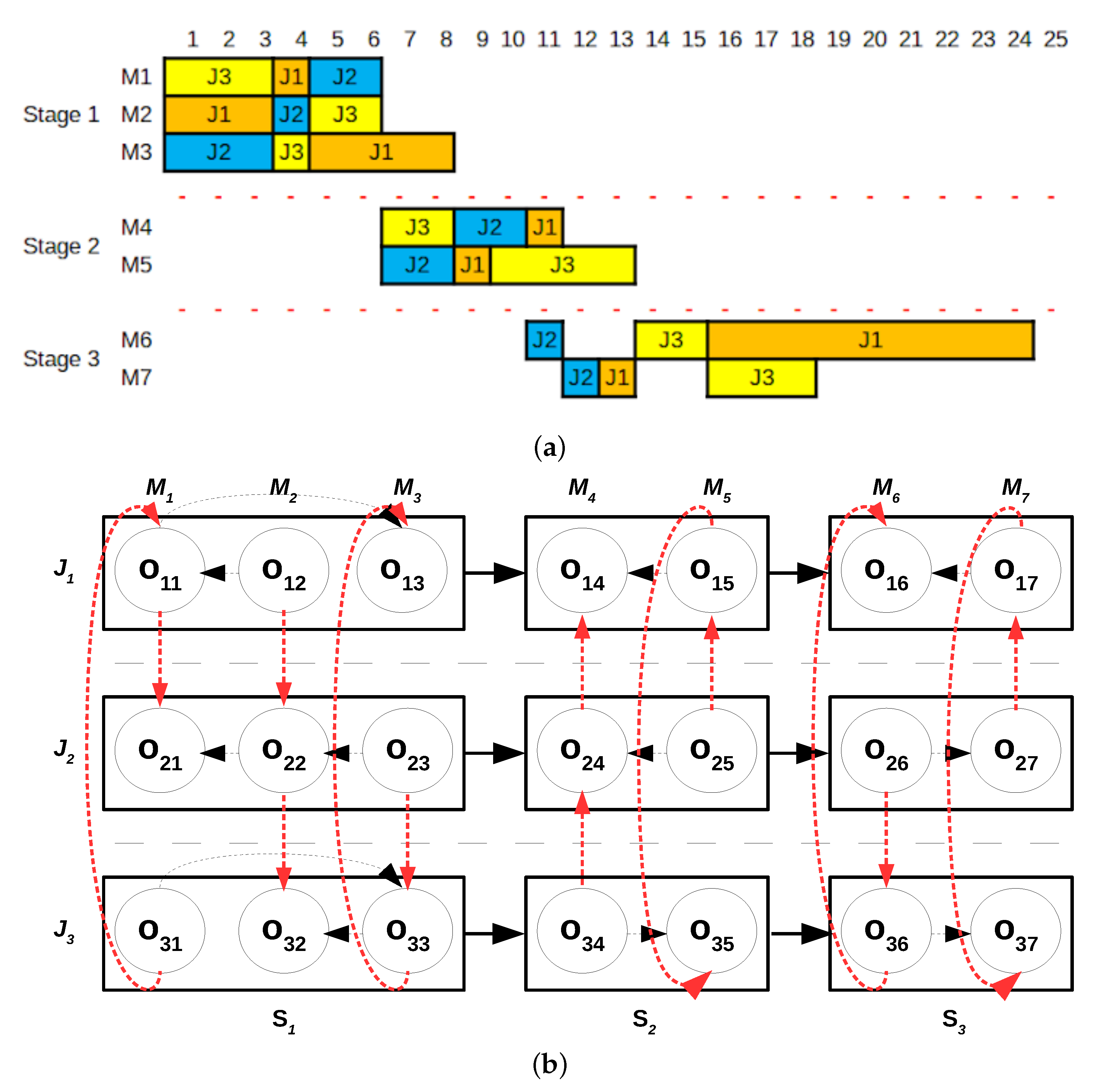
To illustrate the proposed method, let us consider the example introduced in Section 3.2. The construction procedure would start from Stage 1, solving an $OSS{P}_m\mid \mid {\sum }_j{C}_j$ problem with machines M1, M2 and M3. The completion time of the jobs in the optimal schedule correspond to 8, 6 and 6 time units for job 1, job 2 and job 3, respectively. These completion times constitute the release dates for the problem associated with stage 2. In this case, the optimal solution has completion times equal to 11, 10 and 13 for job 1, job 2 and job 3 respectively. Finally, we solve the problem associated to stage 3. The objective function value of the solution provided by the method is 54, Figure 2a shows the Gantt chart of the solution and Figure 2b its disjunctive graph representation.

As the OSSP is a computationally difficult problem by itself, the CP solver is truncated by imposing a time limit. The time limit given to the solver to solve each stage as well as the overall time devoted to the initialization step is controlled through an algorithmic parameter $\alpha$ %, that limits the total time devoted by the algorithm to the step. The time assigned to this step is then evenly divided into each stage to define the time limit set to the CP solver. Note that the time required to reach and to verify the optimal solution of the problem for any given stage may be smaller than the time limit. In this case, the remaining time is reserved for the local search step of the algorithm.

5.2. Neighborhood Exploration

The above constructive procedure provides a feasible solution in which greedy decisions in early stages may have a negative impact on later ones. Consequently, and after an initial solution is available, the neighborhood procedure tries to improve the incumbent by reoptimizing stages, taking into account the scheduling decisions from every other stage, see lines 12–24 from Algorithm 1.

The reoptimization stage is performed as follows: first, we add all stages to a list of pending problems. Then, we randomly select a stage from the list, say, stage s, remove it from the list, and fix the sequence of operations for each job and for each machine in the remaining stages, i.e., each stage $q\in S\backslash \left\{s\right\}$. The resulting model (i.e., the original model with some fixed variables) is then solved using the CP formulation provided in Section 4.2 truncating the search with a time limit which is a parameter of the method. When the time limit is reached or the solver returns that optimality has been verified the best-found solution is compared to the incumbent and the best ever solution

The neighborhood exploration step ends when the list is empty and no improving solution has been found during the last exploration step, in which case we conclude that a local optimum has been found and proceed to restart the local search by slightly altering the solution using the shaking procedure described in Section 5.3. Otherwise, the exploration step is repeated, i.e., the list is initialized with all stages and an optimization problem is solved for each stage, as described above.

To illustrate the proposed method, let us consider the example introduced in Section 3.2, starting from the solution found in Section 5.1 and depicted in Figure 2.

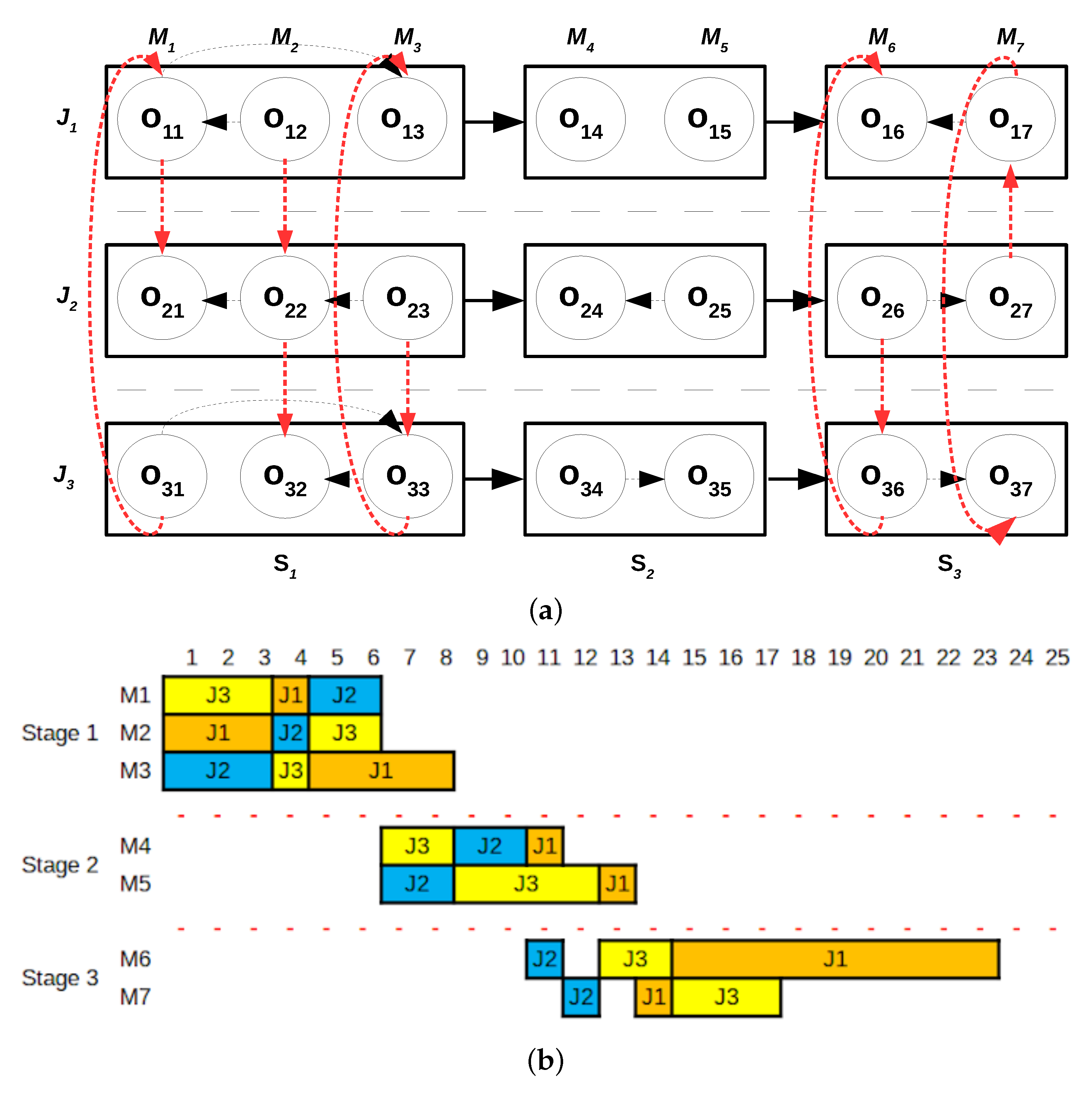
The neighborhood exploration phase starts by initializing the list of pending problems with the three stages. Then, we randomly select a stage from the list. For the sake of this example, let us suppose that stage 2 is selected. Then, stage 2 is removed from the list and a problem with the routes in stages 1 and 3 fixed is given for the CP solver for resolution. Figure 3a gives a disjunctive graph representation of the problem: the routes in stages 1 and 3 are fixed and the problem is allowed to reoptimize the scheduling decisions for stage 2. The optimal solution to the stage 2 problem improves the incumbent as the objective function value is decreased by two time units from 54 to 52 time units, see Figure 3b. The solution also improves the best found solution, hence it replaces both the incumbent, and the best found.

After updating the incumbent, the method would select another random stage among those still in the list, either stage 1 or 3, and build and solve their respective problems. The solutions to either problem do not provide a better solution and thus a complete iteration of the local search ends. As the method has found an improving solution within the last iteration, another iteration of the local search phase is performed. This second iteration does not lead to improvements, hence we conclude that the incumbent is a local optimum and stops the neighborhood exploration step.

Note that each problem solved in this phase is not theoretically easier than the original problem (i.e., they are NP-hard problems). Consequently, and in order to control the total time used within the resolution of the problems, as well as with the complete local search phase, we control both the total time used by the local search phase, and the time allocated to the CP solver to solve each subproblem. Section 6 gives details on the time allotted to each of these parameters in our computational experiments.

Finally, we attempt to improve the performance of the CP solver by providing a “warmstart” solution to it. In this case, we use the incumbent solution from the procedure as it is a feasible solution for the problem, including the additional constraints. As a result, the solver will never provide a worse solution than the initial one, and it will focus the search of areas that may provide improvements over the initial one.

5.3. Shake Procedure

After reaching a local optimum, i.e., the neighborhood exploration step does not improve the incumbent, if the total time limit has not been reached we slightly perturb the solution in order to restart the search from a different position of the solution landscape, i.e., we perform a shake step as in a classical variable neighborhood (VNS) method [36]. Note that the term local optimum in this context is not completely correct, as the truncated nature of our neighborhood exploration scheme may lead us to report that no improving solution has been found when such a solution may exist.

The perturbation scheme considers two randomly-selected consecutive stages and creates an alternative set of routes and assignments for the jobs and the machines in these stages by solving the resulting CP model as in the neighborhood exploration step (i.e., fixing the sequences on the stages that we do not want to modify), but stopping the search when the solver provides a feasible solution and not including the incumbent as a warmstart solution. These decisions help the algorithm to find a solution with enough changes in these stages to move the complete solution away from the current local optimum while the use of the CP model ensures that a solution is found without having to rely on specifically tailored code to ensure feasibility conditions.

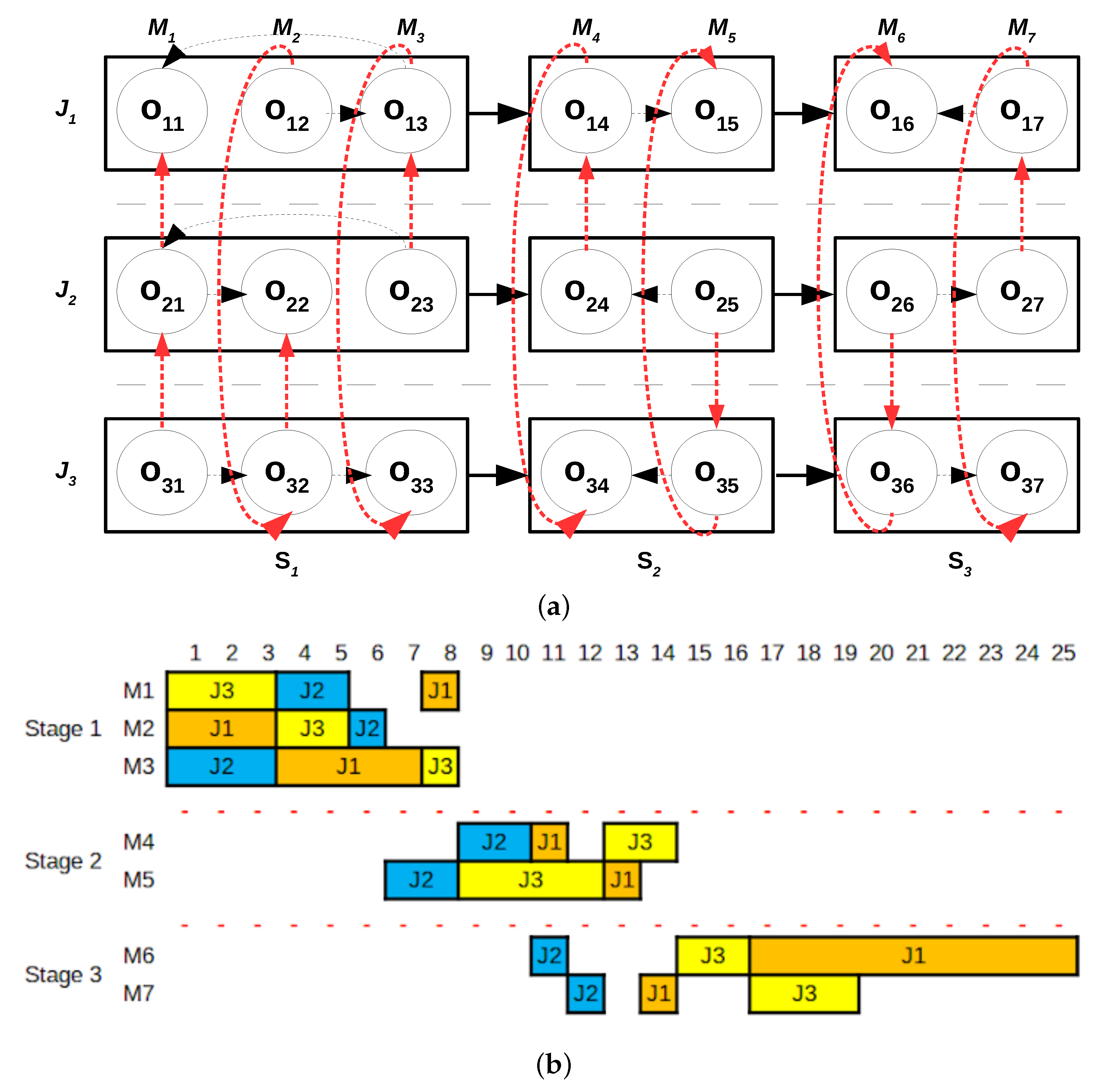
To continue with our example of the proposed method, let us continue with the example introduced in Section 3.2 and used in this Section. After reaching a local optimum, see Section 5.2, the incumbent depicted in Figure 2b is modified by selecting two consecutive stages and generating a random feasible solution for these stages. For the sake of this example, consider that stages 1 and 2 are selected. Then, we solve a problem in which the routes of stage 3 is fixed, and stop the search when the CP solver finds a solution. This solution becomes the incumbent and we return to the neighborhood exploration phase. Figure 4 illustrates the new solution.

6. Computational Experiments

All computational experiments were run on an Intel i7-10750H CPU @2.60 GHz with 6 cores and 16 GB of RAM. The code was written and Java and executed in the Java 8 runtime. The IBM ILOG CP and IBM ILOG CPLEX versions 20.1 were used to solve the CP and MILP formulations. The CP model was solved using five different strategies provided by the solver, namely: Auto (a combined search approach automatically controlled by the solver) CP DF (explores the search tree using a depth-first search approach) RS (combines a depth-first search approach with a restart mechanism after a certain number of backtracking decisions), MP (for multi-point search method, an approach that uses some of the characteristics of a population-based metaheuristic) and ID (for iterative diving search method, an approach that resembles a local search-based heuristic).

Each instance was run with the proposed DEC method with a total CPU time limit equal to $\frac{nbJobsnbMchs}{4}$ seconds, hence we allocate time proportional to the size of the instances. Consequently, for the exact solvers we provide the total time to the solver, while for the DEC approach, the total time allotted to the solution procedure is divided into an initialization phase, that takes a maximum of $\alpha$% of the total time, and the local search phase that takes the remaining time.

During the initialization phase, the resolution of the OSSP associated to each stage is allotted a maximum amount of time equal to $\frac{100}{nbStgs}$% of the total time allotted to this phase (i.e., $\frac{\alpha }{nbStgs}$%). As the allotted time for each subproblem may not be used up ( i.e., the CP solver may report that an optimal solution has been found before the time limit has been reached) the initialization phase may take less than the allotted time. Moreover, it is also possible that the CP solver does not find a solution within the time limit. While this never occurred during our experiments, the default implemented strategy allows the algorithm to continue the search until a feasible solution is found.

During the local search phase, each subproblem is allotted a fixed amount of time equal to $\lambda$. Parameter $\lambda$ controls the trade-off between exploitation and exploration within the local search, i.e., a large value of $\lambda$ has a higher chance to reach an optimal solution for the subproblems at the expense of considering fewer subproblems, while a smaller value of $\lambda$ leads to considering a larger number of subproblems but the CP solver may fail to reach the optimal solution for the subproblem.

After some preliminary tests we opted for $\alpha =0.25$ and $\lambda =\frac{100nbJobsnbMchs}{4nbStgs\left(1-\alpha \right)}$. This value of $\lambda$ should lead to consider each stage no less than three times within the local search phase (our preliminary tests showed that this number usually sufficed to reach the best-found solution and reducing the time to solve each subproblem only lead to degradation in the solution quality).

For the exact methods we impose the following run time limits: For the MILP experiments, we impose a 3600 s time limit, while for the stand-alone CP solver we allocate the same running time as our decomposition approach. Please note that the larger amount of time devoted to the MILP formulation tries to ensure that the performance issues reported in Section 6.2 could not be solved by allocating more computational resources, i.e., running time, to the method.

6.1. Instance Generation

As no previous work for the FGSSP is available in the literature, we generated our own instance set. The generation procedure follows the procedure described in [28] for the $OSS{P}_m\mid S_{jik}\mid {\sum }_j{C}_j$, which extends the procedure described in [37]. Processing times for instances with up to 20 jobs and 20 machines are identical to the processing times used in [37]. For larger instances, the processing times were generated following the indications provided in [37], i.e., they are randomly generated using a discrete uniform distribution $U$ [1,99].

As a result, we generated instances with 4 to 80 jobs, 4 to 80 machines and 2 to 8 stages. In each instance, the first $nbMchs-⌊\frac{nbMchs}{nbStgs}⌋nbStgs$ stages contain $⌈\frac{nbMchs}{nbStgs}⌉$ machines, while the remaining stages have $⌊\frac{nbMchs}{nbStgs}⌋$. We generate 37 groups of instances, each containing 10 instances for a total of 370 instances.

For instances with sequence-dependent setup times we additionally generated setup times as follows: first we generate a random two dimensional Cartesian coordinate $(x,y)$ for each job drawing each coordinate value from a discrete uniform distribution $U$ [0,30]. Then, the setup time between any pair of jobs, j, k, in a given machine is computed as the rectilinear distance between the coordinates associated to each pair of jobs, $|x_j-x_k|+|y_j-y_k|$. This method ensures that setup times comply with the triangle inequality, hence $S_{jik}\le S_{jiu}+S_{uik}$ for any triplet of jobs $j,k,u$ and machine i. Finally, initial setup times were set to 0, i.e., we allow the machines to start working on any job without any setup.

As a result, a total of 740 instances were used for the reported experiments, 370 without sequence-dependent setup times and 370 with setup times.

6.2. Results for Small Size Instances

To evaluate the quality of the solutions provided by the lower bounds and the exact methods introduced in Section 4 we perform two sets of experiments using small instances (those with 10 or fewer jobs and machines) both on the instances with and without sequence-dependent setup times.

The first experiment considers the performance of the exact methods and the DEC procedure. The DEC procedure is run ten times with different random seeds and the results report their average performance among different runs as well as the best solution found within the ten runs.

Table 2. Results for small instances without sequence-dependent setup times (problem $FGSS{P}_s\mid \mid {\sum }_j{C}_j$). For each instance size (represented by the number of jobs, column $nbJobs$, machines, column $nbMchs$, and stages, column $nbStgs$, we report the average gap to the best known solution and the number of best known solutions (in parentheses) provided by each CP search strategy (columns Auto, DF, RS, MP and ID), the best solution provided by all combined CP approaches (column CP), the results from the MILP approach (column MILP) and the best and the average found among 10 independent runs of the DEC approach (columns, (best) and (av.) respectively) using both the MILP and the CP solvers as their underlying methods to tackle the subproblems required by the approach (columns DEC MILP and DEC CP). The results of the best performing method for each group of instances are highlighted in boldface.

										DEC MILP		DEC CP
$\mathit{nbJobs}$	$\mathit{nbMchs}$	$\mathit{nbStgs}$	Auto	DF	RS	MP	ID	CP	MILP	(av.)	(Best)	(av.)	(Best)
4	4	2	0.0 (10)	0.0 (10)	0.0 (10)	0.0 (10)	0.0 (10)	0.0 (10)	0.0 (10)	0.0 (10)	0.0 (10)	0.0 (10)	0.0 (10)
5	5	2	0.0 (10)	1.2 (0)	0.0 (10)	0.4 (4)	0.4 (5)	0.0 (10)	0.0 (10)	0.0 (10)	0.0 (10)	0.0 (10)	0.0 (10)
7	7	2	0.3 (4)	10.3 (0)	0.8 (2)	2.4 (0)	3.7 (0)	0.1 (6)	2.1 (0)	2.7 (0)	2.3 (0)	0.4 (3)	0.3 (4)
		3	0.1 (8)	13.7 (0)	0.3 (7)	1.6 (0)	2.5 (1)	0.0 (10)	0.5 (5)	2.4 (0)	1.9 (1)	2.6 (0)	2.5 (0)
10	10	2	2.2 (1)	14.7 (0)	1.7 (0)	3.7 (0)	3.7 (0)	1.3 (1)	8.9 (0)	11.1 (0)	10.4 (0)	0.5 (3)	0.1 (9)
		3	1.0 (2)	15.8 (0)	1.2 (2)	2.9 (1)	3.1 (0)	0.4 (5)	6.2 (0)	7.4 (0)	7.4 (0)	0.6 (1)	0.5 (5)
		4	1.0 (2)	15.7 (0)	1.1 (1)	1.6 (2)	2.5 (1)	0.4 (6)	3.4 (1)	4.9 (0)	2.9 (2)	1.9 (0)	1.4 (4)

and

Table 3. Results for small instances with sequence-dependent setup times (problem $FGSS{P}_s\mid S_{jik}\mid {\sum }_j{C}_j$). For each instance size (represented by the number of jobs, column $nbJobs$, machines, column $nbMchs$, and stages, column $nbStgs$, we report the average gap to the best-known solution (in parentheses) provided by each CP search strategy (columns Auto, DF, RS, MP and ID), the best solution provided by all combined CP approaches (column CP), the results from the MILP approach (column MILP) and the best and the average found among 10 independent runs of the DEC approach (columns, (best) and (av.) respectively) using both the MILP and the CP solvers as their underlying methods to tackle the subproblems required by the approach (columns DEC MILP and DEC CP). The results of the best performing method for each group of instances are highlighted in boldface.

										DEC MILP		DEC CP
$\mathit{nbJobs}$	$\mathit{nbMchs}$	$\mathit{nbStgs}$	Auto	DF	RS	MP	ID	CP	MILP	(av.)	(Best)	(av.)	(Best)
4	4	2	0.0 (10)	0.0 (10)	0.0 (10)	0.0 (10)	0.0 (10)	0.0 (10)	0.0 (10)	0.0 (10)	0.0 (10)	0.0 (10)	0.0 (10)
5	5	2	0.0 (10)	4.1 (0)	0.0 (10)	0.5 (4)	2.2 (1)	0.0 (10)	0.0 (10)	0.0 (10)	0.0 (10)	0.0 (10)	0.0 (10)
7	7	2	1.4 (1)	15.7 (0)	1.4 (1)	2.3 (1)	4.8 (0)	0.7 (3)	1.4 (2)	2.6 (0)	2.0 (0)	0.3 (3)	0.2 (5)
		3	0.7 (6)	17.3 (0)	0.8 (3)	1.9 (2)	4.2 (0)	0.1 (8)	0.6 (5)	3.1 (0)	2.3 (0)	2.4 (1)	2.3 (1)
10	10	2	4.2 (0)	22.0 (0)	4.3 (0)	5.7 (0)	6.0 (0)	2.8 (0)	9.2 (0)	13.1 (0)	11.3 (0)	0.5 (3)	0.0 (10)
		3	2.2 (3)	23.6 (0)	1.4 (4)	3.9 (1)	5.5 (0)	0.4 (8)	5.4 (0)	7.4 (0)	6.1 (0)	1.5 (0)	1.2 (2)
		4	1.7 (3)	22.3 (0)	1.6 (3)	3.9 (0)	3.6 (1)	0.3 (7)	4.0 (1)	6.1 (0)	4.2 (0)	1.8 (0)	1.3 (2)

report the results. For each solution method, we report the average relative gap $rel.gap$, see Equation (24), in which $UB$ stands for the objective function value reported by the method and $U{B}_b$ corresponds to the best-known objective value among all solution approaches, and, in parentheses, the number of best-known solutions found by the method. For the average performance of the DEC method, $UB$ correspond to the average obtained by the ten independent runs. We also include the results provided by the DEC method using the MILP solver rather than the CP solver for comparison purposes.

$$\begin{array}{cccc}\hfill rel.gap=& 100\frac{UB-U{B}_b}{UB}\hfill & \hfill & \hfill \end{array}$$

(24)

The results in Table 2 and Table 3 show a similar trend, hence we discuss them together pointing out to the differences when needed:

• If we consider the behavior of the exact methods, i.e., the CP variants as well as the MILP, the results show that each of these methods have difficulties even for moderately small instances with 10 jobs and 10 machines. In fact, we do not report the number of optimal solutions found by any of these methods because they fail to verify optimality even for instances with 7 jobs and 7 machines and up. Note that these methods solve all instances with 4 or 5 jobs and machines to optimality, but the combined effort of all the exact methods only verifies optimality for four additional instances.
• Among the different search strategies available in the CP solver, all methods perform similarly except for DF. If we consider this result together with the difficulty of each exact method to verify optimality, we are led to believe that a depth-first search approach as conducted by the DF strategy fails to backtrack to the initial stages of the problem, leading to suboptimal early decision never being reconsidered.
• When we compare the CP approaches and the MILP approach, the CP outperforms the MILP method in every instance group and metric (either number of best found or relative gap to best known). Moreover, the additional time allocated to the MILP does not result in better solutions and the CP approaches, except for the DF strategy, outperform the MILP. Specifically, for instances with 10 jobs and machines, the MILP fails to find solutions of the quality provided by the CP approaches. Consequently, we recommend the use of a CP strategy for the problem and avoid the use of the MILP approach in larger instances.
• The CP methods do not perform as well on instances with sequence-dependent setup times. Specifically, relative gaps increase and two search strategies, i.e., Auto and RS, tend to provide the best solutions among the five search methods. This result may be attributed to shortcomings of the CP approach that makes use of internal components within its search procedure that are more efficient in problems with fewer features to consider.
• The performance of the DEC approach using a CP solver to tackle the subproblems for small and medium instances is similar to the exact CP methods. The same does not hold true for the DEC method using the MILP solver, as their results are inferior to either the CP or the DEC method using CP.
  While the DEC method finds better solutions than the CP methods, specially on instances with fewer stages and the relative gaps are small, it does not outperform the exact methods for these instances. Please note that for small instances, the exact method benefits from considering the problem as a whole, unlike our method that tackles smaller parts of the complete problem. For small sized instances, dividing the problem into part leads to disadvantages in terms of the ability of the method to optimize all stages simultaneously.
  The similarity between the results of both methods was statistically checked using a paired t-test for statistical significance. The paired t-test compares the best solution found by any CP method with the best found among the ten replicates of the DEC method using the CP solver, as well as with each of its individual runs.
  The tests between the best solutions show that the results are not statistically different, with a p-value of 0.204 for the instances without sequence dependent setup times, and a p-value of 0.981 for the case with setup times. Note that Anderson–Darling tests show that the differences among values are not normally distributed, and thus we conduct Wilcoxon signed-rank non-parametric tests that confirm the results from the parametric tests. With regards to the statistical test between individual run of the DEC method when compared to the CP method, similar results are found. For the cases without sequence dependent setup times, six report statistical differences for the parametric test, but after a Bonferroni correction is run to account for multiple comparisons, none of the p-values suffice to point to statistically significant differences. For instances with setup times, none of the replicates report statistically significant differences to the best CP solutions.

To conclude, the results show that the exact methods fail to verify optimal solutions even for moderately small instances, being the CP approaches more competitive in terms of solution quality than their MILP counterparts. While the decomposition scheme can reach solutions of similar quality than the combined effort of all CP methods, and it even outperforms the exact methods for instances with a small number of stages, the results suggest that relying on exact methods is the best approach to solve small-sized instances.

To further analyze the performance of the exact methods, we conducted a second experiment considering the lower bounds introduced in Section 4.3 as well as the lower bounds reported by the CP and the MILP methods after reaching their termination condition, either proving optimality of the incumbent or reaching the imposed time limit.

Lower bounds $l{b}_2$ and $l{b}_3$ require the resolution of an OSSP model which is solved using a CP formulation for a fixed time limit equal to $\frac{nbJobsnbMchs}{4}$ seconds using the default, i.e., Auto strategy, provided by the CP solver. If the time limit is reached without verifying optimality, the lower bound provided by the code is used for the computation of $l{b}_2$ and $l{b}_3$.

Table 4. Results for the lower bounds for small-size instances without sequence-dependent setup times (problem $FGSS{P}_s\mid \mid {\sum }_j{C}_j$). For each combination of instance size (represented by the number of jobs, column $nbJobs$, machines, column $nbMchs$, and stages, column $nbStgs$, and solution method (columns $l{b}_1$, $l{b}_2$, $l{b}_3$, CP and MILP), we report the optimality gap and, in parentheses, the number of instances (out of 10) in which the method reported the best solution. The results of the best performing method for each group of instances are highlighted in boldface.

$\mathit{nbJobs}$	$\mathit{nbMchs}$	$\mathit{nbStgs}$	${\mathit{lb}}_1$	${\mathit{lb}}_2$	${\mathit{lb}}_3$	CP	MILP
4	4	2	21.5 (0)	3.5 (0)	5.0 (0)	0.0 (10)	0.0 (10)
5	5	2	21.4 (0)	3.6 (0)	4.9 (0)	0.0 (10)	0.0 (10)
7	7	2	20.7 (0)	15.7 (2)	12.7 (4)	35.4 (0)	12.7 (4)
		3	24.2 (0)	16.7 (0)	8.9 (0)	21.1 (2)	1.6 (10)
10	10	2	22.1 (0)	17.9 (10)	19.5 (0)	46.2 (0)	40.4 (0)
		3	26.1 (0)	19.3 (10)	22.4 (0)	35.5 (0)	29.3 (0)
		4	28.9 (0)	16.4 (6)	19.7 (3)	32.0 (0)	22.6 (1)

and

Table 5. Results for the lower bounds for small-size instances with sequence-dependent setup times (problem $FGSS{P}_s\mid S_{jik}\mid {\sum }_j{C}_j$). For each combination of instance size (represented by the number of jobs, column $nbJobs$, machines, column $nbMchs$, and stages, column $nbStgs$, and solution method (columns $l{b}_1$, $l{b}_2$, $l{b}_3$, CP and MILP), we report the optimality gap and, in parentheses, the number of instances (out of 10) in which the method reported the best solution. The results of the best performing method for each group of instances are highlighted in boldface.

$\mathit{nbJobs}$	$\mathit{nbMchs}$	$\mathit{nbStgs}$	${\mathit{lb}}_1$	${\mathit{lb}}_2$	${\mathit{lb}}_3$	CP	MILP
4	4	2	28.6 (0)	4.7 (0)	7.2 (0)	0.0 (10)	0.0 (10)
5	5	2	28.6 (0)	5.1 (0)	5.3 (0)	0.0 (10)	0.0 (10)
7	7	2	28.2 (0)	22.7 (0)	20.5 (2)	41.0 (0)	13.9 (8)
		3	31.4 (0)	24.7 (0)	10.9 (0)	34.2 (0)	3.2 (10)
10	10	2	30.6 (0)	26.2 (10)	27.6 (0)	51.8 (0)	44.4 (0)
		3	34.5 (0)	28.3 (9)	30.8 (0)	42.7 (0)	33.9 (1)
		4	36.9 (0)	25.7 (8)	30.8 (0)	39.4 (0)	27.6 (2)

report, respectively, the results for small size instances without and with sequence-dependent setup times.

For each group of instances, we report the results for each lower bound described in Section 4, columns $l{b}_1$, $l{b}_2$ and $l{b}_3$, as well as the best lower bound reported by the CP methods and the MILP model. For each method, we provide two metrics; namely: the optimality gap, calculated as in (25), where $u{b}_b$ is the best known solution and $l{b}_x$ corresponds to the lower bound provided by the method and, in parentheses, the number of instances in which the lower bound provides the best bound among all of the methods.

$$\begin{array}{cccc}\hfill opt.gap=& 100\frac{u{b}_b-l{b}_x}{u{b}_b}\hfill & \hfill & \hfill \end{array}$$

(25)

The results show that large gaps are common. Specifically, for instances with 7 or 10 jobs and machines, the gap after reaching the time limit is very large, hence the inability of the exact solution methods to verify optimality as it cannot prune the search space through tight bounds and has to rely on enumeration to verify optimality. Moreover, the specially tailored lower bounds outperform the general bounds provided by the off-the-shelf solvers. but they still cannot provide tight bounds and the gaps are still large. Finally, we would also like to discuss the differences between the results provided by $l{b}_2$ and $l{b}_3$. While theoretically both bounds should report similar results (we try to optimally solve one stage and estimate the contribution of the remaining stages) the experiments show that $l{b}_2$ usually outperforms $l{b}_3$. We conjecture that this result comes from the performance of the CP solver on the problems solved using this approach. While $l{b}_2$ solves a classical OSSP as a subproblem, $l{b}_3$ solves an OSSP with release dates. The differences may be attributed to a better ability of the CP solver to solve the said subproblem.

To conclude. These results highlight the computational hardness of the problem and the need to rely on specially tailored heuristics to solve large-size instances.

6.3. Results for Medium and Large Size Instances

In this section, we report the results for medium to large-size instances. Due to the results found for small instances, we focus our analysis on solution methods and do not report lower bounds, as the large gaps found for small instances show the difficulty of finding good lower bounds.

Table 6. Results for medium and large instances without sequence-dependent setup times (problem $FGSS{P}_s\mid \mid {\sum }_j{C}_j$). For each instance size (represented by the number of jobs, column $nbJobs$, machines, column $nbMchs$, and stages, column $nbStgs$, we report the average gap to the best solution and the number of instances where the best known solution was found (in parentheses) by the best CP search strategy (column Auto), the best solution provided among the CP approaches (column CP), the results from the MILP approach (column MILP) and the best and the average found among 10 independent runs of the DEC approach (columns, DEC (best) and DEC (av.) respectively). The results of the best performing method for each group of instances are highlighted in boldface.

$\mathit{nbJobs}$	$\mathit{nbMchs}$	$\mathit{nbStgs}$	Auto	CP	DEC (av.)	DEC (Best)
15	15	2	2.9 (0)	2.3 (0)	0.3 (0)	0.0 (10)
		3	1.3 (2)	1.0 (2)	0.5 (3)	0.2 (8)
		4	0.3 (5)	0.3 (7)	1.4 (0)	1.1 (3)
		5	0.7 (4)	0.4 (5)	1.3 (1)	1.0 (5)
20	20	2	3.8 (0)	3.1 (0)	0.2 (3)	0.0 (10)
		3	2.5 (0)	1.9 (0)	0.3 (0)	0.0 (10)
		4	1.9 (2)	1.7 (2)	0.7 (0)	0.1 (8)
		5	1.3 (2)	1.1 (2)	0.8 (0)	0.2 (8)
		6	1.2 (3)	0.8 (4)	1.2 (0)	0.6 (6)
		7	1.0 (2)	0.4 (6)	1.4 (0)	1.0 (4)
30	30	2	5.7 (0)	4.5 (0)	0.0 (5)	0.0 (10)
		3	3.0 (0)	2.9 (0)	0.1 (5)	0.0 (10)
		4	3.5 (0)	2.5 (0)	0.2 (3)	0.0 (10)
		5	2.2 (0)	1.9 (0)	0.5 (2)	0.0 (10)
		6	1.9 (1)	1.6 (1)	0.5 (1)	0.1 (9)
		7	2.0 (1)	1.7 (2)	0.6 (0)	0.0 (8)
50	50	2	8.6 (0)	6.6 (0)	0.0 (2)	0.0 (10)
		3	5.7 (0)	5.4 (0)	0.1 (1)	0.0 (10)
		4	4.5 (0)	4.3 (0)	0.3 (0)	0.0 (10)
		5	4.0 (0)	3.7 (0)	0.1 (0)	0.0 (10)
		6	4.3 (0)	4.0 (0)	0.3 (0)	0.0 (10)
		7	3.3 (0)	3.2 (0)	0.0 (0)	0.0 (10)
		8	3.9 (0)	3.7 (0)	0.4 (0)	0.0 (10)
80	80	2	9.6 (0)	9.6 (0)	0.0 (7)	0.0 (10)
		3	6.9 (0)	6.6 (0)	0.1 (1)	0.0 (10)
		4	5.2 (0)	5.0 (0)	0.2 (1)	0.0 (10)
		5	3.7 (0)	3.6 (0)	0.2 (0)	0.0 (10)
		6	3.5 (0)	3.3 (0)	0.2 (0)	0.0 (10)
		7	3.3 (0)	3.1 (0)	0.3 (0)	0.0 (10)
		8	3.1 (0)	3.1 (0)	0.3 (0)	0.0 (10)

and

Table 7. Results for medium and large instances without sequence-dependent setup times (problem $FGSS{P}_s\mid S_{jik}\mid {\sum }_j{C}_j$). For each instance size (represented by the number of jobs, column $nbJobs$, machines, column $nbMchs$, and stages, column $nbStgs$, we provide the average gap to the best solution and (in parentheses) the number instances where the best CP strategy finds the best known solution (column Auto), the best solution provided among the CP approaches (column CP), the results from the MILP approach (column MILP) and the best and the average found among 10 independent runs of the DEC approach (columns, DEC (best) and DEC (av.) respectively). The results of the best performing method for each group of instances are highlighted in boldface.

$\mathit{nbJobs}$	$\mathit{nbMchs}$	$\mathit{nbStgs}$	Auto	CP	DEC (av.)	DEC (Best)
15	15	2	4.6 (0)	3.2 (0)	0.7 (0)	0.0 (10)
		3	1.6 (1)	1.3 (2)	0.6 (0)	0.1 (8)
		4	1.2 (5)	0.6 (7)	2.5 (0)	1.6 (3)
		5	2.7 (2)	0.4 (6)	1.8 (0)	1.3 (4)
20	20	2	5.0 (0)	4.1 (0)	0.5 (0)	0.0 (10)
		3	4.2 (0)	3.1 (2)	1.1 (0)	0.3 (8)
		4	2.1 (4)	1.1 (4)	2.8 (2)	2.0 (6)
		5	2.7 (1)	0.8 (6)	3.0 (2)	2.5 (4)
		6	2.4 (3)	0.8 (5)	1.2 (0)	0.4 (5)
		7	2.0 (0)	0.5 (4)	1.3 (0)	0.7 (6)
30	30	2	9.6 (0)	7.7 (0)	0.5 (4)	0.0 (10)
		3	5.4 (0)	4.2 (0)	0.5 (0)	0.0 (10)
		4	6.3 (0)	5.3 (0)	1.8 (0)	0.0 (10)
		5	3.4 (1)	3.3 (1)	1.5 (0)	0.2 (9)
		6	3.3 (1)	2.8 (2)	1.2 (0)	0.1 (8)
		7	3.4 (1)	2.5 (1)	1.0 (0)	0.0 (9)
50	50	2	12.6 (0)	8.4 (0)	0.1 (8)	0.0 (10)
		3	7.1 (0)	5.4 (0)	1.0 (0)	0.0 (10)
		4	9.9 (0)	9.1 (0)	1.9 (0)	0.0 (10)
		5	4.8 (0)	4.4 (1)	1.4 (0)	0.1 (9)
		6	6.2 (0)	6.0 (0)	1.1 (0)	0.0 (10)
		7	4.1 (0)	4.0 (0)	0.0 (0)	0.0 (10)
		8	4.7 (1)	4.3 (1)	1.5 (0)	0.4 (9)
80	80	2	14.4 (1)	12.2 (2)	2.0 (2)	1.4 (8)
		3	24.8 (0)	23.5 (0)	1.9 (0)	0.0 (10)
		4	23.2 (0)	21.9 (0)	3.4 (0)	0.0 (10)
		5	21.1 (0)	19.9 (0)	4.1 (0)	0.0 (10)
		6	16.0 (0)	14.0 (1)	3.0 (0)	0.3 (9)
		7	12.4 (0)	11.7 (1)	4.9 (0)	0.1 (9)
		8	14.2 (0)	13.1 (0)	1.9 (0)	0.0 (10)

show average results for these instances grouped according to the number of jobs, the number of machines and the number of stages. The tables compare the results of the best-performing CP strategy, the Auto strategy of the solver, the best solution found among the five search strategies provided by the solver the average result provided by ten independent runs of the DEC method and the best-found solution among these ten independent runs.

The results show similar trends to those found in the small instances (i.e., a deterioration on the performance of the methods when the number of jobs and machines increase). Specifically, for large size instances, the relative gaps increase up to a 9.6% for instances with a small number of stages, and remain above 3% for any number of stages in instances without sequence-dependent setup times. For instances with sequence-dependent setup times, the gaps increase, reporting average relative gaps above 10% on average for any number of stages. These large instances highlight the advantages of the decomposition approach, which is still able to outperform the combined effort of all CP methods in most of the medium-sized and large-sized instances.

While the DEC decomposition approach still relies on a CP solver, the division of the larger problem into smaller subproblems that can be more efficiently tackled in short running times leads to clear improvements over the off-the-shelf method.

The dissimilarity between the results from the CP and the DEC methods were statistically checked using a paired t-test. The paired t-test compares the best solution found by each of the methods.

The test shows that the results are statistically different, with a p-value of $8.79\times {10}^{-31}$ for the instances without sequence dependent setup times, and a p-value of $2.05\times {10}^{-19}$ for the case with setup times. The Anderson–Darling test for normality showed that the differences between the values are not normally distributed, and thus we conduct Wilcoxon signed-rank non-parametric tests to confirm the results from the parametric test. The results of the Wilcoxon tests confirmed the conclusions reached by the parametric tests with a p-value of $7.18\times {10}^{-46}$ for instances without setup times and a p-value of $2.05\times {10}^{-43}$ for instances with setup times.

6.4. An Industrial Case Study

The case study provided below is taken from a Colombian automotive company. The company is dedicated to the manufacturing and assembling of leaf springs that are part of the suspension systems of cars and trucks. The company has over 200 hundred customers and exports to over ten countries. The customers are the car assemblers and the many car and truck repair shops and dealers of the country. A leaf spring consists of “leaves” that are metal plates that are bolted together. Each batch of springs of the same reference is considered a master production order (MPO). In turn, each batch of plates conforming a leaf spring is defined a single production order (SPO) derived from the MPO. Consider a typical reference with 10 plates. If an MPO for 100 leaf springs is issued, a total of 10 SPOs are generated, each with 100 leaf springs. The manufacturing of leaf springs consists of seven stages: (1) plate cutting, (2) center hole drilling and stamping, (3) tempering and quenching, (4) bending, (5) sand blasting, (6) painting and (7) assembly. The assembly operation was not considered in this research as this stage is not really scheduled. All stages have a single machine except stage two that has five forming operations. Stage two is generally the bottleneck station and, for this reason, the company keeps a buffer equivalent to 4–5 days of demand. Each SPO is transferred between workcenters by lift trucks. In this research, jobs correspond to SPOs. The 73 jobs used in this case study correspond to roughly the production of one week, which is the time lapse at which the schedule is revised and updated.

The total number of machines is 16. At the time of writing, there were one cutting station, one drilling machine, ten stamping presses, one tempering/quenching equipment, one bending and adjustment press, one sand blasting equipment and one painting workcenter.

Although the company has and uses an MRP system, the scheduling task is made manually. This is due to the inherent complexity of the manufacturing process and the constant pressure exerted by the vendors of the sales department. Although the company has implemented the Sales and Operations Planning (S and OP) methodology, frequent changes are common on the agreed schedules. For this reason, the company wanted to implement a scheduling system and wanted to test a prototype computer scheduler.

For the tests, we collected data of processing times and production orders from the MRP system. The processing times ranged between 25 min and 5 h depending on the operation. Setups are also important, but the company does not have exact records of the setups. For this reason, we generated setup times based on the suggestions of the plant personnel. Setups are only important in the stamping and drilling operations.

We ran all CP-based algorithms on the proposed instance. The CP DEC was run ten times.

Table 8. Results for case study. For each algorithm the objective value is reported.

Algorithm	Objective Function Value (Minutes)
CP AUTO	263,366
CP DF	293,522
CP RS	274,561
CP MP	293,442
CP ID	264,043
CP DEC (av.)	261,532
CP DEC (best)	260,349

summarizes the results.

As expected, the CP-DEC outperformed the other algorithms showing that the method can also performed well on realistic instances. The best performer among the CPs was the CP AUTO. The difference in terms of the objective function between CP AUTO and CP DEC was around 2200 min per week, which translates into an improvement of 30 min per job (2200/73).

After analyzing the schedule resulting from the CP DEC algorithm, we validated that the bottleneck station (as it is called by the plant personnel) was stage 2. The machine utilizations at this stage ranged from 25% to 78% (average 47%) whereas at the other stages, with the exception of tempering/quenching (66%), was around 30%. These figures of utilization are expected to be higher as the machines are always loaded with jobs from the previous week. We did not have such an information, and therefore we assumed that the factory floor was empty for the purpose of this case. In the experience of the authors, not only the better performance of the scheduling algorithms but also the information they provide, justifies its use.

7. Conclusions and Future Work

In this paper, we introduce fixed group shop scheduling problem (FGSSP) without/with sequence-dependent setup time. The FGSSP is a particular case of the group shop scheduling problem (GSSP) in which the machines of a given stage are the same for all jobs. This case can be found in different settings, as mentioned above.

We describe the characteristics of the proposed problem and provide two formulations, one based on mixed integer linear programming (MILP) and one on constraint programming (CP).

To solve the FGSSP, we developed a novel hybrid heuristic procedure based on a decomposition approach (which we denoted as DEC). Our procedure solves sequentially smaller scheduling problems with CP and presents a simple mechanism to escape from local optima. Moreover, the proposed method can accommodates for additional characteristics required in specific settings by introducing additional constraints within the formulations without the need to modify the solution procedure itself.

To test the performance of the approach, we performed computational experiments where we compare our method to the results provided by off-the-shelf CP and MILP solvers. Additionally, we computed several lower bounds for the FGSSP to have a baseline comparison.

The experimental results show that the DEC and all the tested CP are very similar in terms of performance for small and medium-sized instances, especially when the number of stages is small. For medium and large-sized instances, the DEC outperforms the CP methods with independence of the number of stages, finding the best solution in most of the cases.

Future work will be devoted to studying other solution approaches for the problem, to study the application of the proposed method to similar problems with the proposed approach and to study issues related to Industry 4.0 technologies, such as re-scheduling in the presence of real-time information and rework.

References

- Pinedo, M.L. Scheduling: Theory, Algorithms and Systems, 5th ed.; Springer: New York, NY, USA, 2016. [Google Scholar]
- Zobolas, G.I.; Tarantilis, C.D.; Ioannou, G. Exact, Heuristic and Meta-heuristic Algorithms for Solving Shop Scheduling Problems. In Metaheuristics for Scheduling in Industrial and Manufacturing Applications. Studies in Computational Intelligence, 128; Xhafa, F., Abraham, A., Eds.; Springer: Berlin/Heidelberg, Germany, 2008. [Google Scholar]
- Blum, C.; Sampels, M. An ant colony optimization algorithm for shop scheduling problems. J. Math. Model. Appl. 2004, 3, 285–308. [Google Scholar] [CrossRef]
- Yuraszeck, F.; Mejía, G.; Pereira, J. Modeling and Solving the Total Flow Time Fixed Group Shop Scheduling Problem. In Proceedings of the ICPR Americas, Bahía Blanca, Argentina, 9–11 December 2020; Editorial de la Universidad Nacional del Sur: Bahía Blanca, Argentina, 2020; pp. 2819–2822. [Google Scholar]
- Graham, R.L.; Lawler, E.L.; Lenstra, J.K.; Kan, A.H.G.R. Optimization and heuristic in deterministic sequencing and scheduling: A survey. Ann. Discrete Math. 1979, 5, 287–326. [Google Scholar]
- Rossi, F.; Beek, V.P.; Walsh, T. Handbook of Constraint Programming, 1st ed.; Elsevier Science: Amsterdam, The Netherlands, 2006. [Google Scholar]
- Blum, C.; Raidl, G.R. Hybrid Metaheuristics: Powerful Tools for Optimization, 1st ed.; Springer: New York, NY, USA, 2016. [Google Scholar]
- Maniezzo, V.; Boschetti, M.A.; Stützle, T. Matheuristics: Algorithms and Implementations (EURO Advanced Tutorials on Operational Research), 1st ed.; Springer: New York, NY, USA, 2021. [Google Scholar]
- Masuda, T.; Ishii, H.; Nishida, T. The mixed shop scheduling problem. Discret. Appl. Math. 1985, 11, 175–186. [Google Scholar] [CrossRef] [Green Version]
- Nasiri, M.M.; Kianfar, F. A hybrid scatter search for the partial job shop scheduling problem. Int. J. Adv. Manuf. Syst. 2011, 52, 1031–1038. [Google Scholar] [CrossRef]
- Zubaran, T.K.; Ritt, M. An effective heuristic algorithm for the partial shop scheduling problem. Comput. Oper. Res. 2018, 93, 51–65. [Google Scholar] [CrossRef]
- Ahmadizar, F.; Ghazanfari, M.; Mohammad, S.; Fatemi, T. Group shops scheduling with makespan criterion subject to random release dates and processing times. Comput. Oper. Res. 2010, 37, 152–162. [Google Scholar] [CrossRef]
- Ahmadizar, F.; Rabanimotlagh, A. Group shop scheduling with uncertain data and a general cost objective. Int. J. Adv. Manuf. Technol. 2014, 70, 1313–1322. [Google Scholar] [CrossRef]
- Ahmadizar, F.; Shahmaleki, P. Group-shop scheduling with sequence-dependent set-up and transportation times. Appl. Math. Model. 2014, 38, 5080–5091. [Google Scholar] [CrossRef]
- Kemmoé-Tchomté, S.; Féniès, P.; Lamy, D.; Tchernev, N. A Multi-start Multi-level ELS for the Group-Shop Scheduling Problem. IFAC-PapersOnLine 2018, 51, 1299–1304. [Google Scholar] [CrossRef]
- Liu, S.Q.; Ong, H.L.; Ng, K.M. A fast tabu search algorithm for the group shop scheduling problem. Adv. Eng. Softw. 2005, 36, 533–539. [Google Scholar] [CrossRef]
- Nasiri, M.M. A modified ABC algorithm for the stage shop scheduling problem. Appl. Soft Comput. 2015, 28, 81–89. [Google Scholar] [CrossRef]
- Nasiri, M.M.; Kianfar, F. A GA/TS algorithm for the stage shop scheduling problem. Comput. Ind. Eng. 2011, 61, 161–170. [Google Scholar] [CrossRef]
- Nasiri, M.M.; Hamid, M. The stage shop scheduling problem: Lower bound and metaheuristic. Sci. Iran. 2020, 27, 862–879. [Google Scholar] [CrossRef] [Green Version]
- Ahmadizar, F.; Ghazanfari, M.; Fatemi Ghomi, S.M.T. Application of chance-constrained programming for stochastic group shop scheduling problem. Int. J. Adv. Manuf. Syst. 2009, 42, 321–334. [Google Scholar] [CrossRef]
- Nie, X.D.; Chen, Y.P.; Yang, Y.J. The Cyclic Scheduling of Material Transporting Robot in Group Shop. Appl. Mech. Mater. 2012, 263–266, 634–638. [Google Scholar] [CrossRef]
- Ahmadizar, F.; Zarei, A. Minimizing makespan in a group shop with fuzzy release dates and processing times. Int. J. Adv. Manuf. Syst. 2013, 66, 2063–2074. [Google Scholar] [CrossRef]
- Ahmadizar, F.; Rabanimotlagh, A.; Arkat, J. Stochastic group shop scheduling with fuzzy due dates. J. Intell. Fuzzy Syst. 2017, 33, 2075–2084. [Google Scholar] [CrossRef]
- Sampels, M.; Blum, C.; Mastrolilli, M.; Rossi-doria, O. Metaheuristics for Group Shop Scheduling. In Proceedings of the LNCS 2439, PPSN VII, Granada, Spain, 7–11 September 2002; Merelo Guervós, J.J., Adamidis, P., Beyer, H.-G., Schwefel, H.-P., Fernández-Villacañas, J.-L., Eds.; Springer: Berlin/Heidelberg, Germany, 2002; pp. 631–640. [Google Scholar]
- Zhou, J. A Permutation-Based Approach for Solving the Job-Shop Problem. Constraints 1997, 2, 185–213. [Google Scholar] [CrossRef]
- Malapert, A.; Cambazard, H.; Guéret, C.; Jussien, N.; Langevin, A.; Rousseau, L.M. An optimal constraint programming approach to the open-shop problem. INFORMS J. Comput. 2012, 24, 228–244. [Google Scholar] [CrossRef] [Green Version]
- Lunardi, W.T.; Birgin, E.G.; Laborie, P.; Ronconi, D.P.; Voos, H. Mixed Integer Linear Programming and Constraint Programming Models for the Online Printing Shop Scheduling Problem. Comput. Oper. Res. 2020, 123, 105020. [Google Scholar] [CrossRef]
- Mejía, G.; Yuraszeck, F. A self-tuning variable neighborhood search algorithm and an effective decoding scheme for open shop scheduling problems with travel/setup times. Eur. J. Oper. Res. 2020, 285, 484–496. [Google Scholar] [CrossRef]
- Meng, L.; Lu, C.; Zhang, B.; Ren, Y.; Lv, C.; Sang, H.; Li, J.; Zhang, C. Constraint programing for solving four complex flexible shop scheduling problems. IET Collab. Intell. Manuf. 2021, 3, 147–160. [Google Scholar] [CrossRef]
- Meng, L.; Zhang, C.; Ren, Y.; Zhang, B.; Lv, C. Mixed-integer linear programming and constraint programming formulations for solving distributed flexible job shop scheduling problem. Comput. Ind. Eng. 2020, 142, 106347. [Google Scholar] [CrossRef]
- Dorndorf, U.; Pesch, E.; Phan-Huy, T. Constraint propagation and problem decomposition: A preprocessing procedure for the job shop problem. Ann. Oper. Res. 2002, 115, 125–145. [Google Scholar] [CrossRef]
- Maravelias, C.T.; Grossmann, I.E. A hybrid MILP/CP decomposition approach for the continuous time scheduling of multipurpose batch plants. Comput. Chem. Eng. 2004, 28, 1921–1949. [Google Scholar] [CrossRef]
- Sacramento, D.; Solnon, C.; Pisinger, D. Constraint Programming and Local Search Heuristic: A Matheuristic Approach for Routing and Scheduling Feeder Vessels in Multi-terminal Ports. SN Oper. Res. Formu 2020, 1, 32. [Google Scholar] [CrossRef]
- Fazel Zarandi, M.H.; Sadat Asl, A.A.; Sotudian, S.; Castillo, O. A state of the art review of intelligent scheduling. Artif. Intell. Rev. 2020, 53, 501–593. [Google Scholar] [CrossRef]
- de Abreu, L.R.; Guimara es Araújo, K.A.; de Athayde Prata, B.; Nagano, B.S.; Moccellin, J.V. A new variable neighbourhood search with a constraint programming search strategy for the open shop scheduling problem with operation repetitions. Eng. Opt. 2021. [Google Scholar] [CrossRef]
- Hansen, P.; Mladenović, N. Variable Neighborhood Search. In Handbook of Heuristics; Martí’, R., Pardalos, P.M., Resende, M.G.C., Eds.; Springer: Berlin/Heidelberg, Germany, 2018. [Google Scholar]
- Taillard, E. Benchmarks for basic scheduling problems. Eur. J. Oper. Res. 1993, 64, 278–285. [Google Scholar] [CrossRef]
Figure 1.
Graphical representations of a solution to the example instance provided in Table 1. (a) Gantt chart representation of an arbitrary feasible solution for the FGSSP instance presented in Table 1 with . (b) Disjunctive graph representation of an arbitrary feasible solution for the FGSSP instance presented in Table 1 with .
Figure 2.
Graphical representation of the constructive heuristic solution of the DEC method for the example instance provided in Table 1. (a) Gantt chart representation of the solution provided by the constructive heuristic for the FGSSP instance presented in Table 1. (b) Disjunctive graph representation of the solution provided by the constructive heuristic for the FGSSP instance given in Table 1.
Figure 3.
Graphical representation of the neighborhood exploration phase of the DEC method for the example instance provided in Table 1. (a) Disjunctive graph representation of the problem associated to the stage 2. The arcs represent the fixed decisions (i.e., the decisions from stage 1 and 3). (b) Gantt chart representation of the solution after solving the problem of stage 2. The solution improves the problem by rearranging the order of operations of the stage.
Figure 4.
Graphical representation of the incumbent solution of the DEC method after the shake is performed for the example instance provided in Table 1. (a) Disjunctive graph representation of the incumbent solution after the shake. (b) Gantt chart representation of the incumbent solution after the shake.