An Efficient Point-Matching Method Based on Multiple Geometrical Hypotheses
by
 , , ,
, , ,
Miguel Carrasco
1 ,
,
Domingo Mery
2 ,
,
Andrés Concha
1, 
Ramiro Velázquez
3 ,
,
Roberto De Fazio
4 and
Paolo Visconti
4,* 1
Facultad de Ingeniería y Ciencias, Universidad Adolfo Ibáñez, Peñalolén, Santiago 7941169, Chile
2
Departamento de Ciencia de la Computación, Pontificia Universidad Católica de Chile, Santiago 7820436, Chile
3
Facultad de Ingeniería, Universidad Panamericana, Aguascalientes, Aguascalientes 20290, Mexico
4
Department of Innovation Engineering, University of Salento, 73100 Lecce, Italy
*
Author to whom correspondence should be addressed.
Electronics 2021, 10(3), 246; https://doi.org/10.3390/electronics10030246
Submission received: 30 December 2020
/
Revised: 15 January 2021
/
Accepted: 18 January 2021
/
Published: 22 January 2021
(This article belongs to the Special Issue Applications of Computer Vision)
Abstract
:Point matching in multiple images is an open problem in computer vision because of the numerous geometric transformations and photometric conditions that a pixel or point might exhibit in the set of images. Over the last two decades, different techniques have been proposed to address this problem. The most relevant are those that explore the analysis of invariant features. Nonetheless, their main limitation is that invariant analysis all alone cannot reduce false alarms. This paper introduces an efficient point-matching method for two and three views, based on the combined use of two techniques: (1) the correspondence analysis extracted from the similarity of invariant features and (2) the integration of multiple partial solutions obtained from 2D and 3D geometry. The main strength and novelty of this method is the determination of the point-to-point geometric correspondence through the intersection of multiple geometrical hypotheses weighted by the maximum likelihood estimation sample consensus (MLESAC) algorithm. The proposal not only extends the methods based on invariant descriptors but also generalizes the correspondence problem to a perspective projection model in multiple views. The developed method has been evaluated on three types of image sequences: outdoor, indoor, and industrial. Our developed strategy discards most of the wrong matches and achieves remarkable F-scores of 97%, 87%, and 97% for the outdoor, indoor, and industrial sequences, respectively.
1. Introduction
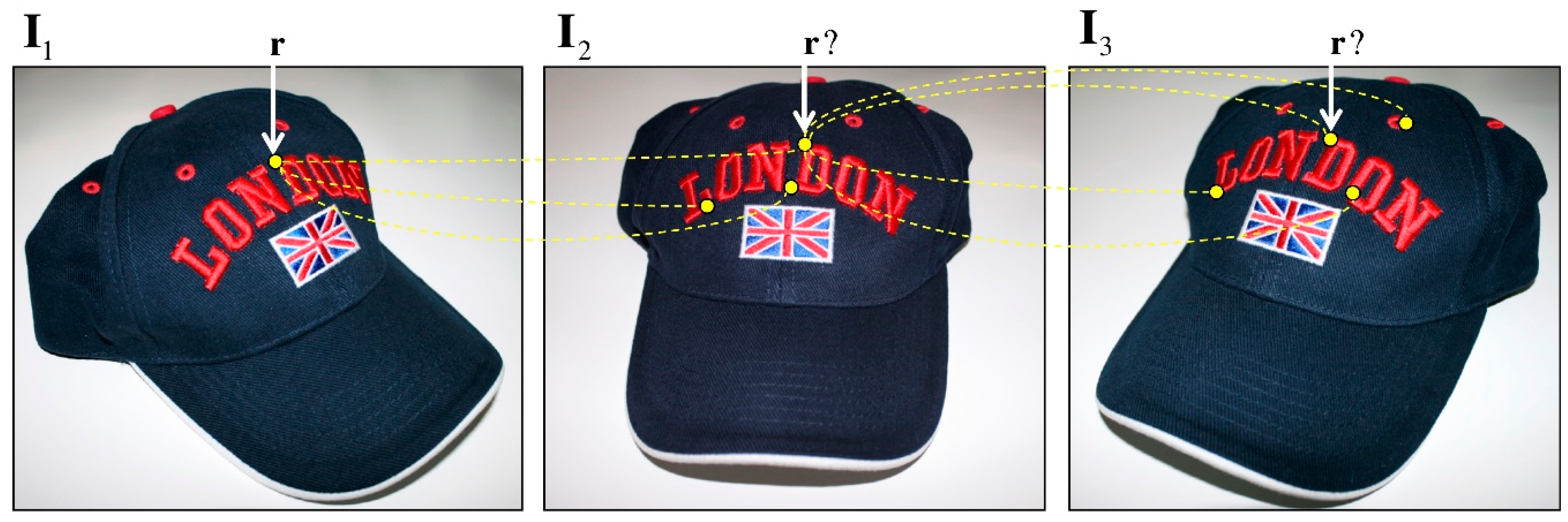
Point matching in two or more images is a very relevant and complex problem in computer vision. It finds applications in robot navigation, 3D object reconstruction, multiple-view tracking, and homography, among others. It basically consists of identifying a set of points across several images. The problem definition is shown in Figure 1.
Due to the different points of view from which the images were captured, the corresponding points might exhibit differences across the images. Such differences are mainly due to the geometric transformations and photometric conditions determined by the continuous motion of both object and cameras [1]. In addition, it is possible to have different textures and colors among the points whose correspondence is trying to be established. Therefore, wrong matches are likely to arise and degrade the correspondence results.
The analysis of the invariant descriptors is considered the general approach to find point correspondence. By using invariant descriptors, you can resolve the point-matching problem by extending the methods commonly used in stereovision. Normally, the correspondence is determined from the points of interest (PoI) previously obtained by an algorithm able to detect the regions of interest (RoI) [2,3,4]. However, when the current saliency techniques [5,6,7,8] cannot detect the PoI, determining its matching pair or triplet into other images becomes a difficult task. In this case, the previously proposed methods cannot ensure proper correspondence because they are able to maximize their performance solely in the detected RoIs and not perforce in other regions. In addition, for image sequences exhibiting low signal to noise ratio (SNR), they will not work very well because of the false alarms [9]. For the above reasons, the problem of finding correct (or incorrect) matches is still an open problem in computer vision.
This paper introduces an efficient point-matching method capable of filtering most of the wrong correspondences. In order to achieve this task, a proper combination of multiple partial solutions by means of an invariant and a geometrical analysis is proposed. Graphically, once a point r in the image I1 has been determined, then the aim is to find the corresponding point in the image I2; indeed, only one possibility is correct. However, when an analysis of the characteristics is employed, other regions can also be candidates for such correspondence, for example, when the corresponding point is not appearing due to an occlusion. Before using a third image I3, to solve the problem it is necessary to consider that the correspondence for the first two images has been already solved. Since the method uses a perspective projection model that is object-independent, it is possible to determine the corresponding point’s position also in those views where it is occluded [10]. Most of the research in this area is focused on reducing the general error of control points, and selecting a stable subset of points, discarding a large part of partial solutions, which, although correct, are discarded in the final solution. Our proposal uses each of the partial solutions in a way that considers the error within the final solution. The main advantage of our proposal is to take advantage of partial solutions and weight them according to the error they have. The smaller the estimation error, the greater its final weight in the reprojection estimate. A preliminary version of this idea was presented in [11] but only for two views. In this paper, we generalize the problem by analyzing up to three images (Figure 1).
The remainder of the paper is structured in five sections. Section 2 overviews the main concepts related to the multiple view analysis. Section 3 provides a comprehensive description of the proposed method. Section 4 presents the experiments and results obtained. Finally, Section 5 concludes the paper and gives future work perspectives.
2. Background
Over the last 20 years, different methods for addressing the point-matching problem have been proposed. Methods and techniques based on the analysis and optimization of the invariant descriptors [12,13,14], estimation of affine transformations/homographies/perspective transformations [15,16,17], epipolar geometry analysis [18,19,20], optical flow-based methods [21,22], and methods based on geometric and photometric constraints [4,23] are some of the approaches already explored.
Overall, the abovementioned methods’ performance relates to the type of motion the objects exhibit in a video sequence. For static scenes without any camera motion, the problem is basically reduced to analyzing the epipolar geometry of the two images using stereovision [24]. For dynamic images, if the objects are subjected to small displacements, optical flow-based techniques have shown to be efficient at determining correspondences [25]. However, if the objects undergo large displacements, the same optical flow-based techniques will not perform well as they were not designed for such cases.
2.1. Problem Definition for Two Views
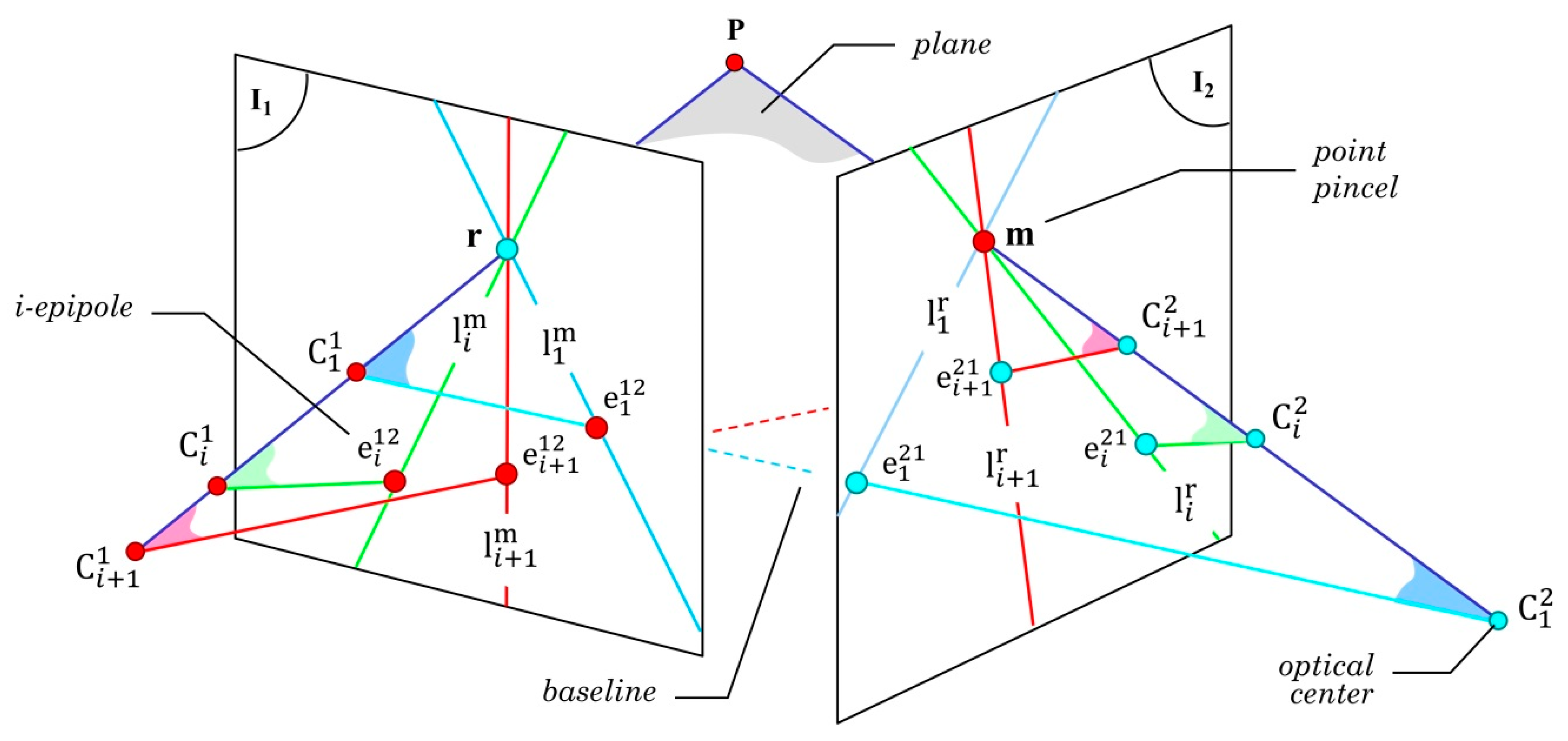
The geometric relationship between the two corresponding images is one of the most studied topics in computer vision. The purpose is to determine correctly the geometric relations of a point in the 3D space as well as its projections on the 2D planes (Figure 2). The first step to be executed towards a solution is to find a set of point-correspondences that represent the geometric relationships between the images [26].
Let P be a 3D point located at the upper corner of the 3D cube (Figure 2). We indicate with C1 and C2 the optical centers of the cameras providing the two different viewpoints. Let us assume that two images were captured from the optical centers C1 and C2 generating images I1 and I2, respectively. Accordingly, if two rays are projected from points C1 and C2 to point P, two new points (indicated as r and m in Figure 2) are generated on the 2D plane of images I1 and I2, respectively. This relationship determines that both rays intersect at point P and that their projections can be safely placed on the I1 and I2 planes. In this way, r and m belong to a projection of the point P generated from the optical centers (C1, C2). Ideally, since both points were generated from point P, they are corresponding. On the contrary, if the existence of point P is unknown, the existence of the correspondence cannot be assured. This last situation usually happens in the point-to-point correspondence problems.
The fundamental matrix F is a conventional way to demonstrate the relationship between r and m [18,27]. F contains the intrinsic geometry of the two views, named the epipolar geometry. To determine F, certain knowledge on a minimum set of matching points in both views is required [28,29]. This could be done with the NNDR (nearest neighbor distance ratio) algorithm for analyzing each feature descriptor for every point [30]. Formally, given a pair }, where indicates matching points, it always satisfies the following epipolar restriction: , where and are in homogeneous coordinates. Nevertheless, this relation stands true for all the points located at the intersection of the projection plane of C2 and I2 (Figure 2). Such intersection generates a line called epipolar line [26]. Since point m belongs to the plane of C2, it can be said that the epipolar line, in the second view I2, corresponds to the point r in the first view I1. Accordingly, a bi-univocal relationship between the points r and m cannot be determined using only one epipolar line, i.e., the position of m from r cannot be determined; therefore, , where indicates a hypothetical match, that at least does fulfill the epipolar restriction.
Let us now assume that r and m are corresponding points. As they belong to the same plane, they are therefore located on the epipolar lines and . That is, and . In practice, both views’ measurements are not very precise, implying that the epipolar lines and the corresponding points do not necessarily intersect. Mathematically, this means that and [26]. The Euclidian distances, called and , in which and , reflect such error (see Figure 2).
To obtain correct projections, both distances and , should be minimal. For this purpose, the distance between the real position of the point and the projected epipolar line’s position should be minimized. In some cases, the error is caused by the optical distortions related to the camera’s lenses or by additive Gaussian noise generated during the acquisition step of the coordinates in correspondence, resulting in slight matching errors that reduce the accuracy of the geometric projection model.
2.2. Problem Definition for Three Views
A three-view analysis allows the modelling of the geometric relations that take place in the 3D space [31]. Figure 3 shows an example. Here, the relationship between the projection of a 3D point and the three bi-dimensional projection planes is illustrated. The projection of the point P on the I1, I2, and I3 planes produces the corresponding r, m, and s projections in each image. The perspective projection model is valid for the point even in situations in which the projection is not visible, either because the point is blocked or it is located out of the field of view of the camera. The use of the matrix tensor called Trifocal tensor [26] is thus needed to perform an estimation. One of the Trifocal tensor’s main advantages is that it depends solely on the motion between the views and on the cameras’ internal parameters. It is completely defined by the projection matrices of which it is constituted. Moreover, the Trifocal tensors can be calculated by means of the correspondences of images without any prior knowledge of the under-analysis object. Hence, the analysis can be reduced to estimate the projection matrices error by using the set of correspondences in the three views.
Formally, the trifocal tensor is a 3 × 3 × 3 matrix comprising the relative motion between the three views I1, I2, and I3 (see some examples in [26,32]). As mentioned above, one of its most significant features is that, upon its estimation, it is possible to find the position of a point s in the I3 plane by using the positions of the correspondences of the first and second views, respectively, as depicted in Figure 3. The re-projection is defined in terms of the r and m positions in homogeneous coordinates and of T, derived from the first two tri-linearities of Shashua [33]. For such purpose, let be the Trifocal tensor projection in the third view; is defined as in homogenous coordinates. Unfortunately, the estimation of is subject to an error determined by two causal factors: (1) an incorrect choice relative to the set of correspondences or (2) a correspondence error between the r and m pairs. Figure 3 does not illustrate the latter case; however, most of the correspondences encompass that type of error. Even if the tensors are relatively stable in the image sequences, as happens in the ideal case, however, there is always an error between the hypothetical correspondence s and the re-projected point . For simplicity, let us define the distance between these points as the Euclidian distance of the point, indicated as and calculated as follows: .
The process of estimating T ends typically with the reduction of some error metrics, such as minimizing the distance from multiple random solutions or modelling the error as a probability distribution. Anyway, for each estimation of T, there is only one possible projection associated with each pair of correspondences . Assuming that other random solutions are also valid, the ultimate goal will be to correctly estimate each re-projection’s error. The error associated with each selection of T will be employed, later in the process, in order to re-estimate the re-projection distances of point s in the third view, similarly to the determined error of the distance to the epipolar line.
2.3. Research Justification
So far, methods for obtaining F and T have focused on using an error minimization process to determine the best model as generated from a set of random pairs in correspondence [34,35,36,37]. Such a minimization process normally takes place by using a consensus sampling technique known as random sample consensus (RANSAC) [34], MLESAC’s likelihood maximization by random sampling [35], and more recently by the ARSAC method [36]. All these proposed methods, as well as the obtained improvements reported in [37,38], have demonstrated to be efficient at finding the fundamental matrices and trifocal tensors in computer vision problems.
In two views, the main purpose of the minimization process is to correctly determine a single epipolar line with the aim of finding an optimum epipole [18,39]. Proposed methods have been developed for situations in which there is an important number of wrong correspondences. To reduce the selection of wrong correspondences, the random search for hypotheses aims to determine the quality of each selected hypothesis [40,41].
A similar idea suggested by Sur et al. [23] proposes a point-matching method based on the proper combination of photometry and camera geometry estimates in two views. Nonetheless, the main difference with our method is that Sur’s is designed to find the most consistent set and then estimate camera motion geometry in a way that improves the RANSAC algorithm.
What happens when it is found a high number of correctly estimated correspondences has not been addressed. Whether or not the best hypothesis can be considered, the only solution has not been answered either. This work presents a new innovative method to determine the point-to-point correspondence in two and three views, so addressing these two open questions.
3. Point-Matching Method Based on Multiple Geometrical Hypotheses
The estimation of F is strongly dependent on the set of correspondences employed. For every set of correspondences, a new F is determined. Each set requires a minimum number of corresponding points in the two views. Even if the fundamental matrices are different, they all remain valid for . The employment of multiple fundamental matrices exhibits two main advantages: (1) every new F defines a new epipole position in the planes I1 and I2. (2) The intersection between the epipole and the hypothetical point in correspondence, r or m, creates a new epipolar line.
Considering these properties, the method herein presented proposes to select k subsets extracted from the input matches. Formally, for each , the i-th subset is defined by the random choice of n corresponding points. According to Figure 4, the and epipoles are defined as the intersection points between the baseline of optical centers and and the I1 and I2 planes, respectively. Thus, for every image, there is an epipole (not necessarily visible) in the plane. For the proposed model, as shown in Figure 4, it is assumed that the point P is fixed.
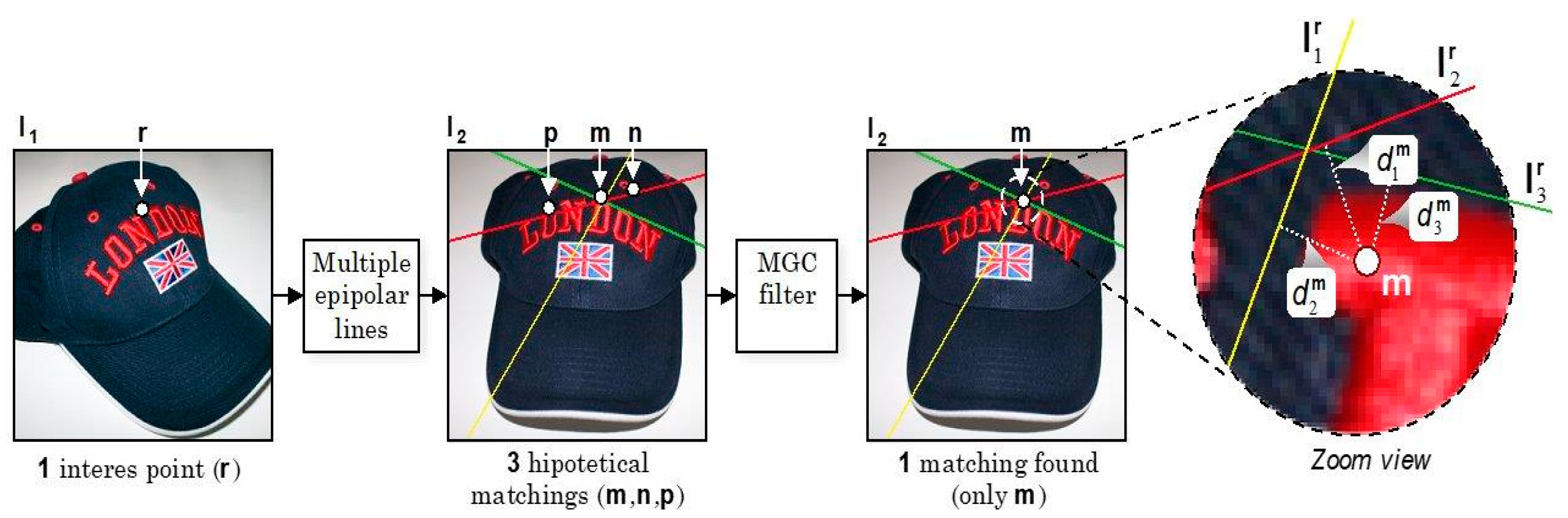
To illustrate the correspondence estimation process in two views, it will be further assumed that there is always a corresponding point in the second view, once defined a point r in the first view. Since such correspondence is unknown, it will be assumed that there are three hypothetical corresponding points: m, n, and p. Figure 5 shows the first set of correspondences in which the epipolar line intersects the points m, n, and p, in the plane I2.
Let be the set of known hypothetical correspondences in the two views. If we intersect and , both generated by two sub-sets of correspondences different from each other, it can be clearly seen that the line is considerably far away from the correspondences n and p. Likewise, a third epipolar line intersects the two previous ones at the point m, because the set of projected epipolar lines of point r intersects only one corresponding point in the second view, which in this case is the point m, thus generating a point pincel, namely, a point where multiple lines intersect among them. Both images exhibit that effect, as shown in Figure 4.
Although it seems that every new epipolar line determines an increase of the corresponding point’s precision, actually there is no single intersection point due to the nature of the corresponding points employed to formulate the perspective projection model, resulting in an error in the estimation of each fundamental matrix. The main inconvenient of estimating epipolar lines is the need to determine their error level. The error is clearly not the same in all epipolar lines; hence, a method is required to determine the errors associated with the Euclidian distance of each epipolar line.
Let define as the Euclidian distance between the m-th point of the second view and the epipolar line , with r representing the r-th point of the first view for all subset. The distance can be expressed by Equation (1):
where is the c-th component of the vector . The primary goal is to determine the correct pair of the set Φ or in plain words, so that to select the pair and consequently to discard the incorrect pairs and . Still, the estimation error related to each epipolar line is unknown. To perform such estimation, the MLESAC algorithm can be used [35]. The purpose of this method is to recalculate the Euclidian distances , , and weighting the error of each epipolar line. This procedure will be described in the next section.
3.1. Multiple Trifocal Tensors
This section presents a similar analysis now considering three views. The use of four or even more views does not necessarily increase the method’s performance, as it depends on the application type in which the matching procedure is framed. Our belief is that a third view is able to reduce the remaining false alarms since the probability that they remain in their relative position in all three views is very low.
Again, the proposed framework uses the re-projection from the multiple projections’ estimation of potential matching features in two perspectives. We estimated the error to properly weigh the re-projected point’s distances in the third sight compared to the positions of hypothetical correspondences. A selection of random sets of corresponding features is employed again to calculate each trifocal tensor’s solution. The RANSAC framework would generally reject the intermediate results and consider a group featured by slightest re-projection error. In this problem, a reduced estimation error is produced by the group of corresponding random features. Hence, the algorithm can employ multiple valid set of correspondences, obtained similarly to the estimation of several fundamental matrices.
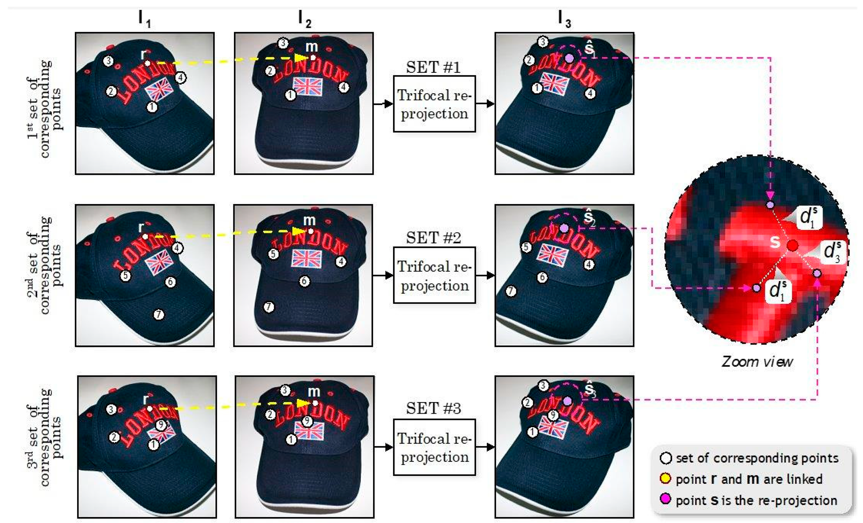
Next, the estimation of the perspective projection model with three views is briefly discussed. In the following Section 3.2, Figure 6 and Figure 7 illustrate an application example of the technique. Three sets of independent correspondences are considered. Each of which produces the re-projection of the tensor in the third view (i.e., in the , , and positions). By extending the above example, for each i subset, the trifocal tensor Ti, for all is estimated [26,28,42]. The univocal tensors, independent of each other, are obtained, due to differences in the subsets’ selection. Assuming that the i-sets are independent, the position is the re-projection of the Ti tensor obtained by re-projecting the r and m correspondences’ positions.
3.2. Error Compensation Using the MLESAC Algorithm
This section introduces the MLESAC algorithm [38] to calculate the error estimation related to each fundamental matrix or trifocal tensor. MLESAC algorithm can reliably determine the correspondences’ positions in multiple views. According to [35], MLESAC works better than RANSAC, since it minimizes the likelihood error rather than maximizes the correspondences number.
MLESAC represents an intermediate step in error estimation in our proposal, weighting each error. The main advantage of MLESAC in error estimation is that the correct correspondences are featured by high weight, unlike the RANSAC algorithm, which includes only the outliers in the cost function. MLESAC is designed to consider that the error Li is a mixture of Gaussian and uniform distribution, where represents the estimation error of the fundamental matrix or trifocal tensor, for all subset such that (Equation (2)):
where γ is an adjusting parameter, ν is the deduced diameter of the search window used to manage the false matches, and represents the standard deviation on the different coordinates of the estimation error. Parameters γ and ν are unknown, but they can be calculated using the E.M. algorithm [43], which estimates the parameters and the probability of a putative selection to be either an inlier or an outlier.
Accordingly, the objective function minimizes the error log-likelihood, representing the distance of a point from the epipolar line (Figure 6) or between a subset of trifocal re-projections (Figure 7). Three iterations are typically needed for the convergence. As aforementioned, the MLESAC relies on the arbitrary selection of random solutions. Thus, the estimation of the log-likelihood of the i-th hypothesis of each partial solution for correctly weighting the real distance . To perform this task, the values contained in the log-likelihood vector L for all have to be re-scaled according to Equation (3):
where S is the vector that assigns more relevance to the lower values of the log-likelihood vector L; for instance, when Li is a maximum, the result is one.
Conversely, when Li is a minimum, the result is a maximum. Partial log-likelihood (Li) values are used in this estimate so that is weighted according to the Equation (4):
where is a weighted distance considering the error associated with each i-fundamental matrix or trifocal tensor. Equation (4) allows weighting and re-estimating the distance from the epipolar lines taking into account the log-likelihood of projection error compared to a group of supposed points in the second or third view.
The error estimation allows suitably weighing the distances, increasing or decreasing it as a function of the error magnitude. Hence, to detect a correspondence, it is needed to obtain the distance to the set Φ. In the end, for determining a correspondence of point r belonging to the second view (as shown in Figure 5), Equation (5) must be satisfied:
where For three views, Equation (6) must be satisfied:
where and is a length expressed in pixels. The final result determines the points that must be discarded and thus, obtains the corresponding points. Figure 5 shows an example of the error estimation discard procedure. Note how points n and p are discarded from the correspondences set (Φ). Specifically, the multiple geometric correspondence (MGC) filter block is responsible for re-estimating the distances. For instance, once point m has been chosen, only the combination is possible. The resulting pair of correspondence represents the starting point for the elaborations in the third view for correspondence detection.
The proposed methodologies, named Bifocal Geometric Correspondence (BIGC) for two perspectives detection and Trifocal Geometric Correspondence (TRIGC) for three perspectives detection, are described below in Algorithm 1 and Algorithm 2, respectively.
| Algorithm 1: Bifocal Geometric Correspondence (BIGC) algorithm |
| Input: Set the matching candidates in two views Output: Set the wrong matches filtered out in two views
|
| Algorithm 2: Trifocal Geometric Correspondence (TRIGC) algorithm |
| Input: Set the matching candidates in three views Output: Set the wrong matches filtered out in three views
|
3.3. Criterion Discussion
The proposed method encompasses two steps: (1) correspondence based on invariant descriptors in multiple views, and (2) point-to-point correspondence using epipolar geometry and trifocal tensors relying on the correspondences identified in the first step. Both techniques are well known for their high performance. Step (1) is needed to describe the perspective projection model of the step (2). Therefore, the procedure is to use previously detected corresponding points to produce the geometric transfer model without knowing the camera’s parameters. Such estimation normally employs a reliable correspondence detection method for minimizing the re-projection error in the subsequent views [34,35,44].
Overall, most methods reported in the literature attempt to find the correspondence subset generating the smallest re-projection error. Such methods determine each random subset’s error and select the one obtaining the slightest error of all the analyzed subsets after a given iterations number. Multiple intermediate solutions containing errors over the set minimum are naturally discarded. This condition is reasonable in situations in which many incorrect correspondences, and thus large errors are present. However, supposing a high percentage of the correspondences, intermediate errors can exhibit values near the minimum error and, thus, there is no justification for rejecting those solutions.
Therefore, our method uses the best solutions, namely, the best solution and subsequent solutions (featured by errors very close to the minimum), improving the geometric projection model’s performance. The set of best solutions improve the main constraint of epipolar geometry and the trifocal tensor in two and three views, respectively.
4. Experimental Results
The present section presents a set of experimental results obtained with sequences of images in two and three sights for demonstrating the feasibility of the proposed method [45]. The carried-out experiments were divided into three categories: outdoor, indoor, and industrial pictures. The first category included a group of 10 stereo images, mainly involving landscapes and walls. For the second, a set of nine stereo images depicting sample objects under ideal illumination conditions generated in [46] were analyzed. For the latter, a set of 120 images of bottlenecks with manufacturing faults generated in [47,48] were used.
Two standard indicators, recall and precision , were considered for the experiments [49], defined as reported in the Equation (7):
where TP represents the true positives number (i.e., the correctly classified correspondences), whereas FN is the false negatives number (i.e., the real correspondences not identified by the method), and FP is the number of the false positives (i.e., the correspondences incorrectly classified). These two indicators were integrated into a single measure, the F-score, [49] (Equation (8)). Even when there are different types of performance score, we consider that the F-score is the most robust for this type of analysis, since it allows us to evaluate the combination of a correct prediction, and at the same time to introduce the errors made by a poor projection. For this reason, finding a value close to the optimum is generally difficult to obtain, which is effective for our analysis.
Ideal results should exhibit r = 100%, p = 100%, and F-score = 1.
According to the method introduced in Section 3, we first evaluated the influence of parameter , where , when the solutions number is changed. Next, we assessed the influence of the Euclidian distance . Both parameters can be modified in combination. For such purpose, we separated the analysis by independently varying each one of them. As described above, the number of fundamental matrices F is increased by the parameter changes, along with the trifocal tensors T for two and three perspectives, respectively. In addition, the Euclidian distance of the fundamental matrix from the position of the corresponding hypothetical point is determined by the parameter (the case of two views, Figure 6) as well as the re-projection of the T tensor and the hypothesized correspondence (the case of three-pictures detection, Figure 7). As determined identifying a novel solution of the resulting geometric problem of the two and three sights involves redefining a new geometric solution, thus shrinking the research space for a correspondence.
Different results were obtained for two and three views due to two reasons: (1) in two perspectives, the distance of each epipolar line from the supposed point was determined. (2) In three sights detection, the distance from the point re-projected by the tensor was defined. Recall that, for the latter case, the re-projection on the third sight requires correspondence in the first two views.
The mean performance of the image set was considered for all the experiments.
4.1. Outdoor Image Set
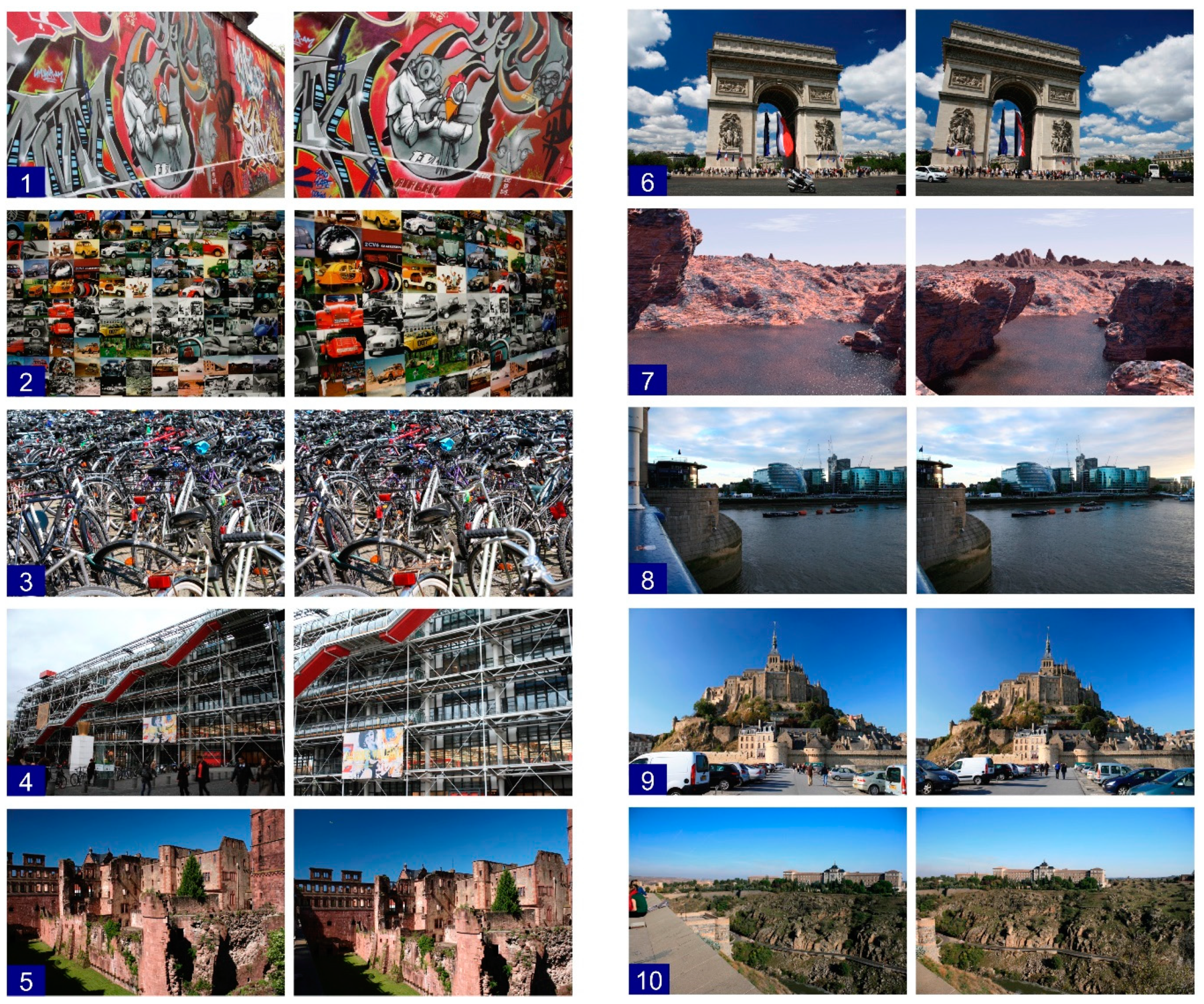
This set encompasses ten image pairs with a resolution of 1200 × 800 pixels. They are obtained by common geometric transformations, such as perspective, translation, rotation, and different degree scale (Figure 8). The set includes walls and landscapes in natural lighting settings exhibiting many regions of correspondence.
In Algorithm 1, the first step determines the k-sets of corresponding pairs. This process was carried out using the SURF algorithm [12], from which the best i-sets with the minimum projection error in accordance with the MLESAC estimator were selected. To properly evaluate the algorithm performance, 300 corresponding points in multiple locations inside each pair of images were selected. The accuracy of the algorithm at determining the correspondence upon the variation of the and the parameters were then assessed. For the latter, values were rounded. The results of the above-described analysis are presented below.
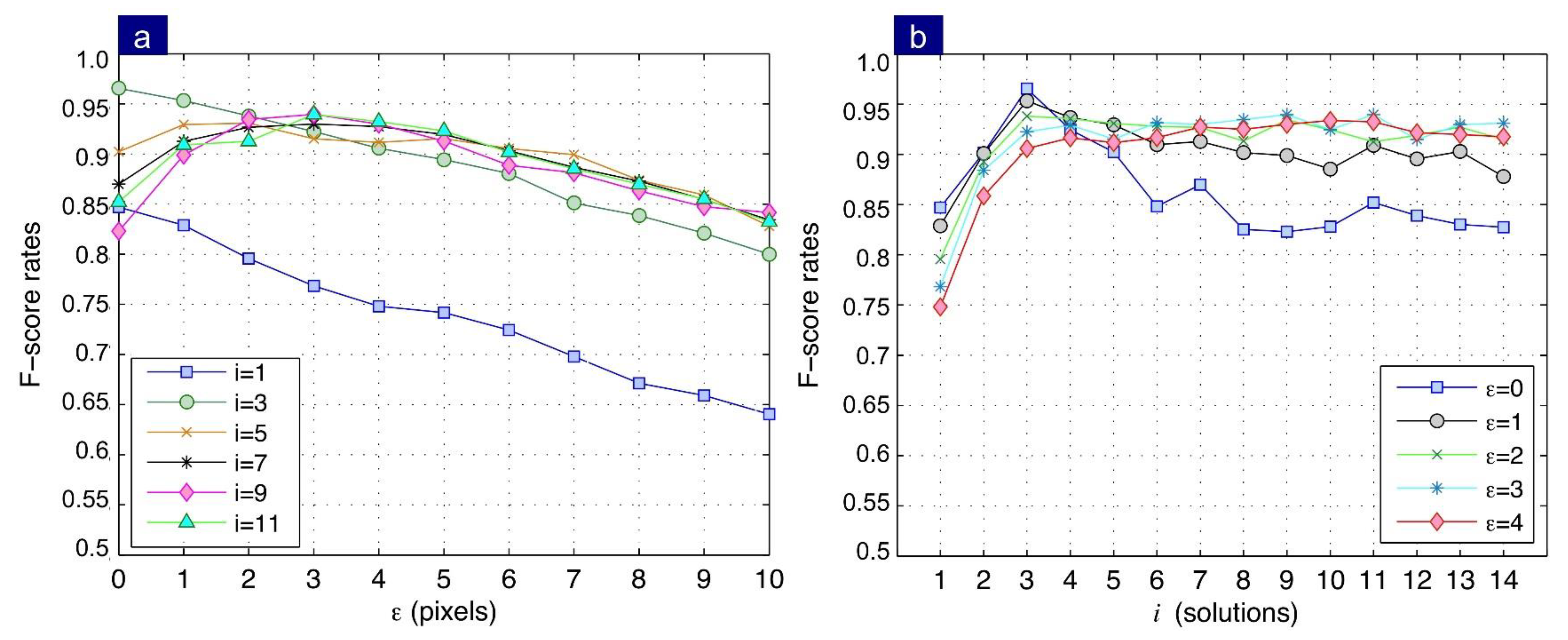
In the first case, the influence of parameter while keeping fixed was analyzed. Figure 9a shows that the best performance achieves an F-score = 0.97 at a discretized distance by intersecting three fundamental matrices, that is equal to 3. Note that, as increases, performance drops. This result is a clear indication that the method is particularly accurate, because there is a significant number of correspondences that have a low error, and the combination of these allows obtaining a corresponding point with high precision.
In the second case, the influence of parameter while keeping the number of solutions fixed was analyzed. Results show a maximum performance at . Conversely, an increase in this value determines the projection error’s growth, thus decreasing the method performance.
Remember that numerous correspondences are detected in the analyzed sequence despite the geometric transformations in them. Therefore, the results show the proposed model can use and estimate the perspective projection model in two sights with high precision with subpixel resolution. According to the performance shown in Figure 9b, after , it is evident that no improvements in the performance are obtained for .
4.2. Indoor Image Set
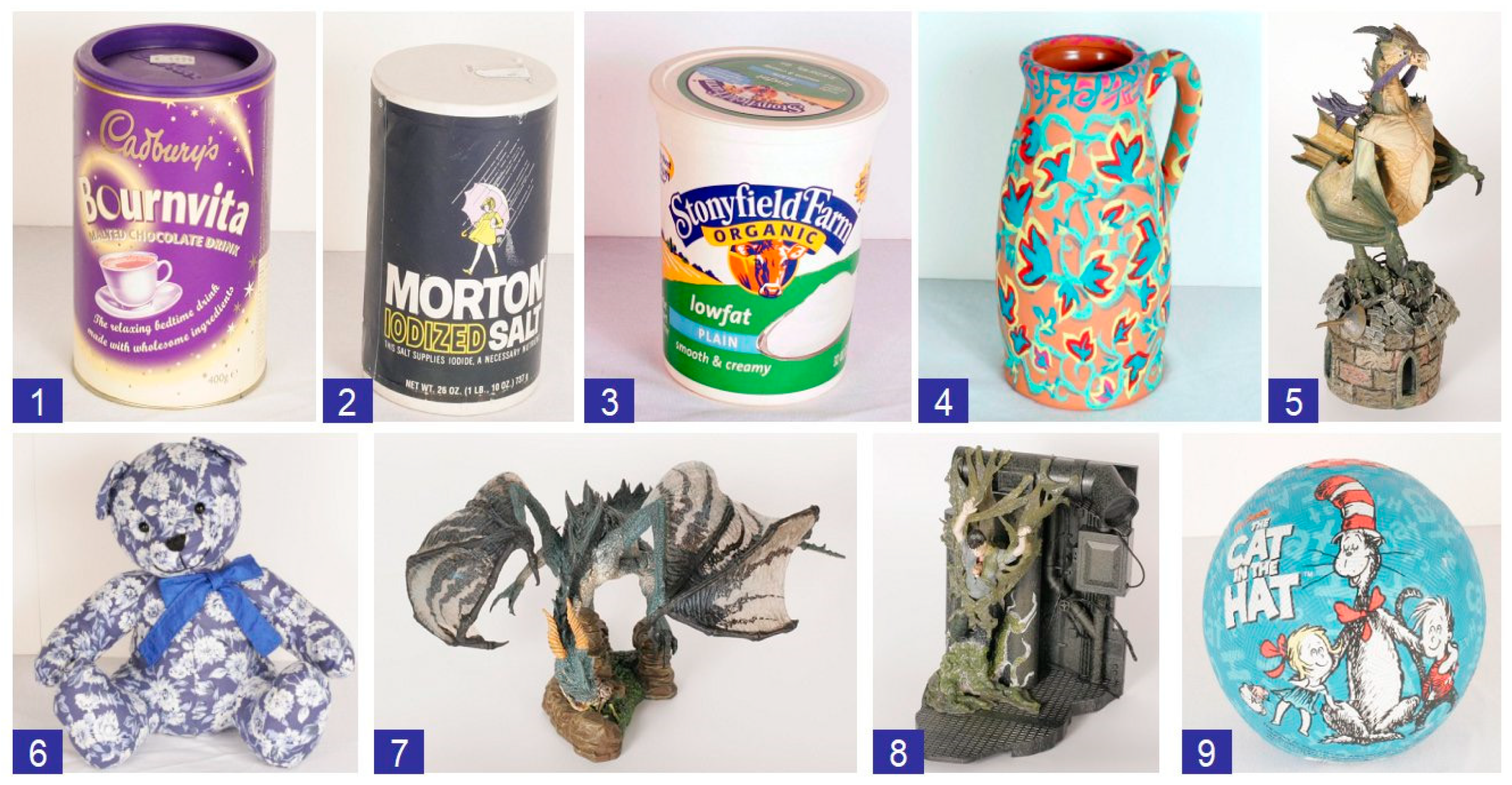
The second test considers a set of nine stereo sample images featured by 600 × 900 pixels resolution, generated in [46] (Figure 10). This set resulted by changing the points of view, rotating each object on its vertical axis. Therefore, the number of detected elemental correspondences is reduced, and also, these lasts are more closely distributed in each pair of pictures. As in the outdoor image set, 300 corresponding points in multiple locations in each image couple were detected using the SURF algorithm.
The same procedure was followed: the results for the variations of parameters and were determined. In the first case, the influence of parameter while keeping fixed was analyzed. Figure 11a shows that the method produces a maximum for ; however, from , the performance tends to stabilize considering a value . Figure 11b indicates that using a single fundamental matrix () causes low performance (60%). In contrast, using multiple solutions, an improvement in performance from 20% to 25% is achieved.
4.3. Industrial Image Set
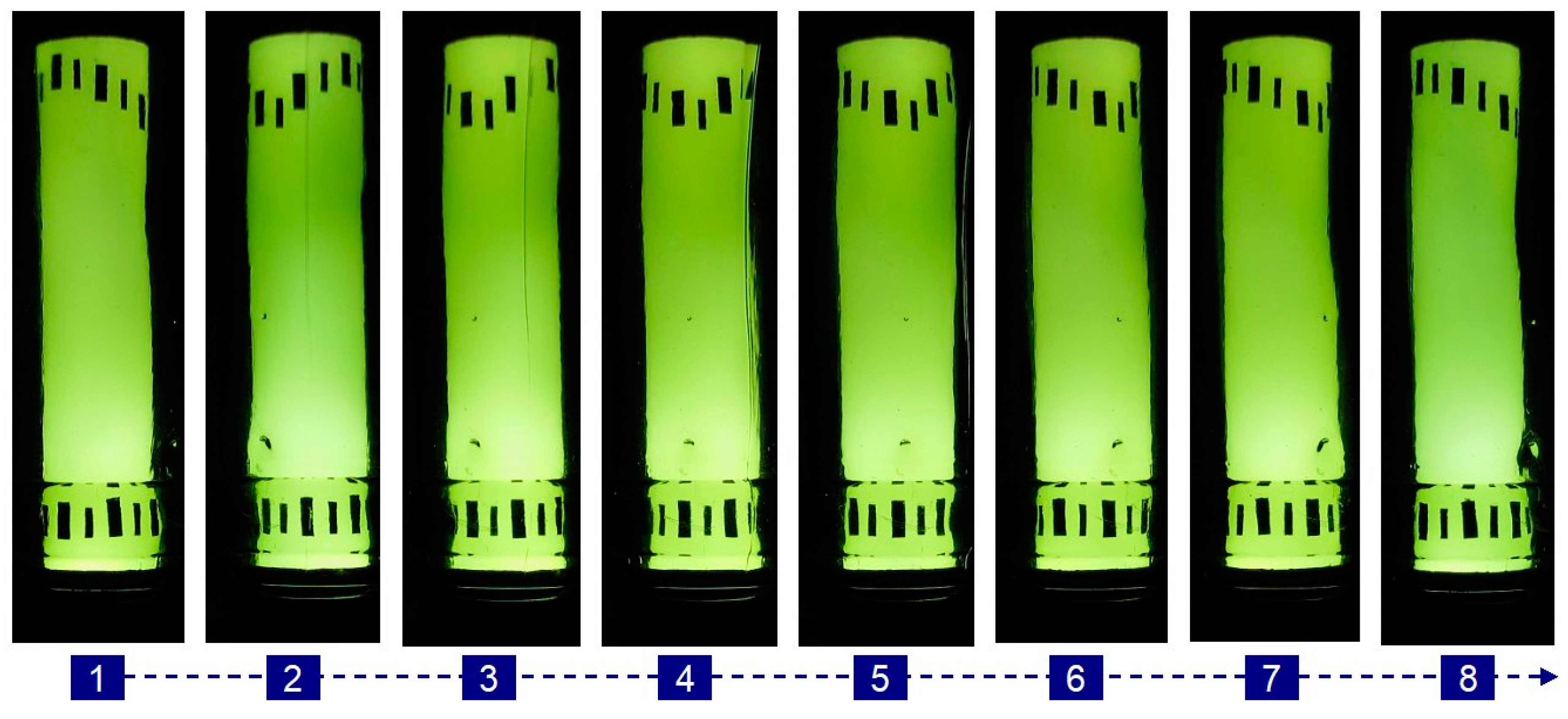
The third and last set includes 120 sequences of faulty bottlenecks images with low SNR generated in [47] (Figure 12). Each sequence comprises three pictures with an axial angle of rotation α = 15°. From the captured images, 1000 × 250 pixels sub-images were extracted. The elemental correspondence was detected employing markers outside the object in accordance with the object’s motion. Point-to-point correspondence detection aimed to identify the trajectory of multiple errors in the sequence, for determining the bottle quality in an inspection process featured by multiple views.
4.3.1. Evaluation According to the Number of Partial Solutions
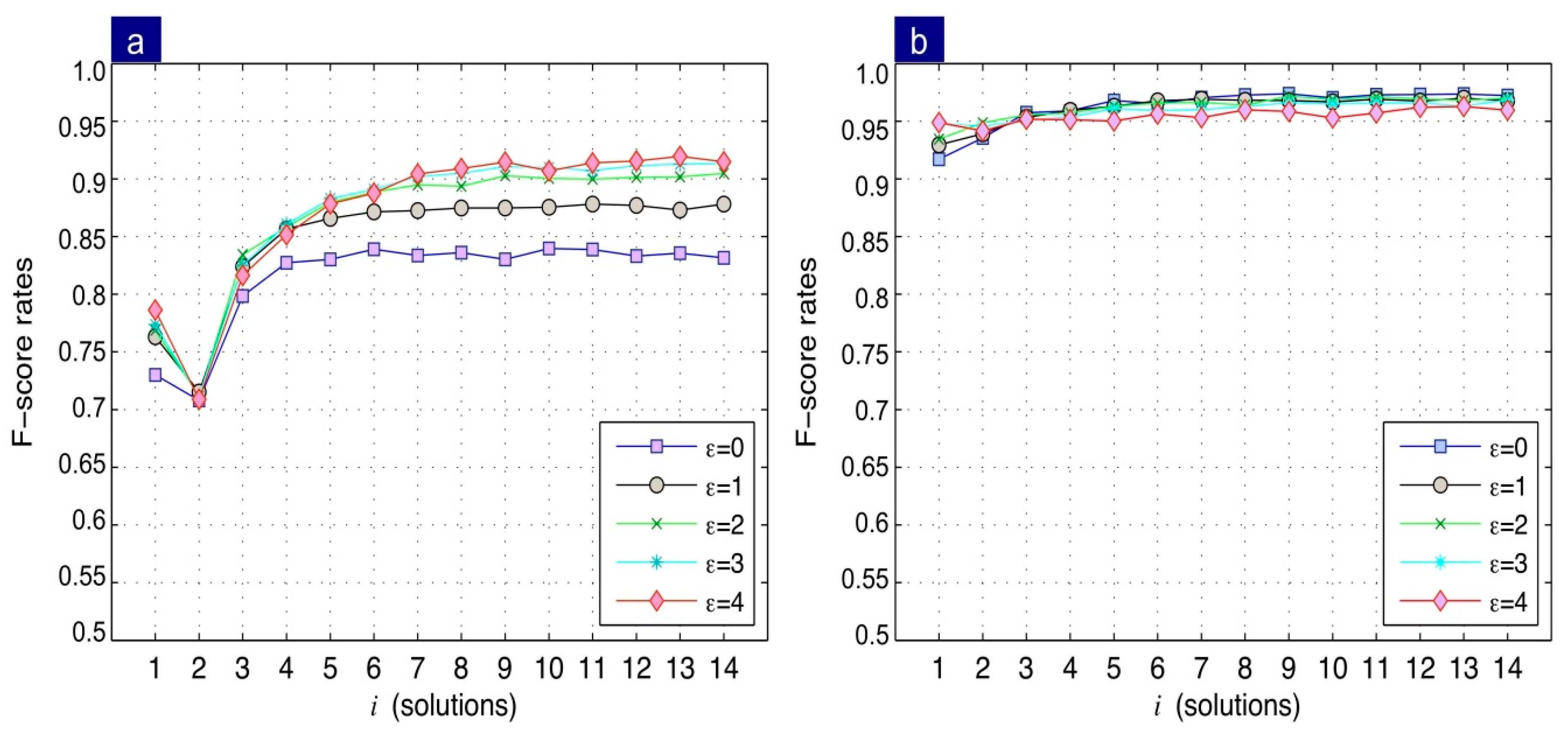
Now, we consider the results of two and three views separately, shown in Figure 13a and Figure 13b, respectively.
- (1)
- Two views: Results indicate that the F-score directly depends on the increase of parameter , becoming stable at . Regarding the influence of parameter on the F-score, an improvement of performance is achieved as the distance between the epipolar line and the corresponding point increases. Further, note that the performance stabilizes after . These results imply that a better performance can be obtained when the combination is used and when the distance to the corresponding point is .
- (2)
- Three views: Unlike the two-view case, the best performance was obtained when a discretized distance was employed. Similarly, to the two views, the combination is repeated. Results indicate that at a trifocal correspondence with an F-score = 0.97 is obtained. Note that the method performance decreases as the parameter increases. This behaviour is in antithesis with that obtained in the two-view case. This is because the method in three views does not use the intersection of lines, but the reprojection of a coordinate in a third view. For this reason, the greater the distance , the performance decreases, since the precision of the reprojection method is high.
4.3.2. Evaluation According to the Re-Projection Distance
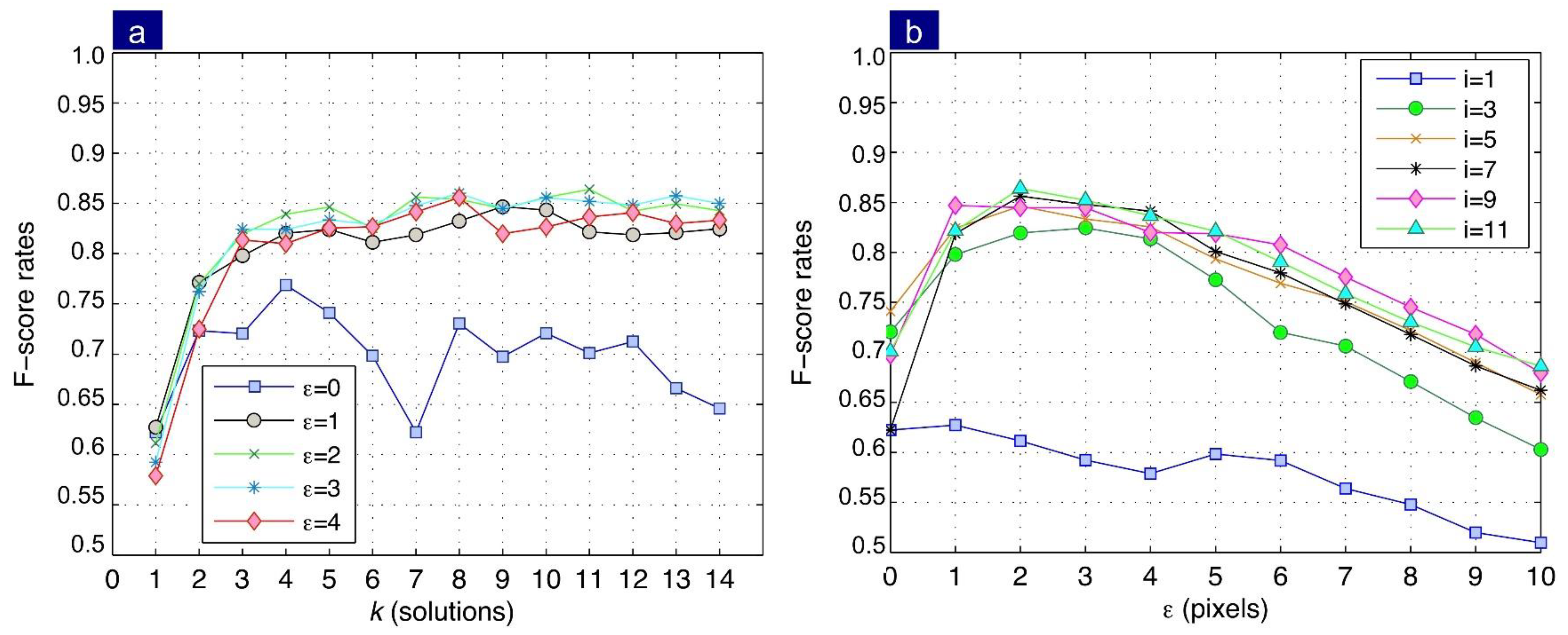
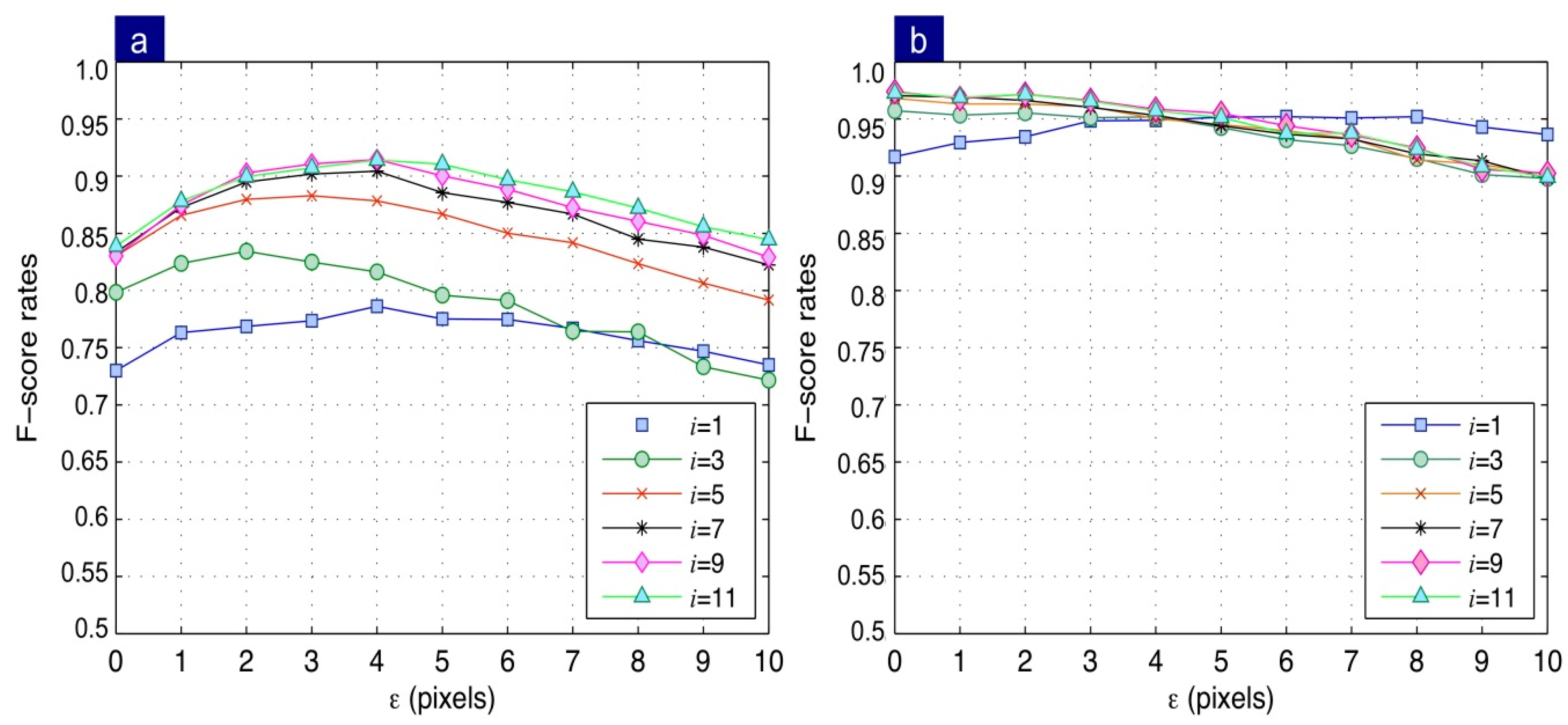
In the previous evaluation, parameter was varied to determine its influence on the performance of the system of correspondences. In this case, the influence of the distance while keeping parameter fixed was evaluated. Due to the significant number of resulting curves, Figure 14 shows only the odd numbers of parameter . Results for two (Figure 14a) and three views (Figure 14b) are summarized as follows:
- (1)
- Two views: the obtained results agree with the discussion above reported concerning the number of intermediate solutions. For , i.e., only one epipolar line is used, a maximum F-score of 0.78 is obtained for a distance of four pixels. For and , performance increases to an F-score = 0.87. Taking and using combination, allows a performance increase to an F-score = 0.87. Finally, for nine combinations, the maximum performance, corresponding to an F-score = 0.91, is obtained.
- (2)
- Three views: a significant difference between using single trifocal tensor respect to the multiple trifocal tensors is observed. For instance, considering a single trifocal tensor (), the maximum performance is achieved for a distance of six pixels resulting in an F score equal to 0.95. Conversely, when using nine combinations, an F-score = 0.97 at a discretized distance is obtained. The latter result indicates the validity of the proposed method by using a combination of multiple intermediate solutions. The more significant false alarms number is ascribable to the discrepancy of the performance between two and three-sights detection. Two views detection achieves a greater false alarms number compared to the three views detection. This occurs because, in two views, the process requires the intersection of multiple epipolar lines. In the case of three views, a reprojection is carried out, which uses more information from the control points, and thus its estimation error is lower.
4.3.3. Results Discussion and Performance Comparison of the Developed Point-Matching Methods
A popular way to find correspondences is utilizing similarity over a set of feature descriptors. The NNDR criterion [13] is commonly used for such purpose. The idea behind NNDR is that each invariant descriptor can be found in other perspectives with high probability. Its main limitation is that it can filter out many potential matches; some of them correct matches. For most applications, this limitation is acceptable. However, to fairly compare our algorithm with NNDR, we evaluated the universe of matches filtered out versus the set of real ones.
Table 1 compares the performances obtained between NNDR, and the proposed BIGC and TRIGC. Note that NNDR achieves the lowest performance as it filters out many correct matches. Our proposed BIGC and TRIGC methods outperform NNDR using a combination of feature descriptors and geometrical analysis.
It can be therefore concluded that the use of multiple hypotheses improves the original matching criterion reducing the set of false alarms. As we mentioned in the previous discussion, the advantage of our proposal lies in the use of multiple partial solutions, which in combination allow to obtain a significant improvement in the correspondence of multiple points. This is especially reflected in images of the outdoor and industrial scenarios, obtaining 97% and 91% in a sequence of two images, respectively, by means of developed BIGC algorithm (Table 1). In the case of three images, the method uses as input the matching between pairs of images. Given that high performance obtained with the BIGC algorithm, we have obtained an F-score equals to 97%.
Figure 15 shows the method’s best performance using the optimum value of as function of the parameter . Note that from five combinations () using three views, zero pixels remain the optimal distance. This plot’s results agree with those previously presented; both for two and three views, the best performance is reached for .
5. Conclusions
This paper has reported a new method for detecting point matching based on the intersection of different geometric hypothesized solutions in two and three perspectives. A major contribution of the proposal is that, for each perspective projection model, it determines the real distance from the corresponding point using the MLESAC estimator, weighting the error associated to each intermediate solution.
The main novelty of the proposed approach is the geometric methodology to determine the point-to-point correspondence regardless of (1) the viewpoint differences of the objects present in the images and (2) the geometric/photometric transformations in them. The proposed algorithms are named Bifocal Geometric Correspondence BIGC and Trifocal Geometric Correspondence TRIGC for the correspondence detection in two and three sights, respectively.
The developed method has experimentally demonstrated the feasibility of using fundamental matrices to find corresponding points in two views. For points that can be occluded in subsequent views, the method shows that their positions remain valid. The method suggests that the proper use of multiple random solutions improves the correspondence performance. Taking the set of points of a previous correspondence, the method calculates fundamental matrices Fi and trifocal tensors Ti to maximize the correspondences in specific regions of each image.
For experimental validation, three sets of images were used: indoor, outdoor, and industrial images. For outdoor and indoor images, we have used a correspondence through the SURF’s invariant features with the purpose of obtaining multiple geometric solutions in two views [10]. The experimental results obtained with these sets have demonstrated that the BIGC algorithm allowed to determine the point-to-point correspondence very precisely:
- (1)
- For outdoor images, with a performance F-score = 97% in stereo images and at a discretized distance pixel.
- (2)
- For indoor images, with a performance F-score = 87% with by using a distance of . The lower F-score in indoor images is partially resulting from the lower dispersion of correspondences in the pairs of images.
For the industrial images, the base correspondence was established according to the relation of external markers that comply properly with the object motion. The TRIGC algorithm exhibited the best performance with an F-score = 97% at a discretized distance of pixel in a sequence of three views implying that the correspondence has a subpixel resolution.
For all the images considered in this scientific article, it was demonstrated that the point-to-point correspondence could be obtained through a multiple geometric relation between two or three views, regardless of the base method of correspondence used.
An interesting feature of our proposal is that it can be used in sequences of images exhibiting low SNR. Traditional invariant algorithms do not achieve good performance in these cases due to the appearance of many false alarms. Our method can actually solve this problem thanks to its geometric background, as widely illustrated in the set of industrial images.
Author Contributions
Conceptualization, M.C. and D.M.; methodology, M.C. and A.C.; software, M.C and R.D.F.; validation, M.C. and D.M.; data curation, R.V. and P.V.; writing—original draft preparation, M.C and P.V.; writing—review and editing, P.V., R.D.F. and R.V. All authors have read and agreed to the published version of the manuscript.
Funding
This research received no external funding.
Informed Consent Statement
Informed consent was obtained from all subjects involved in the study.
Data Availability Statement
Data of our study are available upon request
Conflicts of Interest
The authors declare no conflict of interest.
References
- Mindru, F.; Tuytelaars, T.; Gool, L.V.; Moons, T. Moment invariants for recognition under changing viewpoint and illumination. Comput. Vis. Image Underst. 2004, 94, 3–27. [Google Scholar] [CrossRef]
- Pissaloux, E.E.; Maybank, S.; Velázquez, R. On Image Matching and Feature Tracking for Embedded Systems: A State-of-the-Art. In Advances in Heuristic Signal Processing and Applications; Chatterjee, A., Nobahari, H., Siarry, P., Eds.; Springer: Berlin/Heidelberg, Germany, 2013; pp. 357–380. ISBN 978-3-642-37879-9. [Google Scholar]
- Bhat, P.; Zheng, K.C.; Snavely, N.; Agarwala, A.; Agrawala, M.; Cohen, M.F.; Curless, B. Piecewise Image Registration in the Presence of Multiple Large Motions. In Proceedings of the IEEE Conference on Computer Vision and Pattern Recognition, New York, NY, USA, 17–22 June 2006; IEEE: New York, NY, USA, 2006; Volume 2, pp. 2491–2497. [Google Scholar]
- López-Martínez, A.; Cuevas, F.J. Multiple View Relations Using the Teaching and Learning-Based Optimization Algorithm. Computers 2020, 9, 101. [Google Scholar] [CrossRef]
- Kadir, T.; Zisserman, A.; Brady, M. An Affine Invariant Salient Region Detector. In Lecture Notes in Computer Science; Springer: Berlin/Heidelberg, Germany, 2004; Volume 1, pp. 228–241. [Google Scholar] [CrossRef]
- Matas, J.; Chum, O.; Urban, M.; Pajdla, T. Robust wide baseline stereo from maximally stable extremal regions. Image Vis. Comp. 2004, 22, 761–767. [Google Scholar] [CrossRef]
- Mikolajczyk, K.; Schmid, C. Scale & Affine Invariant Interest Point Detectors. Int. J. Comp. Vis. 2004, 60, 63–86. [Google Scholar] [CrossRef]
- Tuytelaars, T.; Mikolajczyk, K. Local Invariant Feature Detectors: A Survey. Found. Trends Comput. Graph. Vis. 2008, 3, 177–280. [Google Scholar] [CrossRef] [Green Version]
- Pizarro, L.; Mery, D.; Delpiano, R.; Carrasco, M. Robust automated multiple view inspection. Pattern Anal. Appl. 2008, 11, 21–32. [Google Scholar] [CrossRef] [Green Version]
- Reddy, N.D.; Vo, M.; Narasimhan, S.G. Occlusion-Net: 2D/3D Occluded Keypoint Localization Using Graph Networks. In Proceedings of the 2019 IEEE/CVF Conference on Computer Vision and Pattern Recognition (CVPR), Long Beach, CA, USA, 15–20 June 2019; pp. 7318–7327. [Google Scholar]
- Carrasco, M.; Mery, D. Bifocal Matching using Multiple Geometrical Solutions. In Advances in Image and Video Technology—5th Pacific Rim Symposium, PSIVT 2011; Spinger: Berlin/Heidelberg, Germany, 2011; Volume 7088, pp. 192–203. [Google Scholar]
- Bay, H.; Ess, A.; Tuytelaars, T.; Gool, L.V. SURF: Speeded up robust features. Comput. Vis. Image Underst. 2008, 110, 346–359. [Google Scholar] [CrossRef]
- Lowe, D.G. Distinctive Image Features from Scale-Invariant Keypoints. Int. J. Comput. Vis. 2004, 60, 91–110. [Google Scholar] [CrossRef]
- Bosch, A.; Zisserman, A.; Munoz, X. Representing shape with a spatial pyramid kernel. In Proceedings of the 6th ACM International Conference on Image and Video Retrieval (CIVR), Amsterdam, The Netherlands, 9–11 July 2007; pp. 401–408. [Google Scholar]
- Caspi, Y.; Irani, M. A step towards sequence-to-sequence alignment. In Proceedings of the IEEE Conference on Computer Vision and Pattern Recognition (CVPR), Hilton Head Island, South Carolina, 13–15 June 2000; Volume 2, pp. 682–689. [Google Scholar]
- Fitzgibbon, A. Robust registration of 2D and 3D point sets. Image Vis. Comput. 2003, 21, 1145–1153. [Google Scholar] [CrossRef]
- Chen, H.; Aldea, E.; Le Hegarat-Mascle, S. Integrating Visual and Geometric Consistency for Pose Estimation. In Proceedings of the 2019 16th International Conference on Machine Vision Applications (MVA), Tokyo, Japan, 27–31 May 2019; pp. 1–5. [Google Scholar]
- Oskarsson, M. Two-View Orthographic Epipolar Geometry: Minimal and Optimal Solvers. J. Math. Imaging Vis. 2018, 60, 163–173. [Google Scholar] [CrossRef] [Green Version]
- Vidal, R.; Ma, Y.; Soatto, S.; Sastry, S. Two-view multibody structure from motion. Int. J. Comput. Vis. 2006, 68, 7–25. [Google Scholar] [CrossRef] [Green Version]
- Mohamed, A.; Culverhouse, P.; Cangelosi, A.; Yang, C. Active stereo platform: Online epipolar geometry update. J. Image Video Proc. 2018, 2018, 54. [Google Scholar] [CrossRef]
- Kanberoglu, B.; Das, D.; Nair, P.; Turaga, P.; Frakes, D. An Optical Flow-Based Approach for Minimally Divergent Velocimetry Data Interpolation. Int. J. Biomed. Imaging 2019, 2019, 9435163. [Google Scholar] [CrossRef] [PubMed] [Green Version]
- Dudek, R.; Cuenca, C.; Quintana, F. An Automatic Optical Flow Based Method for the Detection and Restoration of Non-repetitive Damaged Zones in Image Sequences. In Visual Informatics: Bridging Research and Practice; Badioze Zaman, H., Robinson, P., Petrou, M., Olivier, P., Schröder, H., Shih, T.K., Eds.; Lecture Notes in Computer Science; Springer: Berlin/Heidelberg, Germany, 2009; Volume 5857, pp. 800–810. ISBN 978-3-642-05035-0. [Google Scholar]
- Sur, F.; Noury, N.; Berger, M.-O. An A Contrario Model for Matching Interest Points under Geometric and Photometric Constraints. SIAM J. Imaging Sci. 2013, 6, 1956–1978. [Google Scholar] [CrossRef]
- Scharstein, D.; Szeliski, R. A Taxonomy and Evaluation of Dense Two-Frame Stereo Correspondence Algorithms. Int. J. Comput. Vis. 2002, 47, 7–42. [Google Scholar] [CrossRef]
- Barron, J.L.; Fleet, D.J.; Beauchemin, S.S. Performance of Optical Flow Techniques. Int. J. Comput. Vis. 1994, 12, 43–77. [Google Scholar] [CrossRef]
- Hartley, R.; Zisserman, A. Multiple View Geometry in Computer Vision, 2nd ed.; Cambridge University Press: Cambridge, UK, 2000; ISBN 0-521-54051-8. [Google Scholar]
- Peng, L.; Zhang, Y.; Zhou, H.; Lu, T. A Robust Method for Estimating Image Geometry with Local Structure Constraint. IEEE Access 2018, 6, 20734–20747. [Google Scholar] [CrossRef]
- Chen, Z.; Wu, C.; Shen, P.; Liu, Y.; Quan, L. A robust algorithhm to estimate the fundamental matrix. Pattern Recognit. Lett. 2000, 21, 851–861. [Google Scholar] [CrossRef]
- Bartoli, A.; Sturm, P. Nonlinear estimation of the fundamental matrix with minimal parameters. IEEE Trans. Pattern Anal. Mach. Intell. 2004, 26, 426–432. [Google Scholar] [CrossRef] [Green Version]
- Mendes Júnior, P.R.; de Souza, R.M.; de Werneck, R.O.; Stein, B.V.; Pazinato, D.V.; de Almeida, W.R.; Penatti, O.A.B.; da Torres, R.S.; Rocha, A. Nearest neighbors distance ratio open-set classifier. Mach. Learn. 2017, 106, 359–386. [Google Scholar] [CrossRef] [Green Version]
- Dominguez-Morales, M.; Domínguez-Morales, J.P.; Jiménez-Fernández, Á.; Linares-Barranco, A.; Jiménez-Moreno, G. Stereo Matching in Address-Event-Representation (AER) Bio-Inspired Binocular Systems in a Field-Programmable Gate Array (FPGA). Electronics 2019, 8, 410. [Google Scholar] [CrossRef] [Green Version]
- Shao, M.; Hu, M. Parallel feature based calibration method for a trinocular vision sensor. Opt. Express 2020, 28, 20573. [Google Scholar] [CrossRef] [PubMed]
- Shashua, A. Algebraic functions for recognition. IEEE Trans. Pattern Anal. Mach. Intell. 1995, 17, 779–789. [Google Scholar] [CrossRef]
- Fischler, M.A.; Bolles, R.C. Random sample consensus: A paradigm for model fitting with applications to image analysis and automated cartography. Commun. ACM 1981, 24, 381–395. [Google Scholar] [CrossRef]
- Torr, P.H.S.; Zisserman, A. MLESAC: A New Robust Estimator with Application to Estimating Image Geometry. Comput. Vis. Image Underst. 2000, 78, 138–156. [Google Scholar] [CrossRef] [Green Version]
- Li, R.; Sun, J.; Gong, D.; Zhu, Y.; Li, H.; Zhang, Y. ARSAC: Efficient model estimation via adaptively ranked sample consensus. Neurocomputing 2019, 328, 88–96. [Google Scholar] [CrossRef]
- Wong, H.S.; Chin, T.-J.; Yu, J.; Suter, D. A simultaneous sample-and-filter strategy for robust multi-structure model fitting. Comput. Vis. Image Underst. 2013, 117, 1755–1769. [Google Scholar] [CrossRef]
- Tordoff, B.J.; Murray, D.W. Guided-MLESAC: Faster image transform estimation by using matching priors. IEEE Trans. Pattern Anal. Mach. Intell. 2005, 27, 1523–1535. [Google Scholar] [CrossRef] [Green Version]
- Wöhler, C. 3D Computer Vision; X.media.publishing; Springer: London, UK, 2013; ISBN 978-1-4471-4149-5. [Google Scholar]
- Pellicanò, N.; Aldea, E.; Le Hégarat-Mascle, S. Wide baseline pose estimation from video with a density-based uncertainty model. Mach. Vis. Appl. 2019, 30, 1041–1059. [Google Scholar] [CrossRef] [Green Version]
- Torr, P.H.S. Bayesian Model Estimation and Selection for Epipolar Geometry and Generic Manifold Fitting. Int. J. Comput. Vis. 2002, 50, 35–61. [Google Scholar] [CrossRef]
- Arrigoni, F.; Magri, L.; Pajdla, T. On the Usage of the Trifocal Tensor in Motion Segmentation. In Computer Vision—ECCV 2020; Vedaldi, A., Bischof, H., Brox, T., Frahm, J.-M., Eds.; Lecture Notes in Computer Science; Springer International Publishing: Cham, Switzerland, 2020; Volume 12365, pp. 514–530. ISBN 978-3-030-58564-8. [Google Scholar]
- Viwatwongkasem, C. EM Algorithm for Normal Mixture Likelihoods. In Proceedings of the 2018 International Electrical Engineering Congress (iEECON), Krabi, Thailand, 7–9 March 2018; pp. 1–4. [Google Scholar]
- Li, B. Stereo Imaging with Uncalibrated Camera. In Advances in Visual Computing; Lecture Notes in Computer Science; Springer: Berlin/Heidelberg, Germany, 2006; Volume 4291, pp. 112–121. ISBN 978-3-540-48628-2. [Google Scholar]
- Gaetani, F.; Primiceri, P.; Antonio Zappatore, G.; Visconti, P. Hardware design and software development of a motion control and driving system for transradial prosthesis based on a wireless myoelectric armband. IET Sci. Meas. Technol. 2019, 13, 354–362. [Google Scholar] [CrossRef]
- Akash Kushal, J.P. Modeling 3D objects from stereo views and recognizing them in photographs. In Lecture Notes in Computer Science; Springer: Berlin/Heidelberg, Germany, 2006; Volume 3952, pp. 563–574. [Google Scholar]
- Carrasco, M.; Pizarro, L.; Mery, D. Image Acquisition and Automated Inspection of Wine Bottlenecks by Tracking in Multiple Views. In Proceedings of the 8th WSEAS International Conference on Signal Processing, Computational Geometry and Artificial Vision (ISCGAV’08), Rhodes, Greece, 20–22 August 2008; pp. 82–89. [Google Scholar]
- Calabrese, B.; Velázquez, R.; Del-Valle-Soto, C.; de Fazio, R.; Giannoccaro, N.I.; Visconti, P. Solar-Powered Deep Learning-Based Recognition System of Daily Used Objects and Human Faces for Assistance of the Visually Impaired. Energies 2020, 13, 6104. [Google Scholar] [CrossRef]
- Olson, D.; Delen, D. Advanced Data Mining Techniques; Springer: Berlin/Heidelberg, Germany, 2008; ISBN 978-3-540-76916-3. [Google Scholar]
- Carrasco, M.; Álvarez, F.; Velázquez, R.; Concha, J.; Pérez-Cotapos, F. Brush-Holder Integrated Load Sensor Prototype for SAG Grinding Mill Motor. Electronics 2019, 8, 1227. [Google Scholar] [CrossRef] [Green Version]
- Visconti, P.; Gaetani, F.; Zappatore, G.A.; Primiceri, P. Technical features and functionalities of MYO armband: An overview on related literature and advanced applications of myoelectric bracelets mainly focused on arm prostheses. Int. J. Smart Sens. Intell. Syst. 2018, 11, 1–25. [Google Scholar] [CrossRef] [Green Version]
Figure 1.
The point-matching problem in multiple views: determined a point r in I1, then we have to find the correspondences in I2 and I3.
Figure 1.
The point-matching problem in multiple views: determined a point r in I1, then we have to find the correspondences in I2 and I3.

Figure 2.
The epipolar geometry of an object in the 3D space and its projections in 2D planes.

Figure 3.
Three view-based epipolar geometry of an object in the 3D space.

Figure 4.
The k subsets of epipolar lines from multiple optical centers.

Figure 5.
Illustration of the set of correspondences creating the new epipolar lines: , , and . For simplicity, only four corresponding points are shown (the method actually uses seven).
Figure 5.
Illustration of the set of correspondences creating the new epipolar lines: , , and . For simplicity, only four corresponding points are shown (the method actually uses seven).

Figure 6.
Point-correspondence and detection of wrong matches using the multiple geometric correspondence (MGC) filter.
Figure 6.
Point-correspondence and detection of wrong matches using the multiple geometric correspondence (MGC) filter.

Figure 7.
The trifocal re-projections of the sets of independent correspondences in a third view.

Figure 8.
The outdoor image set.

Figure 9.
Average performance obtained in the outdoor image set: (a) The effect of in the method’s performance. (b) Influence of parameter i on performance as a function of .
Figure 9.
Average performance obtained in the outdoor image set: (a) The effect of in the method’s performance. (b) Influence of parameter i on performance as a function of .

Figure 10.
The indoor image set.

Figure 11.
Average performance obtained in the indoor image set: (a) Influence of parameter i on performance as a function of . (b) The effect of in the method performance as a function of parameter i.
Figure 11.
Average performance obtained in the indoor image set: (a) Influence of parameter i on performance as a function of . (b) The effect of in the method performance as a function of parameter i.

Figure 12.
The industrial image set.

Figure 13.
Performance of the proposed method as a function of the i and different values of : (a) two and (b) three views.
Figure 13.
Performance of the proposed method as a function of the i and different values of : (a) two and (b) three views.

Figure 14.
Influence of on performance for a different number of solutions i: (a) two and (b) three views.
Figure 14.
Influence of on performance for a different number of solutions i: (a) two and (b) three views.

Figure 15.
The best performance as a function of the number of solutions i.


Table 1.
Performance comparison between NNDR, BIGC, and TRIGC methods: real matching set.
| Method | Indoor [%] | Outdoor [%] | Industrial [%] |
|---|---|---|---|
| NNDR | 77 | 75 | 82 |
| BIGC | 87 | 97 | 91 |
| TRIGC | N/A | N/A | 97 |
Publisher’s Note: MDPI stays neutral with regard to jurisdictional claims in published maps and institutional affiliations. |
© 2021 by the authors. Licensee MDPI, Basel, Switzerland. This article is an open access article distributed under the terms and conditions of the Creative Commons Attribution (CC BY) license (http://creativecommons.org/licenses/by/4.0/).
Share and Cite
MDPI and ACS Style
Carrasco, M.; Mery, D.; Concha, A.; Velázquez, R.; De Fazio, R.; Visconti, P. An Efficient Point-Matching Method Based on Multiple Geometrical Hypotheses. Electronics 2021, 10, 246. https://doi.org/10.3390/electronics10030246
AMA Style
Carrasco M, Mery D, Concha A, Velázquez R, De Fazio R, Visconti P. An Efficient Point-Matching Method Based on Multiple Geometrical Hypotheses. Electronics. 2021; 10(3):246. https://doi.org/10.3390/electronics10030246
Chicago/Turabian StyleCarrasco, Miguel, Domingo Mery, Andrés Concha, Ramiro Velázquez, Roberto De Fazio, and Paolo Visconti. 2021. "An Efficient Point-Matching Method Based on Multiple Geometrical Hypotheses" Electronics 10, no. 3: 246. https://doi.org/10.3390/electronics10030246
Note that from the first issue of 2016, this journal uses article numbers instead of page numbers. See further details here.