Foliar Moisture Content from the Spectral Signature for Wildfire Risk Assessments in Valparaíso-Chile
by
 , and
, and
Juan Villacrés
1,†,‡ ,
,
Tito Arevalo-Ramirez
1,†,‡,
Andrés Fuentes
2,†,‡,
Pedro Reszka
3,‡ and
Fernando Auat Cheein
1,*,†,‡ 1
Department of Electronic Engineering, Universidad Técnica Federico Santa María, Valparaiso 2390123, Chile
2
Department of Industrial Engineering, Universidad Técnica Federico Santa María, Valparaiso 2390123, Chile
3
Faculty of Engineering and Sciences, Universidad Adolfo Ibáñez, Santiago 7941169, Chile
*
Author to whom correspondence should be addressed.
†
Current address: Av. España 1680, Valparaiso 2390123, Chile.
‡
These authors contributed equally to this work.
Sensors 2019, 19(24), 5475; https://doi.org/10.3390/s19245475
Submission received: 22 September 2019
/
Revised: 18 October 2019
/
Accepted: 22 October 2019
/
Published: 12 December 2019
(This article belongs to the Section Remote Sensors)
Abstract
:Fuel moisture content (FMC) proved to be one of the most relevant parameters for controlling fire behavior and risk, particularly at the wildland-urban interface (WUI). Data relating FMC to spectral indexes for different species are an important requirement identified by the wildfire safety community. In Valparaíso, the WUI is mainly composed of Eucalyptus Globulus and Pinus Radiata—commonly found in Mediterranean WUI areas—which represent the 97.51% of the forests plantation inventory. In this work we study the spectral signature of these species under different levels of FMC. In particular, we analyze the behavior of the spectral reflectance per each species at five dehydration stages, obtaining eighteen spectral indexes related to water content and, for Eucalyptus Globulus, the area of each leave—associated with the water content—is also computed. As the main outcome of this research, we provide a validated linear regression model associated with each spectral index and the fuel moisture content and moisture loss, per each species studied.
1. Introduction
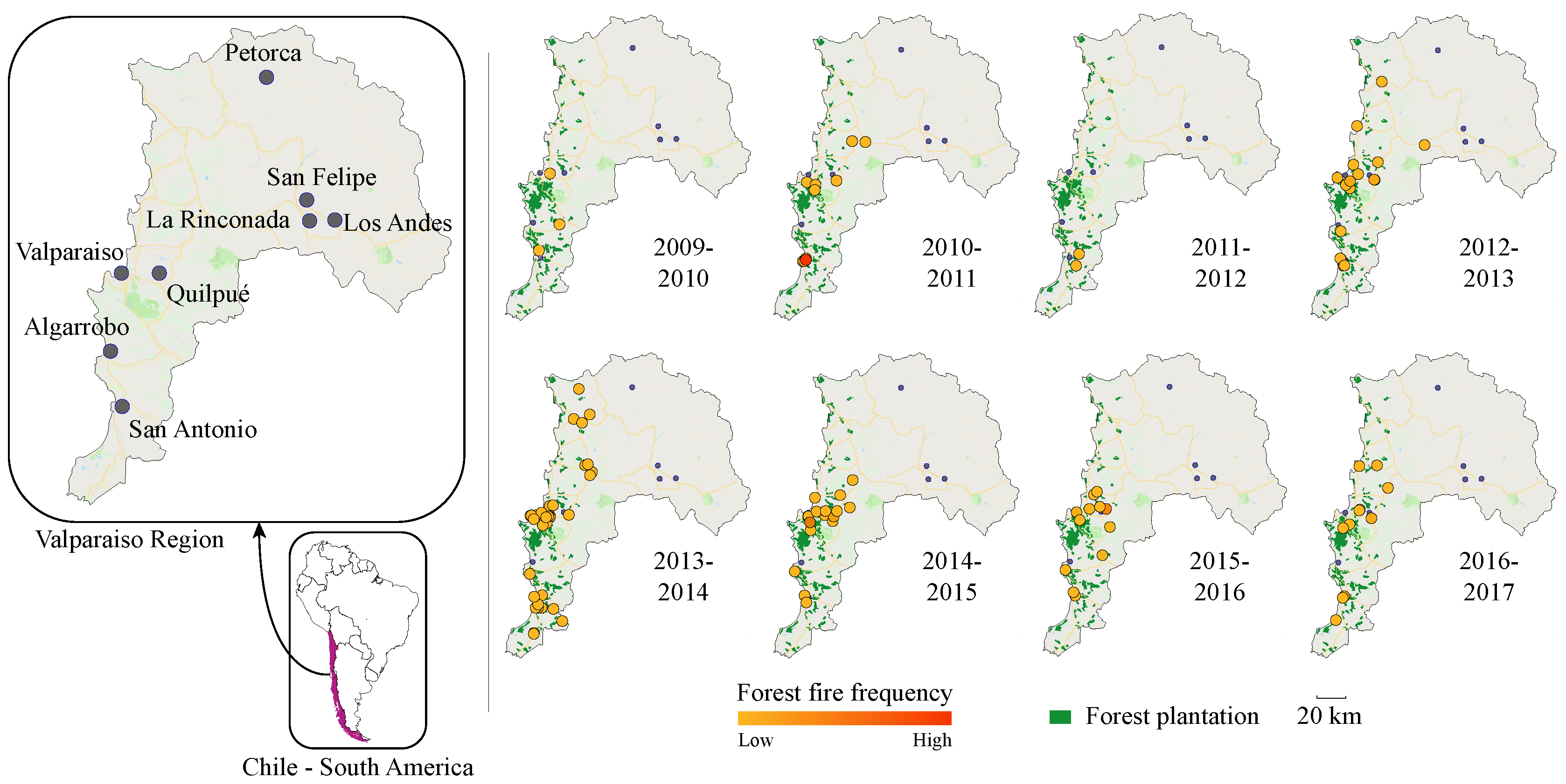
The latest wildfire seasons in Chile have caused significant human, ecological and economic losses in cities, in the forestry industry and in protected areas. Recently, the fires in early 2017 caused 11 fatalities, burned more than 550,000 ha and destroyed more than 1000 houses [1]. In particular, Valparaíso—a central region in Chile—has suffered the greatest losses from wildfires and represents the most challenging scenario for wildfire prevention, detection, and response, due to its topographical and urban social features [2]. According to Chile’s Forest Service (CONAF), from 2003 to 2018, 12,868 recorded wildfires burned 121,328.81 ha in Valparaiso [3]. The prone of Valparaíso to wildfires is given by the introduction of flammable species—i.e., Eucalyptus Globulus, Pinus Radiata—[3,4], both species represent the of the forest plantation [5]. Moreover, approximately 90% of such wildfires have been related to anthropogenic activities including transit of vehicles or aircraft, recreational activities, power line failures and arson attacks [6]. The sequence of maps presented in Figure 1 is a timeline of forest fire frequency in Valparaíso. Such figure offers a spatial visualization of areas majority affected [7]. Thus, given the susceptibility of Valparaíso to wildfires, it becomes crucial to allocate the areas with a higher risk for an adequate forest and wildland–urban interfaces (WUI) management.
Risk-based tools for decision making to manage forests and the WUI are cost-effective solutions to allocate resources in areas with higher risks [8,9]. However, their use requires an adequate wildfire modeling [10]. Such modeling needs of a reliable knowledge of the processes occurring in the solid and gaseous phases during the combustion of wildland fuels. Their ignition is an outstanding problem in fire and combustion science, and is far from being solved [11]. Furthermore, the wind speed, the fuel moisture content (FMC) and the weight of the fuel bed are some factors on which the wildfire modeling propagation depends [12]. In particular, the fine FMC (live and dead fuels) showed acceptable evidence of producing good results in the modeling of real-world fire-spread rate [13].
Fuel Moisture Content, which represents the amount of water contained relative to the amount of vegetation dry mass, can be measured or estimated from field samplings, gravimetric methods, and spectral measurements. The first two methods achieve high accuracy [14], but their results are not extensible at local, regional, and global scales [15]; being the last one the most suitable to larger extension, if the FMC is retrieved from satellite imagery as in [16]. The FMC estimation from optical sensors data is primarily made by empirical (statistical) or physical techniques [16]. The former approach establishes a statistical connection between an objective parameter—obtained in field measurements—and reflectance or vegetation indexes (VIs) [17]. Several VIs have been developed to estimate water content from the regions of the electromagnetic spectrum (e.g., visible, near–infrared, and shortwave infrared) [18,19,20,21,22,23,24,25,26,27,28,29,30,31]. On the other hand, the physical models—i.e., Radiative Transfer Models (RTM)—are independent of the site or the species. Therefore, RTMs may be used to construct “universal” VIs to retrieve vegetative parameters [32]. However, the spectra simulated from RTMs might be unrealistic if some criteria are not included in its parametrization as mentioned in [33].
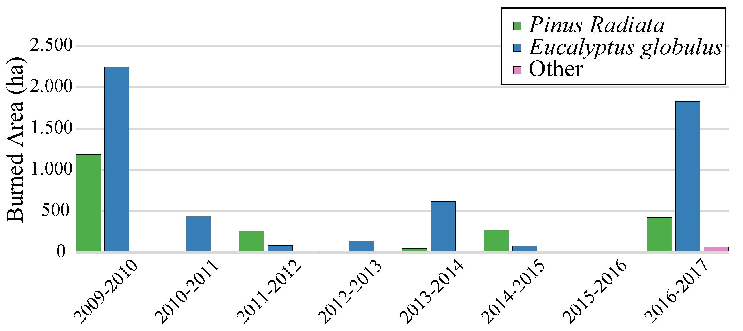
In this work, we analyze the water content of Eucalyptus Globulus and Pinus Radiata using their spectral signature, motivated by the lack of information about these two species in the WUI of Valparaiso. As expected, being dominant species in the forest plantation inventory, the area burned in recent years is more representative in both species, as shown in Figure 2 [34]. For each species, a total of 90 samples were used to measure the spectral reflectance and the mass at different stages of dehydration and senescence. A novel aspect of this work is that we present an evolution of several spectral indexes used in remote sensing for the estimation of biomass moisture content as a function of drying time and residual moisture content. It is expected that the methodologies and the data we present will be a contribution to the wildfire community working on remote sensing tools. Finally, this work is part of the project Understanding Wildfire Hazards Posed by Ignition in Continuous and Discontinuous Configurations, funded by CONICYT (the Chilean National Science Foundation) in an attempt to understand the wildfire risks of Valparaiso region in Chile.

2. Materials and Methods
The field sampling was carried out from August 2018 to March 2019. Leaf samples were collected from Valparaíso WUI, corresponding to Eucalyptus Globulus and Pinus Radiata. The samples were collected on days without precipitation during the previous 24 h. To maintain the freshness of the leaves, branches were cut and stored in plastic bags as recommended in [36]. Then, in less than one hour, the leaves were separated individually from the branches [37,38,39,40]. In the case of eucalyptus, the measurements were made for each leaf, while for pine, approximately 5 grams of pine needles were used, due to the difficulty of registering the spectral signature of a single needle with the sensors used in this study. A total of 90 samples were employed for each species. Once the fresh leaves were cut, the mass was obtained with a 0.1 mg resolution Kern PFB 120-3 precision balance. Leaf spectral reflectance was measured with a high-resolution ASD mineral spectrometer with a spectral range of 350–2500 nm. To record the spectral reflectance, the contact probe of the ASD spectrometer was placed flush against the sample using a white background (white spectralon). The samples were illuminated using the contact probe with a tungsten filament. The spectrometer calibration was performed every 20 readings to ensure the accuracy of the measurements. The reflectance of the white calibration pattern (white spectralon) was used by the spectrometer to set the base line up and calibrate itself [41].
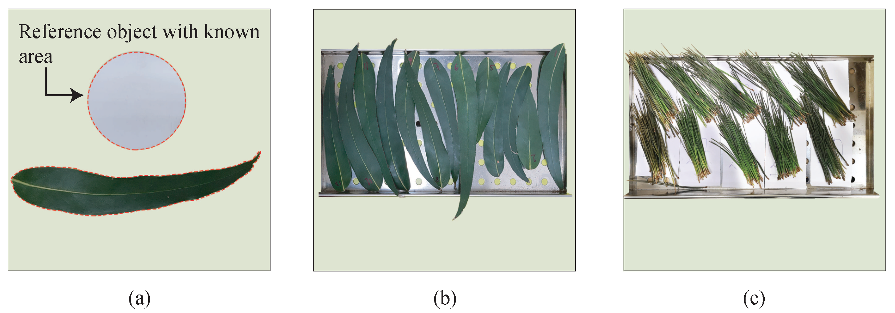
To estimate the area of the eucalyptus leaves, a reference object with a known area was used. A camera (12 MP, f/1.7 aperture with a focal length of 26 mm) was placed twenty centimeters above both samples, to photograph the entire area of the leaf and the reference object. Then, the estimation of the leaf area is calculated as the ratio of the pixels belonging to the leaf and the pixels in the reference object with a known area as shown in Figure 3a.
Next, the fresh leaves were placed in a Memmert UN30 drying oven at 65 C for a fixed time. Figure 3b,c show how the samples were placed in the tray before the dehydration process. Such dehydration temperature was chosen since when assessing the flammability of wildland fuels, it must be ensured that the fuel being analyzed has not lost any flammable content (i.e., that it has not pyrolyzed) so as not to affect the combustion behavior of the samples. The common practice of all combustion scientists working on wildland fuel fire behavior is to dry the samples between 60 and 80 C [42,43,44,45,46,47,48,49]. In the case of eucalyptus, the time was set to 15 min, while for pines the time was 60 min (such time intervals were chosen following the guidelines published in [50,51]). The dehydration process was repeated three times. Then, the leaves were placed in the oven for 24 h at 65 C to obtain constant mass (dry mass) [37,40,52]. Finally, the dry leaves were weighed and the reflectance spectrum was recorded. A detailed description of the instruments used and their specifications are shown in Table 1.
Water Content and Vegetation Indexes
Based on the mass of the leaves at different dehydration stages, the water content is expressed as Fuel Moisture Content (FMC) with fresh——or dry basis——[39,52,53,54] and Equivalent Water Thickness (EWT) [52,53,55,56,57,58]. The former depends only on the leaf mass (Equations (1) and (2)), while the latter also requires its area (Equation (3)):
where (g) is the leaf fresh weight, t is the time in the oven, (g) is the leaf dry weight (after 24 h at 65 C) and A (cm) is the leaf area. To avoid misinterpretations, we refer to FMC just as FMC. As just presented, the water content is obtained during an invasive and time-consuming process of dehydration.
The water content estimation from the spectral signature has been widely studied for a broad variety of vegetation species. Based on the review of the literature, we selected eighteen vegetation indexes that appear frequently in studies related to the use of VIs for the water content estimation (see Table 2 for VIs nomenclatures, references, and a brief description [59,60,61,62,63,64,65,66,67,68,69,70]). For example, in [59] the MSI, NDWI, TM5/TM7, and WI were used to estimate the leaf FMC, and EWT from remotely sensed reflectance. On the other hand, the leaf water status was estimated using the NDWI and the leaf water content index (LWCI) to monitor the forest fire risk [60]. In [61] it is presented the estimation of EWT in eucalyptus leaves using MSI, TM5/TM7, WI, NDWI, and Normalized Difference Vegetation Index (NDVI). However, such eucalyptus species was not Eucalyptus Globulus, and the leaves were not dehydrated. Based on field spectroscopy data, the EWT was estimated using the following indexes WI, SRWI, NDWI, fWBI, SIWSI, and NDII [62]. Also, the same indexes were compared against the use of full-spectrum and continuum removal for leaf-level EWT retrieval in commercial vineyards [63]. In cotton leaves, the EWT and FMC were estimated employing NDII, NDWI1, NDWI2, WI, WBI, fWBI, SRWI, SRWI1, SRWI2, MSI1, MSI2, and SIWSI [64].
3. Results
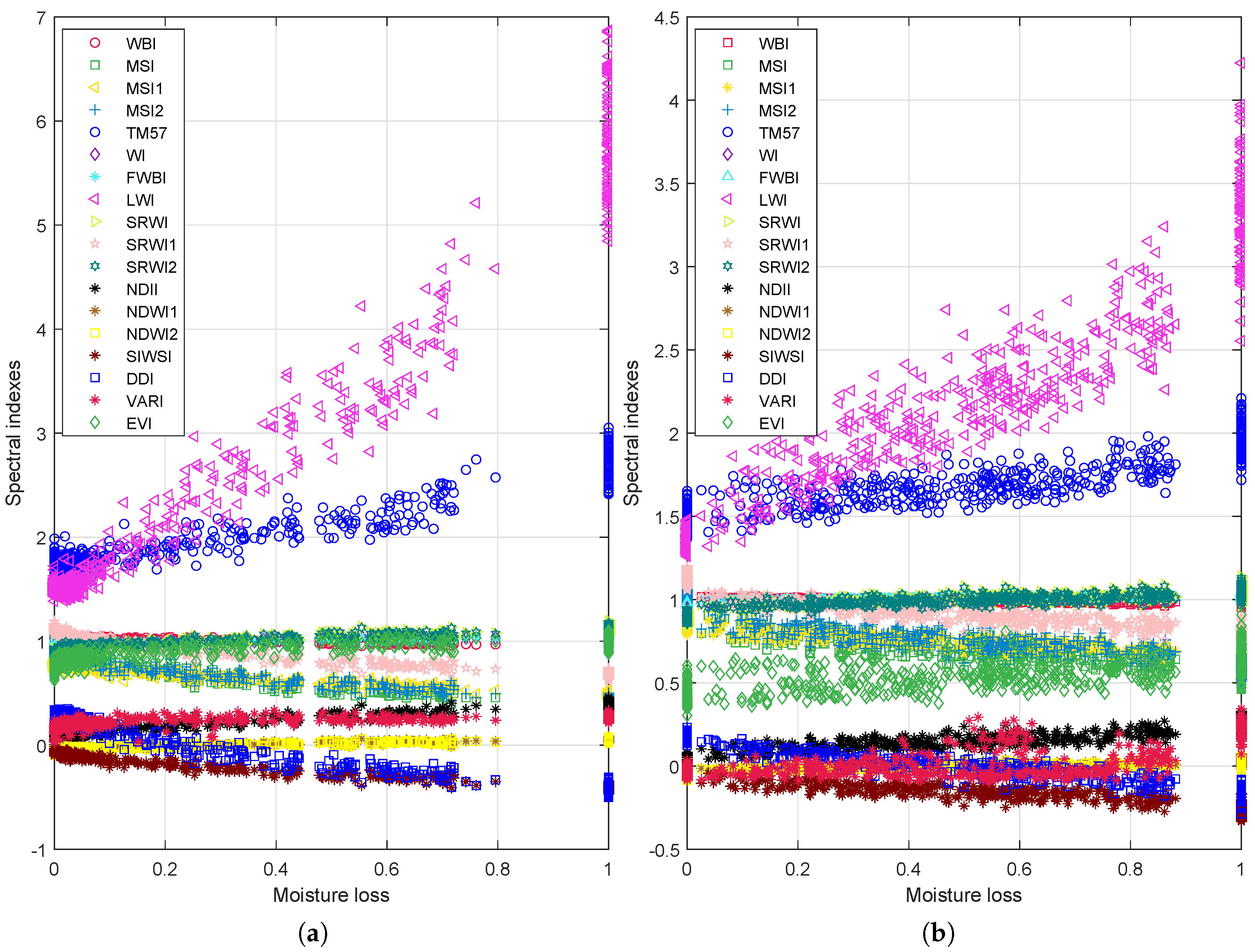
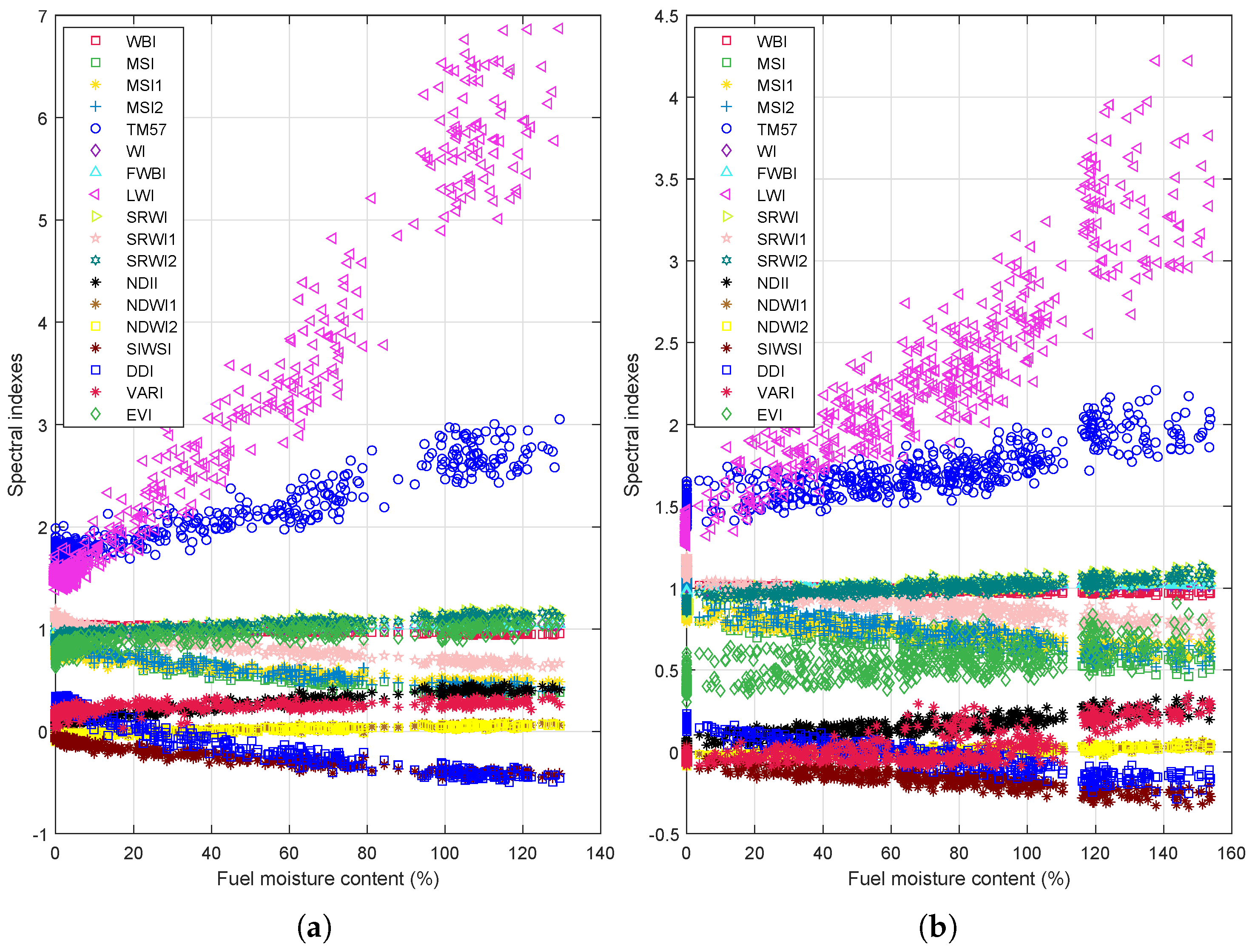
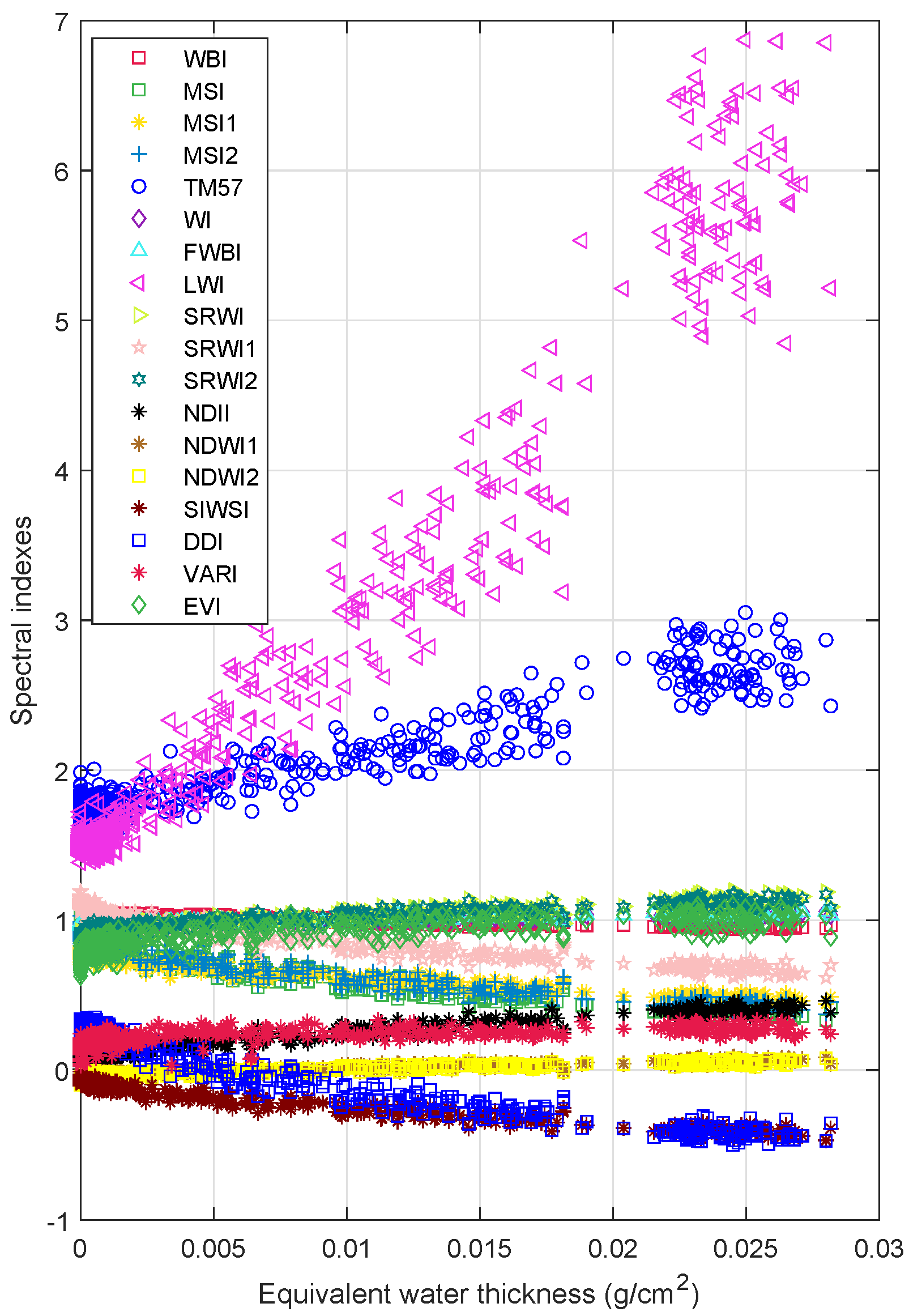
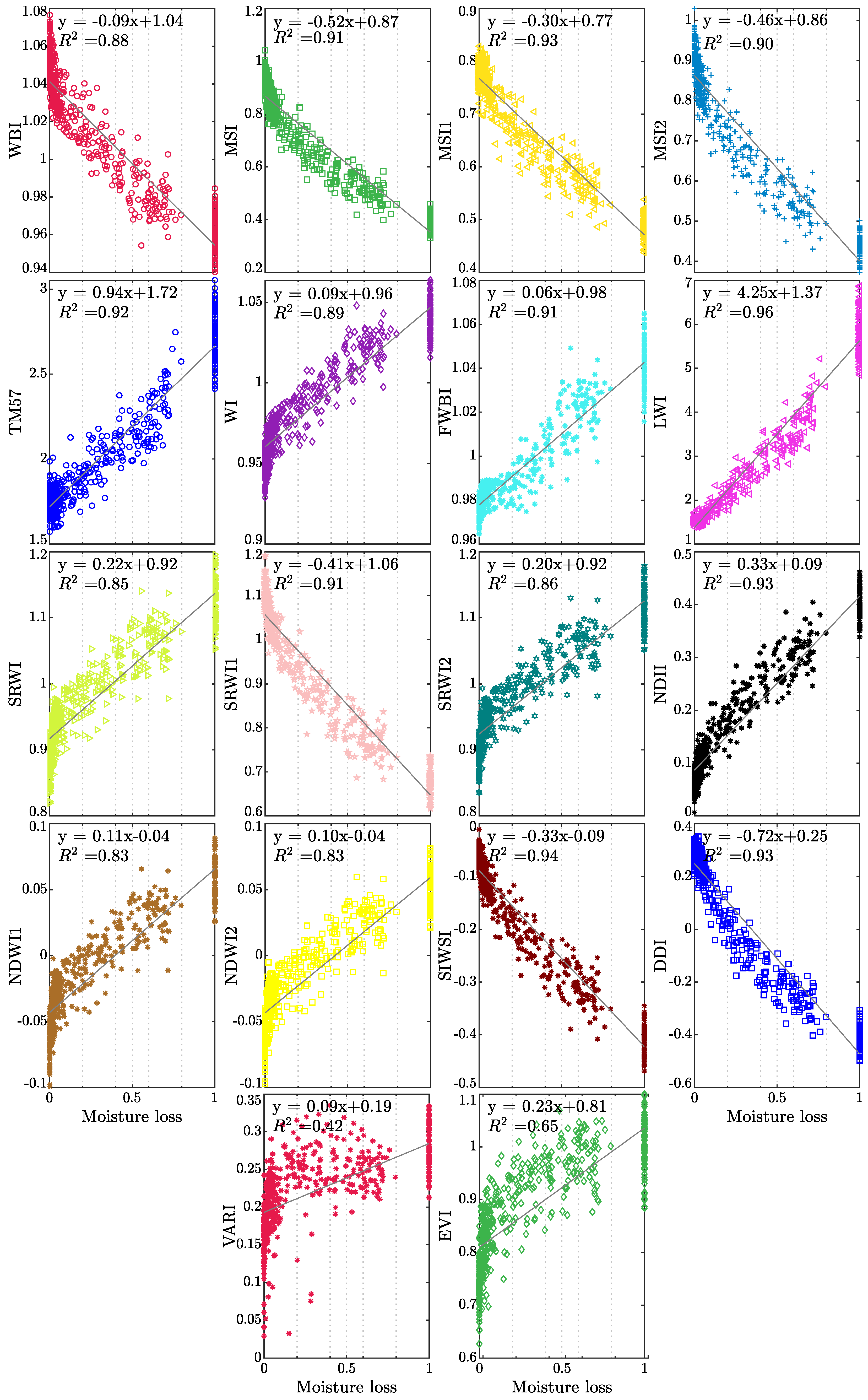
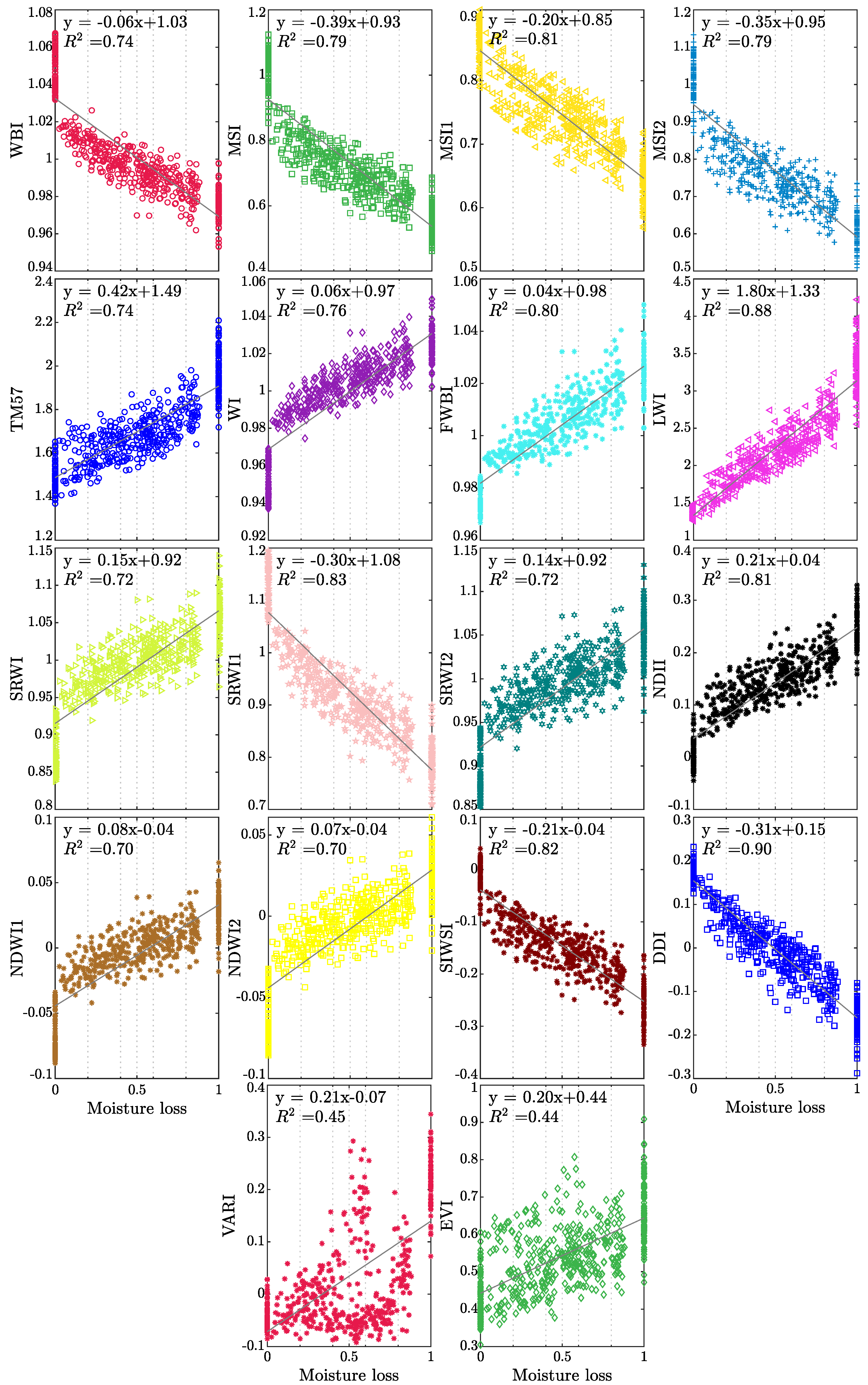
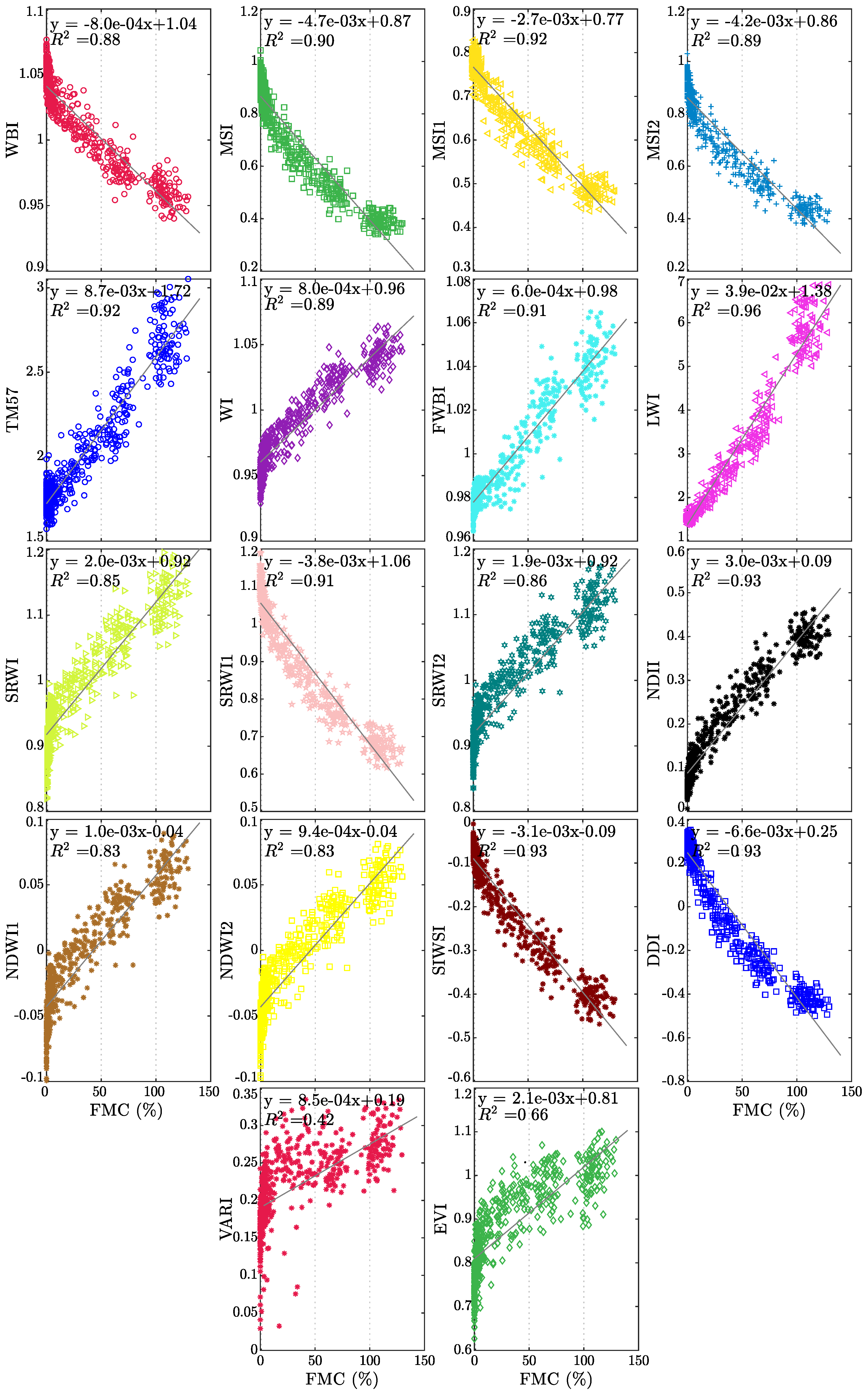
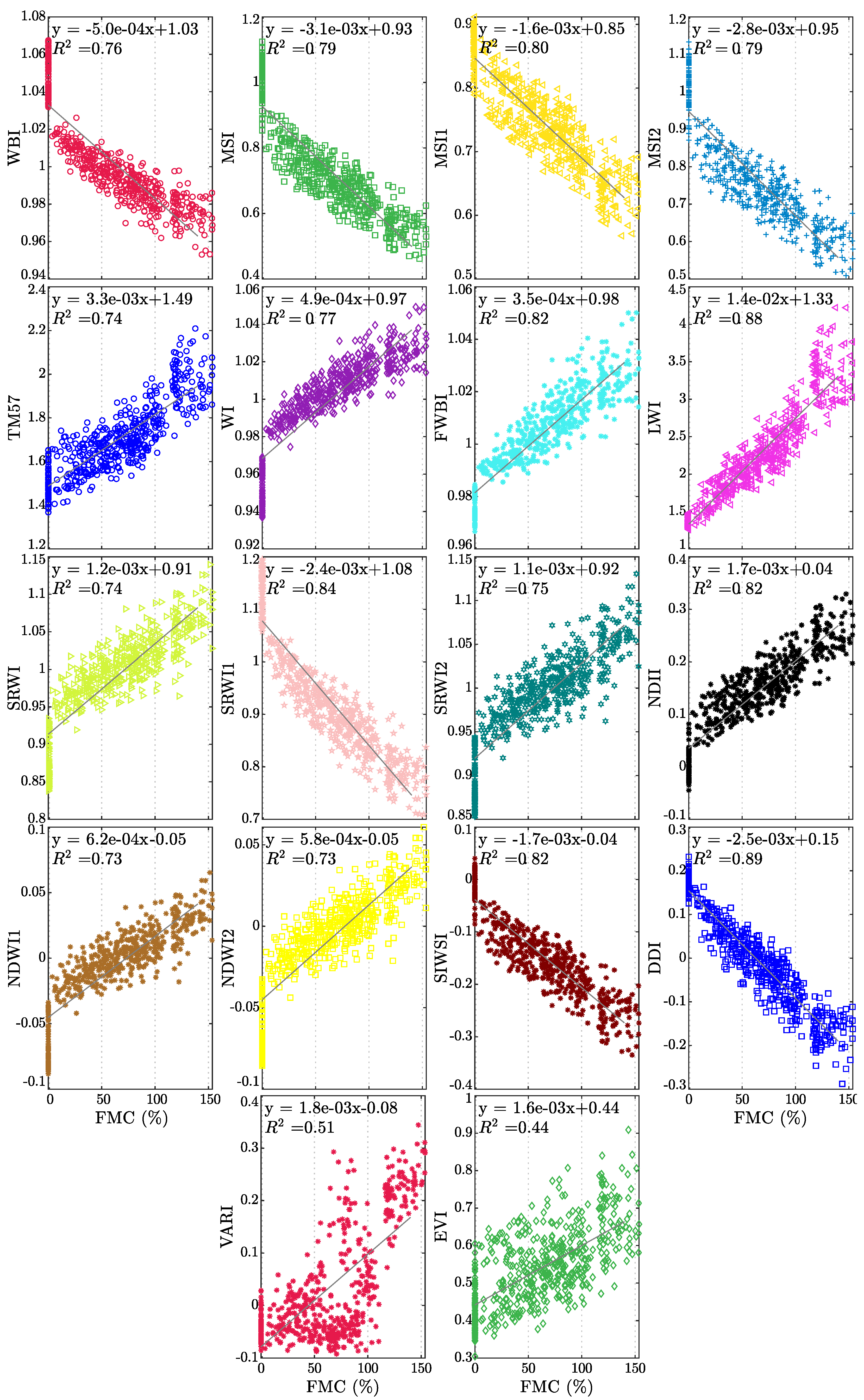
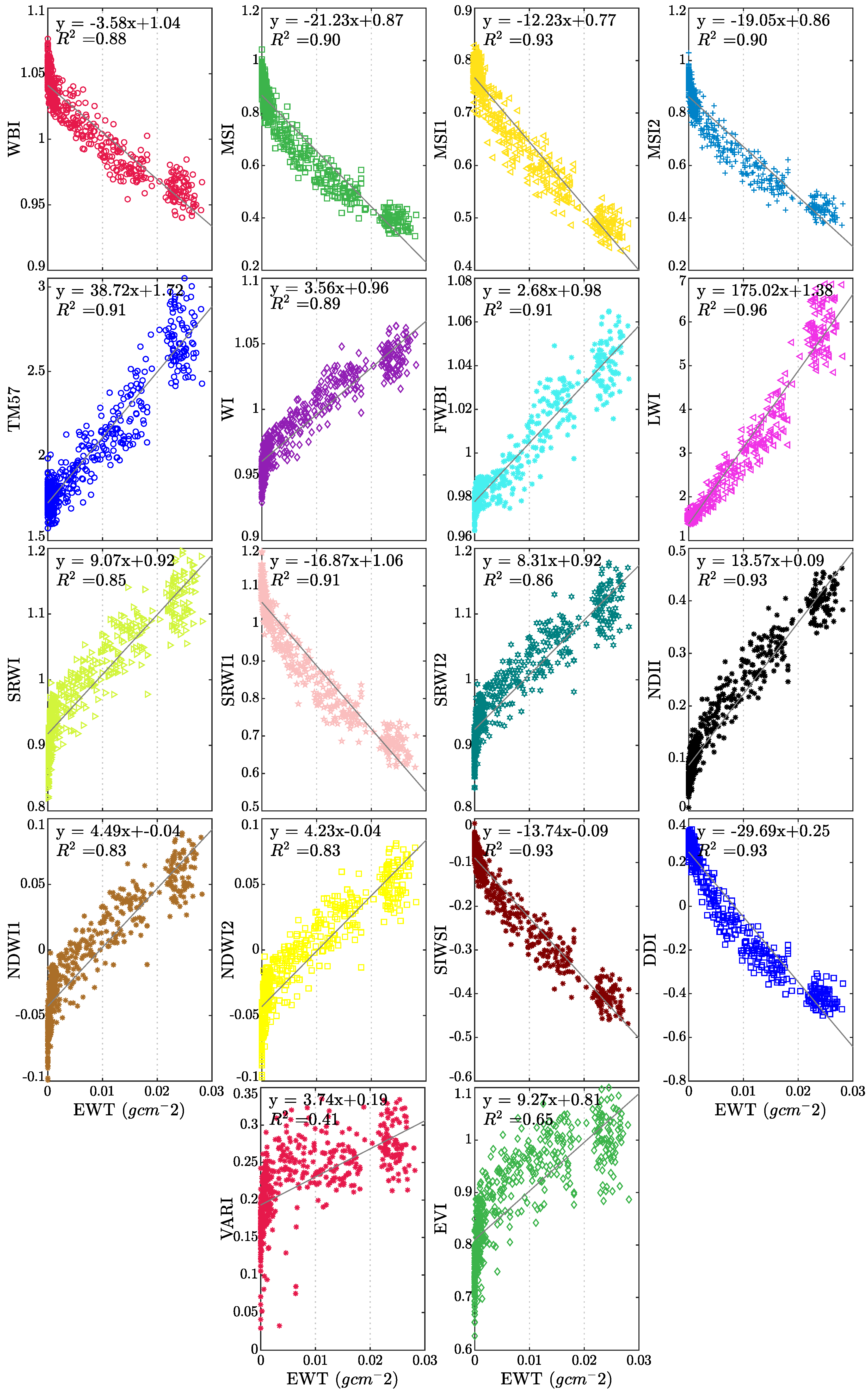
The evolution of the eighteen spectral indexes corresponding to moisture loss for Eucalyptus Globulus and Pinus Radiata is shown in Figure 4. The moisture loss is normalized as the ratio of water contained in each stage of dehydration over the total amount of water. That is, the 0 value means that the leaves do not contain water (after 24 h of drying), meanwhile, the moisture loss 1 represents that the leaves are fresh (recently collected). Figure 5 shows the evolution of the selected vegetation indexes as a function of fuel moisture content (Equation (2)) for eucalyptus and pines. Values of FMC bigger than 100% implies that more than 50% of the leaves’ mass is water. Specifically, the maximum FMC contained in eucalyptus leaves is 129%, whereas the maximum FMC in pine needles is 153%. Finally, the variation of the spectral indexes when the equivalent water thickness of eucalyptus changes is presented in Figure 6. As can be seen in Figure 4, Figure 5 and Figure 6, the dehydration process allows us to have a wide range of values of moisture loss, FMC, and EWT. In addition, the behavior of the eighteen vegetation indexes is proportional to the water indicators. The aforementioned behavior is modeled as a linear regression in Appendix A (Figure A1, Figure A2, Figure A3, Figure A4, Figure A5), where a individual linear model is presented with its corresponding coefficient of determination .
4. Discussion
Figure 4, Figure 5 and Figure 6 suggest that the relationship between the leaf water content (expressed in terms of: moisture loss, , and EWT) and spectral indexes, for both species, is linear. In particular Figure A1 and Figure A2 evidence that all spectral indexes appeared to behave linearly with a of in the worst case—VARI index for EWT estimation in eucalyptus—and of in the best case—LWI index for moisture loss and EWT for eucalyptus—These values are similar to values founded in previous works [22,24,26,27,29,75], yet these works assessed the water content of others species.
The indexes with the lowest values—VARI 0.41 for EWT and EVI 0.44 for FMC and moisture loss—could advise that the index behavior is not linear. Nonetheless, the main reason can be associated with the dispersion of index values; the fitted model does not consider their variance. Specifically, the indexes derived from Pinus Radiata leaves present the biggest variations, as can be appreciated in Figure A2 and Figure A4. The variance of the index values shows that the Pinus Radiata leaves did not dry uniformly because of their initial water content and arrangement in the trail (sets of 5 g). Nevertheless, despite these issues, the robustness of the indexes can be inferred based on the variance and value. In particular, the indexes that showed the greater values are LWI and DDI, DDI achieved the greater value. Therefore, the behavior of spectral indexes and linear regression advise that the most suitable index to assess the water content in acicular leaves (Pinus Radiata leaves) is DDI.
Regarding to Eucalyptus Globulus leaves, the linear relationship between water content (moisture loss, , and EWT)) and spectral indexes is more evident for this specie, reaching an value of , see Figure A1, Figure A3 and Figure A5. Moreover, the distribution of index values is narrower than the values obtained for Pinus Radiata. This suggest that the samples arrangement (see Figure 3) and drying process performed better than for non acicular leaves.
For both species (Eucalyptus Globulus, Pinus Radiata), the initial conditions of leaves can explain the index values dispersion. When the leaves were taken, it was assumed that all leaves samples had the same water status. Nevertheless, this is not always the case since the samples were taken randomly from several branches on different locations and environmental conditions (the only constraint considered was the absence of rain at least 24 h before taking the samples). Thus, the initial water status for the samples was not all the same. Then, at each dehydration stage, the leaves samples did not dry at the same level. On the other side, it is to be noted that we have not performed yet a correlation between the geographical location of the samples, the climate conditions, water status (FMC, EWT) and the eighteen vegetation indexes obtained.
In brief, despite the index values dispersion issue, results showed that water status in leaves can be assessed in different dehydration stages by the reflectance of leaves.
5. Conclusions
This work has shown the results of analyzing the spectral signature (at different dehydration levels) of the two most prevalent species in Valparaíso region, Chile, within the research project Understanding Wildfire Hazards Posed by Ignition in Continuous and Discontinuous Configurations, funded by CONICYT (the Chilean National Science Foundation), as an attempt to understand wildfire risks. The two species studied were Eucalyptus Globulus and Pinus Radiata, which represent the 97.5% of the vegetation. The samples were randomly collected from different locations and eighteen vegetation indexes—namely: WBI, MSI, MSI1, MSI2, TM5/TM7, WI, fWBI, LWI, SRWI, SRWI1, SRWI2, NDII, NDWI1, NDWI2, SIWSI, DDI, VARI, and EVI—were determined. We found that such indexes behave linearly under moisture loss and fuel moisture content estimation. In particular, LWI and DDI index have performed the best linear behavior for each species (Eucalyptus Globulus, Pinus Radiata), respectively. LWI reach an in all water status characterizations (moisture, , and EWT), and DDI achieved a for moisture loss and for . Moreover, these indexes showed the lowest dispersion. Therefore, the assessment of wildfire risk behavior can be further enhanced by the behavior of each spectral index showed in the present work and can be extended to other research fields, such as agriculture.
Author Contributions
Conceptualization, F.A.C., A.F. and P.R.; methodology, J.V. and T.A.-R.; software, J.V. and T.A.-R.; validation, J.V. and T.A.-R.; formal analysis, F.A.C., J.V. and T.A.-R.; investigation, J.V. and T.A.-R.; resources, F.A.C. and A.F.; data curation, A.F. and P.R.; writing—original draft preparation, J.V., T.A.-R., F.A.C., A.F. and P.R.; writing—review and editing, F.A.C. and A.F.; visualization, J.V. and T.A.-R.; supervision, F.A.C.; project administration, A.F.
Funding
The authors would like to thank to CONICYT PIA/ANILLO ACT172095, CONICYT FB0008 and CONICYT FONDECYT 1171431. Authors would also like to thank to Universidad Técnica Federico Santa María, DGIIP, PIIC 29/2019, Universidad Adolfo Ibáñez, and CONICYT PFCHA/DoctoradoNacional/2019-21190471.
Acknowledgments
The authors would like to thank to Gonzalo Olivares for his assistance during the research.
Conflicts of Interest
The authors declare no conflict of interest.
Appendix A. Linear Regression Fitting of Indexes
Figure A1.
Linear regression of the moisture loss and the vegetation indexes for the Eucalyptus Globulus.
Figure A1.
Linear regression of the moisture loss and the vegetation indexes for the Eucalyptus Globulus.

Figure A2.
Linear regression of the moisture loss and the vegetation indexes for the Pinus Radiata.

Figure A3.
Linear regression of the fuel moisture content and the vegetation indexes for the Eucalyptus Globulus.
Figure A3.
Linear regression of the fuel moisture content and the vegetation indexes for the Eucalyptus Globulus.

Figure A4.
Linear regression of the fuel moisture content and the vegetation indexes for the Pinus Radiata.
Figure A4.
Linear regression of the fuel moisture content and the vegetation indexes for the Pinus Radiata.

Figure A5.
Linear regression of the equivalent water thickness for the Eucalyptus Globulus case.

References
- Reszka, P.; Fuentes, A. The Great Valparaiso Fire and Fire Safety Management in Chile. Fire Technol. 2015, 51, 753–758. [Google Scholar] [CrossRef] [Green Version]
- Soto, M.C.; Julio-Alvear, G.; Salinas, R.G. Chapter 4—Current Wildfire Risk Status and Forecast in Chile: Progress and Future Challenges. In Wildfire Hazards, Risks and Disasters; Shroder, J.F., Paton, D., Eds.; Elsevier: Oxford, UK, 2015; pp. 59–75. [Google Scholar] [CrossRef]
- Conaf, C.N.F. Estadísticas-Resumen Regional Ocurrencia (Número) y Daño (Superficie Afectada) por Incendios Forestales 1977–2018; Programa de Manejo del Fuego; Corporación Nacionial Forestal: Santiago, Chile, 2018. [Google Scholar]
- Heilmayr, R.; Echeverria, C.; Fuentes, R.; Lambin, E.F. A plantation-dominated forest transition in Chile. Appl. Geogr. 2016, 75, 71–82. [Google Scholar] [CrossRef] [Green Version]
- Gysling Caselli, A.J.; Alvarez González, V.; Soto Aguirre, D.A.; Pardo, V.; Poblete, P. Anuario Forestal 2018. In Chilean Statistical Yearbook of Forestry; INFOR: Santiago, Chile, 2018; Volume 163. [Google Scholar]
- Conaf, C.N.F. Estadísticas-Causas según Ocurrencia de Incendios Forestales 1987–2018; Programa de Manejo del Fuego; Corporación Nacionial Forestal: Santiago, Chile, 2018. [Google Scholar]
- Sección de Análisis y Predicción de Incendios Forestales CONAF—Frecuencia Incendios Forestales (2002–2019). Available online: https://conaf.carto.com/u/geprif (accessed on 24 May 2019).
- Rougier, J.; Sparks, S.; Hill, L. Risk and Uncertainty Assessment for Natural Hazards; Cambridge University Press: Cambridge, UK, 2013. [Google Scholar] [CrossRef]
- Vitolo, C.; Di Giuseppe, F.; Krzeminski, B.; San-Miguel-ayanz, J. Data descriptor: A 1980–2018 global fire danger re-analysis dataset for the Canadian fire weather indices. Sci. Data 2019, 6. [Google Scholar] [CrossRef] [PubMed]
- Mahmoud, H.; Chulahwat, A. Unraveling the Complexity of Wildland Urban Interface Fires. Sci. Rep. 2018, 8, 9315. [Google Scholar] [CrossRef] [PubMed] [Green Version]
- Fernandez-Pello, A.C. Wildland fire spot ignition by sparks and firebrands. Fire Saf. J. 2017, 91, 2–10. [Google Scholar] [CrossRef]
- Baines, P.G. Physical mechanisms for the propagation of surface fires. Math. Comput. Model. 1990, 13, 83–94. [Google Scholar] [CrossRef]
- Rossa, C.G.; Fernandes, P.M. Live Fuel Moisture Content: The ‘Pea Under the Mattress’ of Fire Spread Rate Modeling? Fire 2018, 1, 43. [Google Scholar] [CrossRef] [Green Version]
- Lawson, B.; Hawkes, B. Field evaluation of a moisture content model for medium-sized logging slash. In Proceedings of the 10th Conference on Fire and Forest Meteorology, Ottawa, ON, Canada, 17–21 April 1989; pp. 247–257. [Google Scholar]
- Yebra, M.; Dennison, P.; Chuvieco, E.; Riaño, D.; Zylstra, P.; Hunt, E.; Danson, F.; Qi, Y.; Jurdao, S. A global review of remote sensing of live fuel moisture content for fire danger assessment: Moving towards operational products. Remote Sens. Environ. 2013, 136, 455–468. [Google Scholar] [CrossRef]
- Yebra, M.; Quan, X.; Riaño, D.; Rozas Larraondo, P.; van Dijk, A.; Cary, G. A fuel moisture content and flammability monitoring methodology for continental Australia based on optical remote sensing. Remote Sens. Environ. 2018, 212, 260–272. [Google Scholar] [CrossRef]
- Quan, X.; He, B.; Yebra, M.; Yin, C.; Liao, Z.; Li, X. Retrieval of forest fuel moisture content using a coupled radiative transfer model. Environ. Model. Softw. 2017, 95, 290–302. [Google Scholar] [CrossRef]
- Peñuelas, J.; Filella, I.; Biel, C.; Serrano, L.; Save, R. The reflectance at the 950–970 nm region as an indicator of plant water status. Int. J. Remote Sens. 1993, 14, 1887–1905. [Google Scholar] [CrossRef]
- Hunt, E.R., Jr.; Rock, B.N. Detection of changes in leaf water content using near-and middle-infrared reflectances. Remote Sens. Environ. 1989, 30, 43–54. [Google Scholar] [CrossRef]
- Rock, B.N.; Vogelmann, J.E.; Williams, D. Field and airborne spectral characterization of suspected damage in red spruce (Picea rubens) from vermont. Remote Sens. Environ. 1985, 30, 71–81. [Google Scholar]
- Rock, B.; Vogelmann, J.; Williams, D.; Vogelmann, A.; Hoshizaki, T. Remote Detection of Forest Damage: Plant responses to stress may have spectral “signatures” that could be used to map, monitor, and measure forest damage. Bioscience 1986, 36, 439–445. [Google Scholar] [CrossRef]
- Elvidge, C.D.; Lyon, R.J. Estimation of the vegetation contribution to the 1· 65/2· 22 μm ratio in airborne thematic-mapper imagery of the Virginia Range, Nevada. Int. J. Remote Sens. 1985, 6, 75–88. [Google Scholar] [CrossRef]
- Peñuelas, J.; Pinol, J.; Ogaya, R.; Filella, I. Estimation of plant water concentration by the reflectance water index WI (R900/R970). Int. J. Remote Sens. 1997, 18, 2869–2875. [Google Scholar] [CrossRef]
- Zarco-Tejada, P.J.; Ustin, S. Modeling canopy water content for carbon estimates from MODIS data at land EOS validation sites. In Proceedings of the IGARSS 2001 Scanning the Present and Resolving the Future. IEEE 2001 International Geoscience and Remote Sensing Symposium (Cat. No. 01CH37217), Sydney, NSW, Australia, 9–13 July 2001; Volume 1, pp. 342–344. [Google Scholar]
- Gao, B.C. NDWI—A normalized difference water index for remote sensing of vegetation liquid water from space. Remote Sens. Environ. 1996, 58, 257–266. [Google Scholar] [CrossRef]
- Seelig, H.D.; Hoehn, A.; Stodieck, L.; Klaus, D.; Adams Iii, W.; Emery, W. The assessment of leaf water content using leaf reflectance ratios in the visible, near-, and short-wave-infrared. Int. J. Remote Sens. 2008, 29, 3701–3713. [Google Scholar] [CrossRef]
- Rodríguez-Pérez, J.R.; Riaño, D.; Carlisle, E.; Ustin, S.; Smart, D.R. Evaluation of hyperspectral reflectance indexes to detect grapevine water status in vineyards. Am. J. Enol. Vitic. 2007, 58, 302–317. [Google Scholar]
- Wang, Q.; Li, P. Hyperspectral indices for estimating leaf biochemical properties in temperate deciduous forests: Comparison of simulated and measured reflectance data sets. Ecol. Indic. 2012, 14, 56–65. [Google Scholar] [CrossRef]
- Hardisky, M.; Klemas, V.; Smart, M. The influence of soil salinity, growth form, and leaf moisture on the spectral radiance of. Spartina Alterniflora 1983, 49, 77–83. [Google Scholar]
- Fensholt, R.; Sandholt, I. Derivation of a shortwave infrared water stress index from MODIS near-and shortwave infrared data in a semiarid environment. Remote Sens. Environ. 2003, 87, 111–121. [Google Scholar] [CrossRef]
- Gitelson, A.; Kaufman, Y.; Stark, R.; Rundquist, D. Novel algorithms for remote estimation of vegetation fraction. Remote Sens. Environ. 2002, 80, 76–87. [Google Scholar] [CrossRef] [Green Version]
- Clevers, J.; Kooistra, L.; Schaepman, M. Estimating canopy water content using hyperspectral remote sensing data. Int. J. Appl. Earth Obs. Geoinf. 2010, 12, 119–125. [Google Scholar] [CrossRef]
- Jurdao, S.; Yebra, M.; Guerschman, J.; Chuvieco, E. Regional estimation of woodland moisture content by inverting Radiative Transfer Models. Remote Sens. Environ. 2013, 132, 59–70. [Google Scholar] [CrossRef]
- Conaf, C.N.F. Estadísticas-Ocurrencia y Daño por Incendios Forestales según Incendios de Magnitud 1985–2018; Programa de Manejo del Fuego; Corporación Nacionial Forestal: Santiago, Chile, 2018. [Google Scholar]
- Conaf, C.N.F.; Conama, C.N.d.M.A. Plantación Forestal; Chilean Forest Service: Santiago, Chile, 1997. [Google Scholar]
- Kumar, L. High-spectral resolution data for determining leaf water content in Eucalyptus species: Leaf level experiments. Geocarto Int. 2007, 22, 3–16. [Google Scholar] [CrossRef]
- Zarco-Tejada, P.J.; Rueda, C.; Ustin, S.L. Water content estimation in vegetation with MODIS reflectance data and model inversion methods. Remote Sens. Environ. 2003, 85, 109–124. [Google Scholar] [CrossRef]
- Madrigal, J.; Hernando, C.; Guijarro, M. A new bench-scale methodology for evaluating the flammability of live forest fuels. J. Fire Sci. 2013, 31, 131–142. [Google Scholar] [CrossRef]
- Qi, Y.; Dennison, P.E.; Jolly, W.M.; Kropp, R.C.; Brewer, S.C. Spectroscopic analysis of seasonal changes in live fuel moisture content and leaf dry mass. Remote Sens. Environ. 2014, 150, 198–206. [Google Scholar] [CrossRef] [Green Version]
- Chelli, S.; Maponi, P.; Campetella, G.; Monteverde, P.; Foglia, M.; Paris, E.; Lolis, A.; Panagopoulos, T. Adaptation of the Canadian fire weather index to Mediterranean forests. Nat. Hazards 2015, 75, 1795–1810. [Google Scholar] [CrossRef]
- TerraSpec User Manual. Available online: https://www.mapping-solutions.co.uk/downloads/data/pdf/A1044.pdf (accessed on 7 October 2019).
- Trabaud, L. Inflammabilité et combustibilité des principales espèces des garrigues de la région méditerranéenne. Oecologia Plant 1976, 11, 117–136. [Google Scholar]
- Caramelle, P.; Clément, A. Inflammabilité et Combustibilité de la Végétation Méditerrannéene; Institut National de la Recherche Agronomique (I.N.R.A.): Avignon, France, 1978. [Google Scholar]
- Valette, J. Inflammabilité, teneur en eau et turgescence relative de quatre espèces forestières méditerranéennes. In Documentos del Seminario sobre Métodos y Equipos para la Prevención de Incendios Forestales; Instituto Nacional para la Conservación de la Naturaleza, MAPA: Madrid, Spain, 1988; pp. 98–107. [Google Scholar]
- Elvira Martín, L.M.; Hernando Lara, C. Inflamabilidad y Energía de las Especies de Sotobosque; Instituto Nacional de Investigaciones Agrarias (INIA), Ministerio de Agricultura, Pesca y Alimentación: Madrid, Spain, 1989. [Google Scholar]
- Desbois, N.; Pereira, J.; Beaudoin, A.; Chuvieco, E.; Vidal, A. Short term fire risk mapping using remote sensing. In A Review of Remote Sensing Methods for the Study of Large Wildland Fires; Chuvieco, E., Ed.; Megafires Project ENV-CT96-0256: Alcalá de Henares, Spain, 1997; pp. 29–60. [Google Scholar]
- Asner, G.P.; Martin, R.E.; Tupayachi, R.; Emerson, R.; Martinez, P.; Sinca, F.; Powell, G.V.; Wright, S.J.; Lugo, A.E. Taxonomy and remote sensing of leaf mass per area (LMA) in humid tropical forests. Ecol. Appl. 2011, 21, 85–98. [Google Scholar] [CrossRef] [PubMed]
- Simeoni, A.; Thomas, J.; Bartoli, P.; Borowieck, P.; Reszka, P.; Colella, F.; Santoni, P.A.; Torero, J.L. Flammability studies for wildland and wildland–urban interface fires applied to pine needles and solid polymers. Fire Saf. J. 2012, 54, 203–217. [Google Scholar] [CrossRef] [Green Version]
- Jervis, F.X.; Rein, G. Experimental study on the burning behaviour of Pinus halepensis needles using small-scale fire calorimetry of live, aged and dead samples. Fire Mater. 2016, 40, 385–395. [Google Scholar] [CrossRef] [Green Version]
- Liu, N.; Wu, L.; Chen, L.; Sun, H.; Dong, Q.; Wu, J. Spectral Characteristics Analysis and Water Content Detection of Potato Plants Leaves. IFAC-PapersOnLine 2018, 51, 541–546. [Google Scholar] [CrossRef]
- Gameiro, C.; Utkin, A.; Cartaxana, P.; da Silva, J.M.; Matos, A. The use of laser induced chlorophyll fluorescence (LIF) as a fast and non-destructive method to investigate water deficit in Arabidopsis. Agric. Water Manag. 2016, 164, 127–136. [Google Scholar] [CrossRef]
- Ceccato, P.; Flasse, S.; Tarantola, S.; Jacquemoud, S.; Grégoire, J.M. Detecting vegetation leaf water content using reflectance in the optical domain. Remote Sens. Environ. 2001, 77, 22–33. [Google Scholar] [CrossRef]
- Cao, Z.; Wang, Q. Retrieval of leaf fuel moisture contents from hyperspectral indices developed from dehydration experiments. Eur. J. Remote Sens. 2017, 50, 18–28. [Google Scholar] [CrossRef] [Green Version]
- Wei, Y.; Wu, F.; Xu, J.; Sha, J.; Zhao, Z.; He, Y.; Li, X. Visual detection of the moisture content of tea leaves with hyperspectral imaging technology. J. Food Eng. 2019, 248, 89–96. [Google Scholar] [CrossRef]
- De Jong, S.M.; Addink, E.A.; Doelman, J.C. Detecting leaf-water content in Mediterranean trees using high-resolution spectrometry. Int. J. Appl. Earth Obs. Geoinf. 2014, 27, 128–136. [Google Scholar] [CrossRef]
- González-Fernández, A.B.; Rodríguez-Pérez, J.R.; Marcelo, V.; Valenciano, J.B. Using field spectrometry and a plant probe accessory to determine leaf water content in commercial vineyards. Agric. Water Manag. 2015, 156, 43–50. [Google Scholar] [CrossRef]
- El-Hendawy, S.E.; Al-Suhaibani, N.A.; Elsayed, S.; Hassan, W.M.; Dewir, Y.H.; Refay, Y.; Abdella, K.A. Potential of the existing and novel spectral reflectance indices for estimating the leaf water status and grain yield of spring wheat exposed to different irrigation rates. Agric. Water Manag. 2019, 217, 356–373. [Google Scholar] [CrossRef]
- Cao, Z.; Wang, Q.; Zheng, C. Best hyperspectral indices for tracing leaf water status as determined from leaf dehydration experiments. Ecol. Indic. 2015, 54, 96–107. [Google Scholar] [CrossRef]
- Danson, F.; Bowyer, P. Estimating live fuel moisture content from remotely sensed reflectance. Remote Sens. Environ. 2004, 92, 309–321. [Google Scholar] [CrossRef]
- Maki, M.; Ishiahra, M.; Tamura, M. Estimation of leaf water status to monitor the risk of forest fires by using remotely sensed data. Remote Sens. Environ. 2004, 90, 441–450. [Google Scholar] [CrossRef]
- Datt, B. Remote sensing of water content in Eucalyptus leaves. Aust. J. Bot. 1999, 47, 909–923. [Google Scholar] [CrossRef]
- Rodríguez-Pérez, J.; Ordóñez, C.; González-Fernández, A.; Sanz-Ablanedo, E.; Valenciano, J.; Marcelo, V. Leaf water content estimation by functional linear regression of field spectroscopy data. Biosyst. Eng. 2018, 165, 36–46. [Google Scholar] [CrossRef]
- Fang, M.; Ju, W.; Zhan, W.; Cheng, T.; Qiu, F.; Wang, J. A new spectral similarity water index for the estimation of leaf water content from hyperspectral data of leaves. Remote Sens. Environ. 2017, 196, 13–27. [Google Scholar] [CrossRef]
- Yi, Q.X.; Bao, A.M.; Wang, Q.; Zhao, J. Estimation of leaf water content in cotton by means of hyperspectral indices. Comput. Electron. Agric. 2013, 90, 144–151. [Google Scholar] [CrossRef]
- González-Fernández, A.; Rodríguez-Pérez, J.; Marabel, M.; Álvarez Taboada, F. Spectroscopic estimation of leaf water content in commercial vineyards using continuum removal and partial least squares regression. Sci. Hortic. 2015, 188, 15–22. [Google Scholar] [CrossRef]
- Kovar, M.; Brestic, M.; Sytar, O.; Barek, V.; Hauptvogel, P.; Zivcak, M. Evaluation of hyperspectral reflectance parameters to assess the leafwater content in soybean. Water 2019, 11, 443. [Google Scholar] [CrossRef] [Green Version]
- Chen, D.; Huang, J.; Jackson, T. Vegetation water content estimation for corn and soybeans using spectral indices derived from MODIS near- and short-wave infrared bands. Remote Sens. Environ. 2005, 98, 225–236. [Google Scholar] [CrossRef]
- Davidson, A.; Wang, S.; Wilmshurst, J. Remote sensing of grassland-shrubland vegetation water content in the shortwave domain. Int. J. Appl. Earth Obs. Geoinf. 2006, 8, 225–236. [Google Scholar] [CrossRef]
- Lei, J.; Yang, W.; Li, H.; Wu, M.; She, J.; Zhou, X.; Huang, B.; Zhang, Y.; Liu, L.; Luo, X. Leaf equivalent water thickness assessment by means of spectral analysis and a new vegetation index. J. Appl. Remote Sens. 2019, 13. [Google Scholar] [CrossRef]
- Han, D.; Liu, S.; Du, Y.; Xie, X.; Fan, L.; Lei, L.; Li, Z.; Yang, H.; Yang, G. Crop Water Content of Winter Wheat Revealed with Sentinel-1 and Sentinel-2 Imagery. Sensors 2019, 19, 4013. [Google Scholar] [CrossRef] [Green Version]
- Strachan, I.B.; Pattey, E.; Boisvert, J.B. Impact of nitrogen and environmental conditions on corn as detected by hyperspectral reflectance. Remote Sens. Environ. 2002, 80, 213–224. [Google Scholar] [CrossRef]
- Le Maire, G.; Francois, C.; Dufrene, E. Towards universal broad leaf chlorophyll indices using PROSPECT simulated database and hyperspectral reflectance measurements. Remote Sens. Environ. 2004, 89, 1–28. [Google Scholar] [CrossRef]
- Caccamo, G.; Chisholm, L.; Bradstock, R.; Puotinen, M.; Pippen, B. Monitoring live fuel moisture content of heathland, shrubland and sclerophyll forest in south-eastern Australia using MODIS data. Int. J. Wildl. Fire 2012, 21, 257–269. [Google Scholar] [CrossRef]
- Stow, D.; Niphadkar, M.; Kaiser, J. MODIS-derived visible atmospherically resistant index for monitoring chaparral moisture content. Int. J. Remote Sens. 2005, 26, 3867–3873. [Google Scholar] [CrossRef]
- Roberts, D.; Dennison, P.; Peterson, S.; Sweeney, S.; Rechel, J. Evaluation of Airborne Visible/Infrared Imaging Spectrometer (AVIRIS) and Moderate Resolution Imaging Spectrometer (MODIS) measures of live fuel moisture and fuel condition in a shrubland ecosystem in southern California. J. Geophys. Res. Biogeosci. 2006, 111. [Google Scholar] [CrossRef] [Green Version]
- Gao, X.; Huete, A.R.; Ni, W.; Miura, T. Optical–biophysical relationships of vegetation spectra without background contamination. Remote Sens. Environ. 2000, 74, 609–620. [Google Scholar] [CrossRef]
Figure 2.
Hectares burned of Valparaiso’s forest plantation during 2009–2017 [34].
Figure 2.
Hectares burned of Valparaiso’s forest plantation during 2009–2017 [34].

Figure 3.
Leaves disposition before dehydration process. (a) shows the reference object used to estimate leaves’ area; (b,c) show the leaves on the tray as captured by the camera.
Figure 3.
Leaves disposition before dehydration process. (a) shows the reference object used to estimate leaves’ area; (b,c) show the leaves on the tray as captured by the camera.

Figure 4.
Relationship between moisture loss and the vegetation indexes. (a) shows the results for the Eucalyptus Globulus case, and (b) for the Pinus Radiata case.
Figure 4.
Relationship between moisture loss and the vegetation indexes. (a) shows the results for the Eucalyptus Globulus case, and (b) for the Pinus Radiata case.

Figure 5.
Relationship between fuel moisture content (FMC) and the vegetation indexes. The FMC with dry basis is calculated according to Equation (1). (a) shows the results for the Eucalyptus Globulus case, whereas (b) shows the results for the Pinus Radiata case.
Figure 5.
Relationship between fuel moisture content (FMC) and the vegetation indexes. The FMC with dry basis is calculated according to Equation (1). (a) shows the results for the Eucalyptus Globulus case, whereas (b) shows the results for the Pinus Radiata case.

Figure 6.
Relationship between equivalent water thickness (EWT) and Eucalyptus Globulus vegetation indexes. The EWT is calculated according to Equation (3).
Figure 6.
Relationship between equivalent water thickness (EWT) and Eucalyptus Globulus vegetation indexes. The EWT is calculated according to Equation (3).


Table 1.
Technical Specifications of the instruments used in the procedure.
| Instrument | Technical Specifications |
|---|---|
| TerraSpec 4 Hi-Res Mineral spectrometer | Wavelength range: 350–2500 nm |
| Resolution: 3 nm at 700 nm and 6 nm at 1400/2100 nm | |
| Reproducibility: 0.1 nm | |
| Accuracy: 0.5 nm | |
| Balance Kern PFB 120-3 | Readability: 0.001 g |
| Maximum capacity: 120 g | |
| Universal Oven Memmert UN30 | Temperature: −5 C and +300 C respect the environmental temperature |
| Temperature control: Digital PID |
Table 2.
Vegetation Indexes related with the foliar moisture content. The equation column is represented by , where R is the reflectance and the wavelength.
Table 2.
Vegetation Indexes related with the foliar moisture content. The equation column is represented by , where R is the reflectance and the wavelength.
| Spectral Indexes | Equations |
|---|---|
| Water Band Index (WBI) is a good indicator of water status when the Relative Water Content (RWC) is smaller than 80–85 percent [18]. | |
| Moisture Stress Index (MSI) is correlated with the liquid water and MSI should be correlated with the Leaf Area Index (LAI) of a leaf [19]. | |
| Moisture Stress Index 1 (MSI1) were derived from the TMS bands simple ratio. These indexes were used to estimate forest damage that can be attributed to moisture and anatomy of the vegetation [21]. | |
| Moisture Stress Index 2 (MSI2) Similar to the MSI1 index [21]. | |
| Ratio of Thematic Mapper Band 5 to Band 7 (TM5/TM7) were used to estimate the density of vegetation through the Leaf Water Content (LWC) [22]. | |
| Water Index (WI) is correlated with a wide range of plant water concentration (FMC) obtained through a severe dehydration [23]. | |
| Floating-position Water Band Index (fWBI) was obtained from the relation and the minimum value in the range and . This index was correlated with the area-weighted content of vegetation under stress conditions [71]. | |
| Leaf Water Index (LWI) exhibited a strong correlation with RWC in a laboratory standpoint, but it is not suitable for field measurement due to the influence of the atmospheric effects [26]. | |
| Simple Ratio Water Index (SRWI) was studied as a linking between leaf and canopy models with LWC [24]. | |
| Simple Ratio Water Index 1(SRWI1) Simple Ratio Water Index 1 and 2 were obtained after a study of the water status in vineyards. These indexes showed a correlation with EWT and FMC (fresh and dry basis) [27]. | |
| Simple Ratio Water Index 2 (SRWI2) similar to SRWI1 [27]. | |
| Normalized Difference Infrared Index (NDII) is correlated with canopy water status. NDII was developed using the wavelengths that match the bands 3, 4 and 5 of Landsat-D Thematic Mapper [29]. | |
| Normalized difference Water Index 1 (NDWI1) is based in two narrow channels of the Landsat TM and it is sensitive to changes in the EWT [25]. | |
| Normalized difference Water Index 2 (NDWI2) is correlated with water content indicators (specially with EWT) at leaf level [27]. | |
| Shortwave Infrared Water Stress (SIWSI) was developed as indicator of water stress in a semiarid environment [30]. | |
| Double Difference Index (DDI) was presented to estimate the chlorophyll in leaves [72]. However, this index showed a strong correlation with EWT in a large simulated database [28]. | |
| Visible Atmospheric Resistant Index (VARI) is a sensitive indicator of the vegetation fraction (VF) from levels moderate to high [31]. Nonetheless, this index has been used for FMC estimation [73,74,75]. | |
| Enhanced Vegetation Index (EVI) is an index derived from MODIS bands, it includes terms for atmosphere resistance and soil adjustment [76]. |
© 2019 by the authors. Licensee MDPI, Basel, Switzerland. This article is an open access article distributed under the terms and conditions of the Creative Commons Attribution (CC BY) license (http://creativecommons.org/licenses/by/4.0/).
Share and Cite
MDPI and ACS Style
Villacrés, J.; Arevalo-Ramirez, T.; Fuentes, A.; Reszka, P.; Auat Cheein, F. Foliar Moisture Content from the Spectral Signature for Wildfire Risk Assessments in Valparaíso-Chile. Sensors 2019, 19, 5475. https://doi.org/10.3390/s19245475
AMA Style
Villacrés J, Arevalo-Ramirez T, Fuentes A, Reszka P, Auat Cheein F. Foliar Moisture Content from the Spectral Signature for Wildfire Risk Assessments in Valparaíso-Chile. Sensors. 2019; 19(24):5475. https://doi.org/10.3390/s19245475
Chicago/Turabian StyleVillacrés, Juan, Tito Arevalo-Ramirez, Andrés Fuentes, Pedro Reszka, and Fernando Auat Cheein. 2019. "Foliar Moisture Content from the Spectral Signature for Wildfire Risk Assessments in Valparaíso-Chile" Sensors 19, no. 24: 5475. https://doi.org/10.3390/s19245475
Note that from the first issue of 2016, this journal uses article numbers instead of page numbers. See further details here.