
Modeling Recidivism through Bayesian Regression Models and Deep Neural Networks


1
Facultad de Ingeniería y Ciencias, Universidad Adolfo Ibáñez, Diagonal Las Torres 2640, Peñalolén, Santiago 7941169, Chile
2
Departamento de Salud Pública, Facultad de Medicina, Pontificia Universidad Católica de Chile, Santiago 8320000, Chile
3
Facultad de Economía y Negocios, Universidad Finis Terrae, Santiago 7501015, Chile
4
Center of Applied Ecology and Sustainability (CAPES), Santiago 8331150, Chile
*
Author to whom correspondence should be addressed.
Mathematics 2021, 9(6), 639; https://doi.org/10.3390/math9060639
Submission received: 24 January 2021
/
Revised: 6 March 2021
/
Accepted: 12 March 2021
/
Published: 17 March 2021
(This article belongs to the Special Issue Recent Advances in Data Mining and Their Applications)
Abstract
:This study aims to analyze and explore criminal recidivism with different modeling strategies: one based on an explanation of the phenomenon and another based on a prediction task. We compared three common statistical approaches for modeling recidivism: the logistic regression model, the Cox regression model, and the cure rate model. The parameters of these models were estimated from a Bayesian point of view. Additionally, for prediction purposes, we compared the Cox proportional model, a random survival forest, and a deep neural network. To conduct this study, we used a real dataset that corresponds to a cohort of individuals which consisted of men convicted of sexual crimes against women in 1973 in England and Wales. The results show that the logistic regression model tends to give more precise estimations of the probabilities of recidivism both globally and with the subgroups considered, but at the expense of running a model for each moment of the time that is of interest. The cure rate model with a relatively simple distribution, such as Weibull, provides acceptable estimations, and these tend to be better with longer follow-up periods. The Cox regression model can provide the most biased estimations with certain subgroups. The prediction results show the deep neural network’s superiority compared to the Cox proportional model and the random survival forest.
1. Introduction
Recidivism is a relapse into committing a crime or a return to criminal activity. The most common form of expressing recidivism is through the percentage of individuals that relapse. Ref. [1] discuss three definitions of recidivism. In particular, they discuss the implications of considering that recidivism occurs with a new arrest, a new conviction, or new imprisonment. The estimations are the highest in the first case and the lowest in the last. These authors argue that the measurement of recidivism time until a new arrest is more precise than until a new conviction, trial, or imprisonment because of delays in the judicial system.
The reasons for modeling recidivism can be understood at two levels. At the level of the global penal population, it is important to estimate the proportion that will recidivate and their complement, the proportion that is rehabilitated, as well as the distribution of time until ex-convicts return to the penal system. Both components of recidivism, the proportion and the time, are necessary when deciding about the construction of new prisons, their capacity, the type of convicts they will house, and in designing more effective rehabilitation programs and evaluating these programs. For example, evaluations of rehabilitation programs tend to assess impact in terms of whether the convict returns to crime. Consequently, success is considered solely as reducing the proportion of recidivists. However, from the social cost perspective, a program can be very effective if it results in the recidivism of an individual every three years instead of annually. The costs associated with processing and imprisonment would decrease by approximately a third (obviously under the supposition that he/she commit similar crimes and not crimes related to longer sentences).
At the individual level, based on individual characteristics, it is desirable to estimate the probability of recidivism or rehabilitation and the distribution of the time it takes recidivists to return to the penal system. This will allow for the more effective use of rehabilitation resources by selecting prisoners based on objective criteria that will receive access to rehabilitation programs. Although not without ethical implications, the inclusion of ex-convicts with high probabilities of recidivating in a determined period among the suspects of a new crime is possible.
In this paper, we study the use of three of the most common models to approach modeling recidivism: the logistic binary regression model, the Cox regression model, and the standard cure rate model. We adopt a Bayesian point of view for the estimation of the parameters of the three models. We discuss the advantages and disadvantages of each model and the availability of different statistical software to make these analyses. To our knowledge, this is the first study comparing the three statistical models to analyze recidivism data from a Bayesian approach.
For prediction tasks, we use a risk neural network which can learn non-linear relationships between a set of attributes that characterize a subject and the individual’s risk of recidivism. This type of non-linear model can deal with non-proportional hazards [2], which is an advantage over the other models that assume that the effect of predictors on hazard function is the same over time [3]. Specifically, we use the Cox proportional hazard deep neural network or DeepSurv [4]. The Cox proportional hazard model (CPH) and random survival forest (RSF) were used to compare the results with the DeepSurv predictions.
The rest of the article is organized as follows: Section 2 presents the background and previous works on recidivism. Section 3 gives a description of the dataset used in the experiments, the Bayesian statistical models, and the deep neural network approach for studying recidivism. The results and discussion from the simulations when trying to explain recidivism and when trying to predict recidivism appear in Section 4. Finally, Section 5 presents the main conclusions regarding both approaches.
2. Background
Ref. [5] worked with a sample of 1806 prisoners released during the first quarter of 1970, representing 50% of the prisoners released in this period. The information was provided by the FBI and included six years of follow-up. The authors discussed the effect of the definition of recidivism adopted and the length of the follow-up period. They found that recidivism increases considerably with the length of the follow-up period and the recidivism criteria adopted (re-arrest, a new conviction, or new imprisonment). If recidivism is considered a new arrest, the recidivism rate increases from 29% during the first year to 60.4% in 6 years. If the criteria used for recidivism is a new conviction, the recidivism rate increases from 15.4% during the first year to 41.7% in 6 years. If the criterion used is new imprisonment, the rate increases from 8.7% during the first year to approximately 27.5% in 6 years. The estimation with a new conviction criterion is a little more than half that with the re-arrest criterion. The estimation with the criterion of imprisonment is approximately 40%.
Ref. [6] made a detailed description of a cohort of subjects liberated in 11 states in the United States in 1983 based on a representative sample of more than 1600 individuals. They estimated that 62.5% were re-arrested during the first three years, 46.8% were convicted, and 41.4% returned to prison. Ref. [7] conducted a meta-analysis to determine the best predictors of recidivism in adults. They found that the best predictors were criminogenic needs; criminal history and/or history of antisocial behavior; and age, gender, race, and family factors. Less robust predictors were intellectual functioning, factors of personal distress, the socioeconomic level of the family of origin, and some dynamic predictors. Ref. [8] found that 2.5% of chronically criminal males in Philadelphia (with five or more crimes) were responsible for 51% of the crimes committed. He referred to several investigations that reported similar findings. Several studies have shown that more than 40% of individuals recidivate in the first two years and over 60% in the first three years [5,6].
Ref. [9] reviewed the variables that have consistently been appreciated in the literature as predictors of criminal behavior and addressed the usefulness of routinely employing dynamic risk scales. Ref. [10] made a meta-analysis to identify the factors that best predict recidivism among sexual criminals. They found a relatively low recidivism rate of 13.4% but also identified subgroups with a higher probability of recidivating, such as those who do not complete treatment. The indicators of sexual deviation, such as deviant sexual preference or previous sexual offences, are the best predictors of recidivism for sexual crimes. Finally, recidivism predictors for non-sexual crimes are the same as those found among non-sexual criminals, such as previous violent crimes and age.
Ref. [11] used standard cure rate models with a cohort of 9457 prisoners from North Carolina released between 1977 and 1978 with a follow-up of between 6 and 7 years. They found the duration of the prison sentence, age at the time of release, the number of prior imprisonments, and alcohol abuse influence both the probability of recidivism and the time when an individual recidivates. Race, sex, and drug abuse influence the probability of recidivating, but not the time until it occurs. On the other hand, having committed a felony or a crime against property influences the time until recidivating, but not the probability. In terms of the evaluation of rehabilitation program, ref. [12] argue that the success of programs can vary significantly by controlling for the personal variables of the individuals in these programs.
The study of recidivism has been approached more deeply with different statistical techniques, notably logistic regression models, survival models, cure rate models, and competitive risk models. Covariance structure modeling [13] is used to model driving under the influence of alcohol. Ref. [14] used semi-parametric competing risk models to study recidivism in 11 states in the USA. They concluded that it is necessary to model each state separately. They pointed out that standard cure rate models’ success depends substantially on having long-term follow-ups, given that medium-term follow-ups in the order of six to seven years present difficulties for estimations. However, ref. [11] could fit such models without problems. Ref. [15] proposed a Bayesian approach to estimate parametric cure rate models with covariates.
3. Materials and Methods
3.1. Data Source
The dataset corresponds to a cohort of individuals used by [15,16], which consisted of men convicted of sexual crimes against women in 1973 in England and Wales. The sample consisted of 3068 individuals for whom there were records for the previous ten years (since 1963) and were subject to follow-up until 1994. The data analyzed in this article were originally presented in the article of [16]. The follow-up in this work is among the longest found in the literature and offers the possibility of studying how the three models behave in the long term (21 years), medium term (10 years), and short term (3 years). Recidivism was considered if a new conviction occurred. Two variables were considered that summarized the criminal history of the subject: the number of prior convictions for non-sexual crimes in the previous ten years (NP) and the number of prior convictions for sexual crimes in the same period (NPS). A dichotomic variable (Av_u16) related to the 1973 conviction is whether the crime was committed against a victim 16 and over (coded 0) years of age or under 16 (coded 1). Finally, there is a fourth variable concerning the individual, such as age.
In practice, as is the case in the present study, there is follow-up of the individuals for a period of time. It is not knowable with any certainty if the individuals that do not recidivate up to the time when the follow-up ends do so afterwards or if they definitively do not recidivate. Consequently, the dependent variable Y of the logistic regression models is 1 or 0 if the individual recidivates or not, respectively, in a period shorter than or equal to the length of the study and not simply whether the individual recidivates or not, as is proposed in the corresponding section. This means that both the logistic regressions and the periods of time should be fitted.
The present study considers three times for analyzing recidivism and that gives rise to three logistic regression models: at the end of the study (corresponding to 21 years of follow-up), at 10 years, and at 3 years.
3.2. Statistical Models
This subsection formally presents the Bayesian statistical models and the deep neural network predictive model considered in this article.
3.2.1. Logistic Regression Model
The logistic binary regression model [17] is used to model the probability that an individual i, , with the characteristics recidivates (for which we use the dichotomous variable if the individual i recidivates and if he/she does not). Logistic regression models are habitually expressed in the form:
Logistic regression models are popular because they are present in almost all statistical software. In logistic regression models, we can use different types of predictor variables —i.e., a mix of continuous and categorical variables. The usual procedure in statistical software to estimate the parameters is to implement maximum likelihood through iteration. Finally, there are statistical software that employ estimation methods with a Bayesian approach [18,19]. As well as the estimated parameters, some software can provide univariate tests of the significance of coefficients, confidence intervals, and odds ratios (OR). However, it is essential to note that these models do not incorporate the time of recidivism and consequently cannot predict this component. At least hypothetically, it is plausible that individuals who have a greater probability of recidivating take more time to do so. For example, they are more experienced and, consequently, are more difficult to catch than individuals with a considerably lower probability of recidivating. If it is desirable to estimate recidivating probabilities at different time points, it is necessary to make logistic regressions for each of these periods [20].
Habitually, one predicts that individuals with probabilities of recidivating above 0.5 will recidivate and those with probabilities of less than 0.5 will not. This offers a means to evaluate the predictive capacity of the model. The research can change the cutoff point of 0.5 and evaluate the models’ predictive capacity for other cutoff values.
3.2.2. Cox Regression Model
Cox regression models are set in the framework of survival models (see [21]). Traditionally, they have been used in demography and in modeling survival from diseases. Unlike logistic regression models that only consider modeling the probability of recidivism, Cox regression models incorporate both the probability of recidivism and the time until individuals recidivate. More specifically, these models provide that an individual i with certain characteristics will recidivate in time . We treat as a random variable, taking non-negative values with probability density function and cumulative distribution function .
The formulation of the Cox regression model rests upon two fundamental concepts: the hazard rate function (or risk function), which in the case of recidivism could be termed the force of recidivism, and the hypothesis of proportional risks. The hazard rate function is defined as the limit of the probability that an individual i recidivates in an infinitesimal time interval immediately at time given that the individual has not recidivated until this time. This is expressed mathematically as:
The hazard rate function is related to the density of the recidivism time and to the survival function through the expression:
Thus, the Cox regression model is written for the hazard rate as:
where the function is known as the base risk and is identical for all individuals.
The second key concept in the Cox regression is the proportional risk hypothesis, which means that the hazard ratio between any two individuals is constant over time because upon taking the quotient of the previous expression for two individuals, the term is canceled.
3.2.3. Cure Rate Model
A theoretical difficulty with Cox regression models is that if the follow-up is sufficiently long, all the individuals eventually recidivate—i.e., —which does not occur in practice. Cure rate models were introduced to incorporate the fact that an important percentage of individuals do not return to crime, i.e., . They are termed cure rate models because they began considering that for certain illnesses, there is a part of the population that is cured, which in the context of recidivism is equivalent to a percentage of the persons who have committed a crime not recidivating. Let T be the time to recidivism, then the survival function of the cure rate models can be written as:
where is the survival function among those that recidivate () and is the probability of not recidivating. The functions and are improper and proper cumulative survival functions of T. Observe that if , then , that is, the survival function has an asymptote at the cure rate . If we consider that there is a set of variables for individual i that explain the time until recidivism and a set of variables that explain the probability of recidivism, where the two sets can have variables in common, the survival function (1) can be written as:
Habitually, the probability that the individual i recidivates is modelled using the function as a linear combination of predictor variables of recidivism
Parametric cure rate models are obtained by simply considering a parametric model for in Equation (2) which depends on and associated parameters vector . The most frequently used parametric models for are Weibull, gamma, logistic, lognormal and exponential. Unlike the Cox regression models, in the cure rate models the hazards are not proportional.
3.2.4. Assumtions
Following [15], we assume a Weibull distribution for time to recidivism, the cumulative distribution function of which was parameterized as:
where was modelled as the linear combination of the predictor variables. This transformation of and indirectly of was modeled for two reasons. Firstly, this transformation ensures that is positive, and secondly it avoids numerical problems. Under this distribution, the survival function of the cure rate model is expressed as:
where and are the vectors of parameters to estimate, which are the coefficients of the aforementioned predictor variables in the data. These variables are considered in the probability and temporal components, respectively. r is a scalar to estimate the form of distribution of the recidivism times. If r is equal to 1, the Weibull distribution reduces to an exponential distribution.
3.3. Bayesian Analysis
In general, statistical inference is the process of data analysis to deduce properties of a population from a sampled data of that population. According to [22], the Bayesian paradigm is based on specifying a probability model for the observed data D, given a vector of unknown parameters and provides a rational method for updating the new information using the Bayes’ rule and prior distributions for the uncertainty about . The Bayesian paradigm is the process of fitting a probability model to a set of data and summarizing the result by a probability distribution, called posterior distribution, on the parameters of the model and unobserved quantities such as predictions for new observations. In R the Bayesian logistic regression models can be fitted using the MCMCpack package [23]. The Bayesian Cox regression models can be fitted using the BMA (Bayesian Model Averaging) package [24]. The cure rate model was fitted using the rjags package [25] (This work does not seek to promote any software program at the cost of others. Each program has been designed to meet user needs, and the choice depends on the user’s level (basic, intermediate, or advanced) in statistics and the application).
3.4. Predictive Models: Deep Neural Networks and Random Survival Forest
Unlike a parsimonious explanatory model, supported by theoretical arguments, predictive models have as their ultimate goal the correct prediction of (in our case) the risk of unseen instances. Flexible models, such as neural networks, have the potential to discover unanticipated features that are missed by conventional statistical models. New methods for time-to-event prediction are proposed by extending the Cox proportional hazards model with neural networks. The extension of Cox regression with neural networks was first proposed by [26], who replaced the linear predictor of the Cox regression model by a one hidden layer multilayer perceptron (MLP). It was, however, found that the model generally failed to outperform regular Cox models [27,28]. Ref. [4] revisited these models in the framework of deep learning and showed that novel networks were able to outperform classical Cox regression models in terms of the C-index (also known as the concordance index) [29]. DeepSurv [4] is a deep feed-forward neural network in which the objective function is the average negative of the log Cox partial likelihood with a regularization parameter that prevents overfitting. In this way, the neural network is trained considering the time-to-event data and not as a binary prediction. The input layer to the network corresponds to the data attributes of the subject. The output layer corresponds to a simple node that carries out the linear combination of features from the hidden layers. The output corresponds to a prediction of the log-risk function. On the other hand, ref. [30] computes a random forest [31] using the log-rank test as the splitting criterion. It computes the cumulative hazards of the leaf nodes and averages them over the ensemble. Hence, random survival forest is a very flexible continuous-time method that is not constrained by the proportionality assumption.
4. Results and Discussion
4.1. Statistical Models
The average age of the individuals in 1973 was 29.5 years. A total of 14.6% were under the age of 16 in 1973, 35.4% were between 16 and 25 years of age, and 28.2% were over 35. A total of 59.1% of the individuals had no prior convictions, while 5% had more than five prior convictions. Some 29.7% had committed a sexual crime against a minor. 51.9% were subsequently repeated offenders. Of these, 27.2% committed the same type of offense of a sexual nature.
The logistic regression model for final recidivism (at 21 years) leads to the conclusion that the number of prior sexual crimes is not related to long-term recidivism (, the credibility interval at 95% contains zero). In contrast, the other three variables are related to recidivism (the credibility interval at 95% for none of the variables contains zero). The greater the number of prior non-sexual criminal convictions, the higher the probability that the individual recidivates (. If the crime in 1973 was against a person under 16 years of age, the probability of recidivating was higher (), and the probability of recidivating tends to decrease with age (. Recidivism at 10 and 3 years has the same pattern.
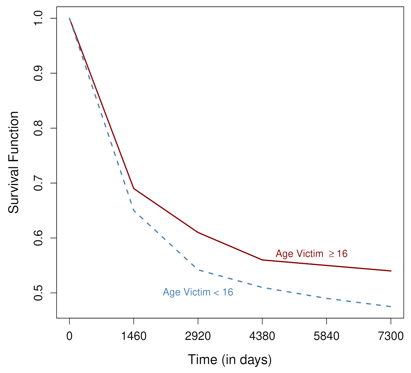
Four variables were significant with the Cox regression model: if the crimes committed by the individuals in 1973 were against persons under 16 years of age, the individuals tend to recidivate more rapidly. Higher rates of recidivism are observed among those that committed crimes against persons under the age of 16, as can be seen in Figure 1, in which the time axis is divided into four-year periods.
The results of the cure rate model give an estimated value of the parameter r of the Weibull distribution of , with a credibility interval at 95% of , indicating that the time distribution is not exponential. This translates into decreasing rather than constant risks. The estimations of the probability and temporal components of the cure rate model can be found in Table 1. It can be noted that the coefficient for the variable number of prior sexual crimes (NPS) has a credibility interval that contains zero, because of which we conclude that it does not contribute to explaining the probability of recidivism. The other variables show the same relationship as in the logistic regression: the number of prior non-sexual crimes increases the probability of recidivism, having committed the crime against a person under the age of 16 increases the probability of recidivism while being older decreases the probability of recidivism. The temporal component of the cure rate model only applies to those who repeat offences, because of which neither the number of prior sexual offences nor whether the victim was 16 and over or under 16 years of age in 1973 influences the risk of recidivism, given that both credibility intervals contain zero. In contrast, the risk of recidivism increases with the number of prior non-sexual crimes and decreases as age increases.
We present the global and by-group probabilities of recidivism in Table 2 at the end of the study and at three and ten years for the three models discussed in this article. The results are very similar.
It can be appreciated that 51.9% of the subjects had recidivated by the end of the follow-up. The logistic regression model gives the most approximate value of 52%, while the Cox regression model underestimated the rate by four percentage points and the cure rate model overestimated it by 0.7%. For the estimations of recidivism at ten years, which was 47.5%, the logistic and Cox regression models gave the best estimations, while the cure rate model overestimated the rate by 0.6%. At three years, the logistic and Cox regression models’ estimations were identical, but the cure rate model overestimated recidivism by 1.7%.
The real prevalence of recidivism at ten years was 33.1% among those who did not have prior convictions for sexual crimes. The three models over-estimated this value. The logistic regression is the closest with 2.8% of difference, followed by the cure rate model with 3.7% of difference and the Cox regression model with the largest difference with 6.9%. The recidivism rate for the group with five prior convictions for non-sexual crimes was much higher, at 89.9%, which was under-estimated by the three models. The cure rate model was the closest with 3.7% of difference, followed closely by the logistic regression model with 3.9% of difference, and finally, the Cox regression model over-estimated by 15.5%. The recidivism rate for the group of subjects without prior sexual crimes was 45.4%. The three models over-estimated by almost the same degree, the Cox regression model by 1.9%, the logistic regression model by 2%, and the cure rate model by 2.5%. The group’s recidivism rate with a prior conviction for a sexual crime was 66% at ten years. The cure rate model gave the best estimation with 0.5% over-estimation, while the logistic regression model over-estimated by 2.6% the Cox regression model over-estimated by double that at 5.3% of difference. For individuals under 25 years of age, the recidivism rate at ten years of follow-up was 59.1%. The closest value was that of the Cox regression model, which underestimated by 0.2%, followed the cure rate model closely with an underestimation of 0.4%, while the logistic regression model overestimated by 1.8%. The recidivism rate of individuals over 35 years of age was almost half that of individuals under 25, the youngest group. The three models underestimated the real value of 29.5% to similar degrees, 1.6%, 1.9%, and 2.3% by the logistic regression, cure rate, and Cox regression models. The recidivism rate at three years of the group without prior convictions for sexual crimes was 21.4%, which was overestimated by the three models. The closest was the cure rate model, with a difference of 1.1%, followed by the logistic regression model with 3.4% and the Cox regression model with 5%. Among subjects with prior convictions for non-sexual offences, the recidivism rate was 59.4% at three years. The Cox regression model underestimated this rate by 2.1% and the logistic regression and cure rate models by 3.8% and 4.2%, respectively. Among those who did not have prior non-sexual offences, 31.9% had recidivated at three years. The estimation of the cure rate model was 31.8%, while the Cox regression model overestimated by 1% and the logistic regression model by 1.4%. Some 46.7% of individuals with prior convictions for a sexual crime recidivated at three years. The three models underestimated the rate, the Cox regression model by 1.2%, the logistic regression model by 1.3%, and the cure rate model by 2.1%. Finally, the recidivism rate at three years among the youngest group, those under 25 years of age, was 44.1%, which was under-estimated by the three models. The closest is the logistic regression model with a difference of 2%, followed by the Cox regression model with a difference of 2.3%, while the cure rate model underestimated it by 4.3%. Recidivism at three years among those over 35 years of age was 17.8%. The Cox regression model gave an estimate of 17.7%, the logistic regression model with 1.9% less than the cure rate model underestimated it by 1.6%.
4.2. Prediction Models
In this section, we show non-linear survival methods’ ability to carry out recidivism predictions given the set of attributes of an individual. Unlike traditional methods like the linear Cox proportional hazards model, non-linear models can deal with high interaction terms. Therefore, they can offer interesting performances for prediction activities.
For DeepSurv training and predictions, the Python (version 3.7, Python Software Foundation, https://www.python.org/ accessed on 23 January 2021) module of the same name was used. CPH and RSF training and predictions were carried out with the modules in Python lifelines and RandomForestClassifier, respectively.
The variables NP (number of previous nonsexual convictions in the past ten years), NPS (number of previous sexual convictions in the past ten years), AGE (age of offender) the and Av_u16 (if the aged victim was under 16 years old) were used as predictors. The dataset with 3068 instances was divided into a disjointed set of training (80%) and testing (20%), the latter to estimate the models’ performance. The process of dividing the sample in this way was carried out 100 different times so that 100 different models were estimated for DeepSurv, CPH, and RSF.
The continuous input variables to the neural network were previously standardized (NP, NPS, and AGE). As an optimal activation layer, the ReLU was chosen (Nair and Hinton, 2010). The hyper-parameters of the network—number of hidden layers, number of nodes on each layer, batch size, drop-rate, and learning rate—were determined on a grid search for different values of each parameter and choosing the one that grants the maximum performance measured in the concordance index. Adding more than four hidden layers to the neural network did not show improvements in predictive performance, so it was left in 4 layers with 256 nodes in each. To prevent overfitting, the dropout probability between hidden layers was 10% [32], with a learning rate of 0.004, batch size of 256, and an Adam optimizer used for model training.
The performance measure used to evaluate and compare the three models was the concordance index, which measures the agreement between the predicted risks and actual survival [29]. This measure is calculated for the training and testing datasets, both of which are mutually exclusive in each of the simulations. The concordance index is used as a performance measure for the prediction of survivorship. It has the advantage of not depending on a simple fixed time measure for evaluation and also considers the censoring nature of the dataset [3].
Table 3 shows the concordance index results over the 100 simulations in each of the three models. The results show that DeepSurv is superior to CPH and RSF in both the training and test sets. This result can be considered as a sign that DeepSurv correctly learns the non-linear relationships between the covariates of repeaters and their log-risk [4]. The performance between CPH and RSF performance is very similar, at least in the test set. Even these results are consistent with different simulations of 100 runs.
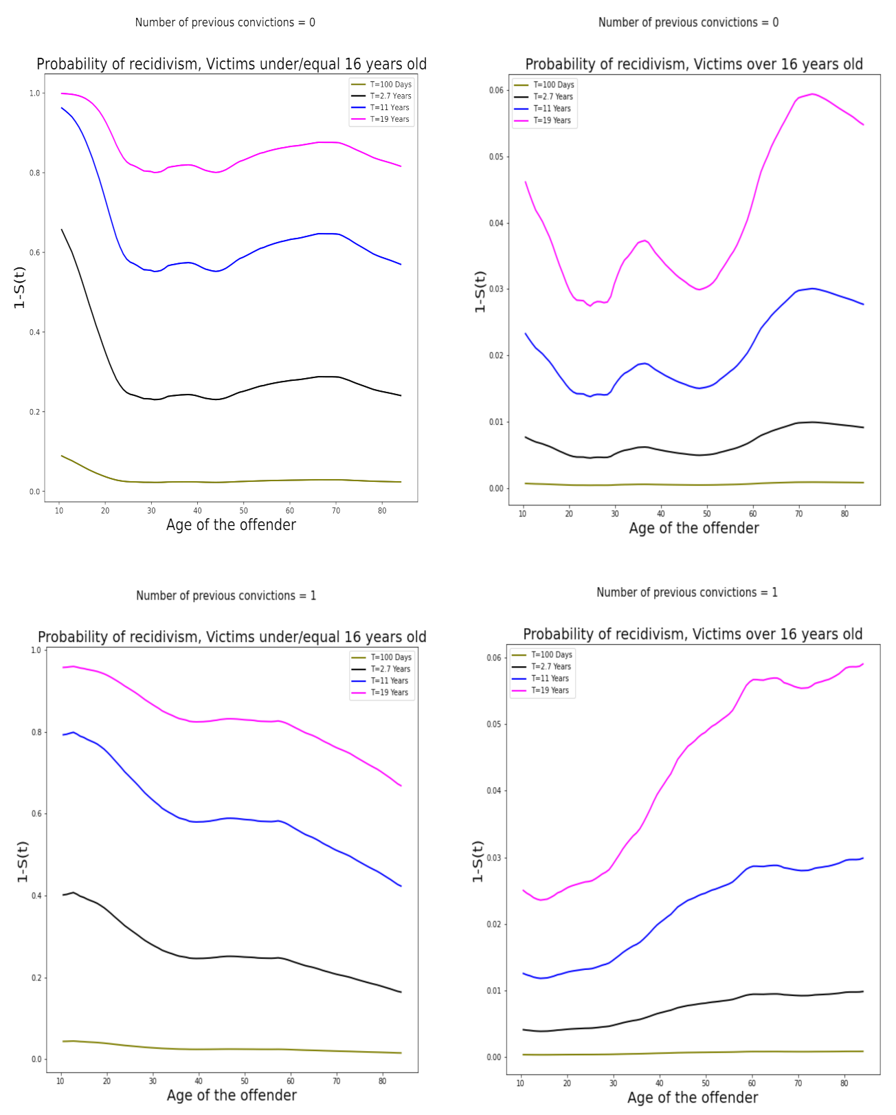
To complement the result of the predictions with the neural network, Figure 2 shows the offenders’ recidivism probabilities at certain moments. As indicated before, for a given set of attributes, DeepSurv delivers a predicted log-risk score, which is used to lead to an estimate of the survival function . Thus, the offender recidivism probability will be . After neural network training, we select four-time instants (T = 100 days, T = 2.7, T = 11, and T = 19 years) and a particular value of attributes. For example, we see that recidivism probabilities have very different behavior, depending on whether the victims of the offences are older than 16 years old versus when they are younger or equal to that age. It is clear that these probabilities are very low when the victim was over 16, but with younger victims, the probability is higher than 0.5 after 2.7 years. Different behavior is also observed according to the number of previous convictions. For example, in extreme cases when the number of previous convictions was one for each type of conviction (one nonsexual and one sexual conviction in the past ten years), we see that as the age of the offender increases, the probability of recidivism decreases slightly when the victim was under or equal to 16 years of age, but not when she is over 16 years of age. These examples show the usefulness of this type of model from which it is possible to answer questions in the style of what if and eventually take preventive measures.
5. Conclusions
Among the statistical explaining models, we can conclude that there is no predominance of one model as better than the others in any of these situations. In the original work [16], a more complex group of models is fitted, which we referred to above as competitive risk models, which are an extension of the cure rate models presented in this workwhen it is of interest to model specific recidivism rates—that is, the recidivism rate for a type of crime.
We have applied the Weibull distribution, the distribution function of which has an explicit form. This is not always the case. When the distribution function of the time until recidivating is not closed, there is difficulty in fitting these models from the Bayesian point of view. This is the case if the distribution is gamma or lognormal. We also implemented some of these models using JAGS, which will be the focus of future works.
In previous studies with a completely different data domain (e.g., cancer prevention [33] and biomedical applications [2,34]), it has been found that neural networks, and, in particular, the multilayer perceptron, have been superior in performing predictive activities in survival analysis. In this work, the results did not differ much. Our results are in the same line as those of [35], in which they showed the predictive superiority of neuronal networks over logistic regression models in the problem of prediction of criminal recidivism. Deep learning applied to recidivism data proves to be superior to the linear Cox proportional hazards model and even better than random survival forests. This highlights the versatility of deep neural networks to deal with different data domains in survival analysis.
We believe that there is potential for this type of tool to be a valid option for crime and recidivism prevention. The development of risk assessment scales to determine risk groups can help us make decisions regarding the prevention of criminal behavior recidivism [36]. In this case, the neural network can continuously assess risk in the light of new information for a given instance. In this sense, a new and updated database of recidivism activities could regularly feed these models, which could benefit not only society but also those at high risk of committing a crime.
While the learning machines such as DeepSurv used in this study perform acceptably in prediction activities, it is also true that these types of models become more opaque or less transparent compared to statistical models where there is greater clarity in how the predictors relate to the output. As seen in this work, the evaluation of recidivism analysis is more transparent in classical models for censored data.
In line with the above, it would now be advisable for interpretability purposes, [37] to perform the constant revision and estimation of statistical models that allow the analyst, together with well-performing predictive models, to have the cross-validation of models, especially for applications in which it is necessary to carry out diagnostics and evaluate risk scales.
Author Contributions
Conceptualization, R.d.l.C., O.P., M.A.V. and G.A.R.; methodology, R.d.l.C., O.P., M.A.V. and G.A.R.; software, R.d.l.C., O.P. and M.A.V.; validation, R.d.l.C. and M.A.V.; formal analysis, R.d.l.C., O.P., M.A.V. and G.A.R.; investigation, R.d.l.C., O.P., M.A.V. and G.A.R.; resources, R.d.l.C. and G.A.R.; data curation, R.d.l.C.; writing—original draft preparation, R.d.l.C., O.P. and M.A.V.; writing—review and editing, R.d.l.C., M.A.V. and G.A.R.; visualization, R.d.l.C. and M.A.V.; supervision, R.d.l.C. and G.A.R.; project administration, R.d.l.C.; funding acquisition, R.d.l.C. and G.A.R. All authors have read and agreed to the published version of the manuscript.
Funding
This research was funded by ANID FONDECYT grant number 1181662, and ANID FONDECYT grant number 1180706.
Institutional Review Board Statement
Not applicable.
Informed Consent Statement
Not applicable.
Data Availability Statement
The data presented in this study are available on request from the corresponding author.
Acknowledgments
The authors are grateful to Gabriel Escarela for providing the dataset used in the experiments.
Conflicts of Interest
The authors declare no conflict of interest.
References
- Ross, S.; Guarnieri, T. Recidivism Rates in a Custodial Population: The Influence of Criminal History, Offence & Gender Factors. Available online: https://citeseerx.ist.psu.edu/viewdoc/summary?doi=10.1.1.421.3985&rank=1 (accessed on 11 November 2020).
- Gensheimer, M.F.; Narasimhan, B. A scalable discrete-time survival model for neural networks. PeerJ 2019, 7, e6257. [Google Scholar] [CrossRef] [PubMed]
- Kim, D.W.; Lee, S.; Kwon, S.; Nam, W.; Cha, I.H.; Kim, H.J. Deep learning-based survival prediction of oral cancer patients. Sci. Rep. 2019, 9, 1–10. [Google Scholar] [CrossRef] [Green Version]
- Katzman, J.L.; Shaham, U.; Cloninger, A.; Bates, J.; Jiang, T.; Kluger, Y. DeepSurv: Personalized treatment recommender system using a Cox proportional hazards deep neural network. BMC Med. Res. Methodol. 2008, 18, 24. [Google Scholar] [CrossRef] [PubMed]
- Hoffman, P.B.; Stone-Meierhoefer, B. Reporting recidivism rates: The criterion and follow-up issues. J. Crim. Justice 1980, 8, 53–60. [Google Scholar] [CrossRef]
- Beck, A.J.; Shipley, B.E. Recidivism of Prisoners Released in 1983. Available online: https://www.bjs.gov/content/pub/pdf/rpr83.pdf (accessed on 17 June 2020).
- Gendreau, P.; Little, T.; Goggin, C. A Meta-analysis of the predictors of adult offender recidivism: What works! Criminology 1996, 34, 575–608. [Google Scholar] [CrossRef]
- Piquero, A.R. Assessing the relationships between gender, chronicity, seriousness, and offense skewness in criminal offending. J. Crim. Justice 2000, 28, 103–115. [Google Scholar] [CrossRef]
- Andrews, D.A. Recidivism is predictable and can be influenced: Using risk assessment to reduce recidivism. IARCA 1989, 1, 11–17. [Google Scholar]
- Hanson, R.K.; Bussiere, M.T. Predicting relapse: A meta-analysis of sexual offender recidivism studies. J. Consult. Clin. Psychol. 1998, 66, 348–362. [Google Scholar] [CrossRef]
- Schmidt, P.; Dryden, W.A. Predicting Criminal Recidivism using ‘Split Population’ Survival Time Models. J. Econom. 1989, 40, 141–159. [Google Scholar] [CrossRef] [Green Version]
- Barton, R.R.; Turnbull, B.W. A failure rate regression model for the study of recidivism. In Models in Quantitative Criminology; Fox, J.A., Ed.; Academic Press: New York, NY, USA, 1981. [Google Scholar]
- Schell, T.L.; Chan, K.S.; Morral, A.R. Predicting DUI recidivism: Personality, attitudinal, and behavioral risk factors. Drug Alcohol Depend. 2006, 82, 33–40. [Google Scholar] [CrossRef]
- Bierens, H.J.; Carvalho, J.R. Semi-Nonparametric Competing Risks Analysis of Recidivism. J. Appl. Econ. 2007, 22, 971–993. [Google Scholar] [CrossRef] [Green Version]
- Padilla, O.; De la Cruz, R. Bayesian split-population models for estimating recidivism. Chil. J. Stat. 2021, in press. [Google Scholar]
- Escarela, G.; Francis, B.; Soothill, K. Competing Risks, Persistence, and Desistance in Analyzing Recidivism. J. Quant. Criminol. 2000, 16, 385–414. [Google Scholar] [CrossRef]
- Hosmer, D.; Lemeshow, S. Applied Logistic Regression, 2nd ed.; John Wiley & Sons: New York, NY, USA, 2000. [Google Scholar]
- Marshall, G.; Shroyer, A.L.W.; Grover, F.L.; Hammermeister, K.E. Bayesian-logit model for risk assessment in coronary artery bypass grafting. Ann. Thorac. Surg. 1994, 57, 1492–1500. [Google Scholar] [CrossRef]
- Ntzoufras, I. Bayesian Modeling Using Winbugs, 1st ed.; John Wiley & Sons: New York, NY, USA, 2011. [Google Scholar]
- Congdon, P. Applied Bayesian Modelling, 2nd ed.; John Wiley & Sons: New York, NY, USA, 2014. [Google Scholar]
- Maller, R.; Zhou, X.S. Survival Analysis with Long—Term Survivors; John Wiley & Sons: New York, NY, USA, 1996. [Google Scholar]
- Ibrahim, J.G.; Chen, M.H.; Sinha, D. Bayesian Survival Analysis; Springer: New York, NY, USA, 2005. [Google Scholar]
- Martin, A.; Kevin, M.; Quinn, K.; Hee-Park, J. Markov Chain Monte Carlo in R. J. Stat. Softw. 2011, 42, 1–22. [Google Scholar] [CrossRef] [Green Version]
- Raftery, A.; Hoeting, J.; Volinsky, C.; Painter, I.; Yee Yeung, K. BMA: Package for Bayesian Model Averaging and Variable Selection for Linear Models, Generalized Linear Models and Survival Models. R Package Version 3.18.14. Available online: https://cran.r-project.org/web/packages/BMA/BMA.pdf (accessed on 23 January 2021).
- Plummer, M. rjags: Bayesian Graphical Models Using MCMC. R Package Version 3-10. Available online: https://cran.r-project.org/web/packages/rjags/rjags.pdf (accessed on 23 January 2021).
- Faraggi, D.; Simon, R. A neural network model for survival data. Stat. Med. 1995, 14, 73–82. [Google Scholar] [CrossRef]
- Xiang, A.; Lapuerta, P.; Ryutov, A.; Buckley, J.; Azen, S. Comparison of the performance of neural network methods and Cox regression for censored survival data. Comput. Stat. Data Anal. 2001, 34, 243–257. [Google Scholar] [CrossRef]
- Sargent, D.J. Comparison of artificial neural networks with other statistical approaches. Cancer 2001, 91, 1636–1642. [Google Scholar] [CrossRef]
- Harrell, F.E.; Califf, R.M.; Pryor, D.B.; Lee, K.L.; Rosati, R.A. Evaluating the yield of medical tests. JAMA 1982, 247, 2543–2546. [Google Scholar] [CrossRef]
- Ishwaran, H.; Kogalur, U.B.; Blackstone, E.H.; Lauer, M.S. Random survival forests. Ann. Appl. Stat. 2008, 2, 841–860. [Google Scholar] [CrossRef]
- Breiman, L. Random forests. Mach. Learn. 2001, 45, 5–32. [Google Scholar] [CrossRef] [Green Version]
- Srivastava, N.; Hinton, G.; Krizhevsky, A.; Sutskever, I.; Salakhutdinov, R. Dropout: A simple way to prevent neural networks from overfitting. J. Mach. Learn. Res. 2018, 15, 1929–1958. [Google Scholar]
- Huang, Z.; Johnson, T.S.; Han, Z.; Helm, B.; Cao, S.; Zhang, C.; Salama, P.; Rizkalla, M.; Yu, C.Y.; Cheng, J.; et al. Deep learning-based cancer survival prognosis from RNA-seq data: Approaches and evaluations. BMC Med. Genom. 2020, 13, 41. [Google Scholar] [CrossRef] [PubMed] [Green Version]
- Street, W.N. A Neural Network Model for Prognostic Prediction. In Proceedings of the International Conference on Machine Learning (ICML), Madison, WI, USA, 24–27 July 1998; pp. 540–546. [Google Scholar]
- Palocsay, S.W.; Wang, P.; Brookshire, R.G. Predicting criminal recidivism using neural networks. Socio-Econ. Plan. Sci. 2000, 34, 271–284. [Google Scholar] [CrossRef]
- Tollenaar, N.; Van Der Heijden, P.G. Optimizing predictive performance of criminal recidivism models using registration data with binary and survival outcome. PLoS ONE 2019, 14, e0213245. [Google Scholar] [CrossRef] [PubMed] [Green Version]
- Freitas, A.A. Comprehensible classification models: A position paper. ACM SIGKDD Explor. Newsl. 2014, 15, 1–10. [Google Scholar] [CrossRef]
Figure 1.
Dependence of the survival function of the age of the victim.

Figure 2.
DeepSurv predictions of recidivism probability in different periods, for different ages and previous convictions.
Figure 2.
DeepSurv predictions of recidivism probability in different periods, for different ages and previous convictions.


Table 1.
Estimation of the probability and temporal components of recidivism in the cure rate model.
Table 1.
Estimation of the probability and temporal components of recidivism in the cure rate model.
| Variable | Parameter | 95% Credible Interval | ||
|---|---|---|---|---|
| Probability of Recidivism | Intercept | 0.573 | 0.357 | 0.794 |
| NP | 0.532 | 0.459 | 0.611 | |
| NPS | 0.167 | −0.064 | 0.416 | |
| AGE | −0.405 | −0.466 | −0.344 | |
| Av_u16 | 0.314 | 0.135 | 0.493 | |
| Temporal | Intercept | 0.665 | −1.079 | 2.434 |
| NP | 1.097 | 0.867 | 1.318 | |
| NPS | −0.786 | −1.842 | 0.147 | |
| AGE | −1.614 | −2.251 | −1.015 | |
| Av_u16 | 0.061 | −1.189 | 1.345 | |
Table 2.
Percentages of global and by-group recidivism for the logistic regression, Cox, and Cure rate models at 3 and 10 years.
Table 2.
Percentages of global and by-group recidivism for the logistic regression, Cox, and Cure rate models at 3 and 10 years.
| Real | Logistic Regression | Cox Regression Model | Cure Rate Model (Weibull) | |
|---|---|---|---|---|
| Recidivism general | 51.9 | 52 | 47.8 | 52.6 |
| Recidivism at 10 years | 47.5 | 47.3 | 47.7 | 48.1 |
| Recidivism at 3 years | 33.4 | 33.3 | 33.3 | 31.7 |
| Recidivism by groups at 10 years | ||||
| NP = 0 | 33.1 | 35.9 | 40 | 36.8 |
| NP = 5 | 89.9 | 86 | 74.4 | 86.2 |
| NPS = 0 | 45.4 | 47.4 | 47.3 | 47.9 |
| NPS > 0 | 66 | 63.4 | 60.7 | 66.5 |
| AGE < 25 | 59.1 | 57.3 | 58.9 | 58.7 |
| AGE > 35 | 29.5 | 27.9 | 27.2 | 27.6 |
| Recidivism by groups at 3 years | ||||
| NP = 0 | 21.4 | 24.8 | 26.4 | 22.5 |
| NP = 5 | 59.4 | 63.2 | 57.3 | 63.6 |
| NPS = 0 | 31.9 | 33.3 | 32.9 | 31.8 |
| NPS > 0 | 46.7 | 45.4 | 45.5 | 44.6 |
| AGE < 25 | 44.1 | 42.1 | 41.8 | 39.8 |
| AGE > 35 | 17.8 | 16.9 | 17.7 | 16.2 |
Table 3.
Results of the concordance index (95% confidence interval) for all experiments.
| Model | Train Set | Test Set |
|---|---|---|
| CPH | 0.696 (0.690, 0.701) | 0.693 (0.669, 0.716) |
| RSF | 0.749 (0.745, 0.754) | 0.687 (0.665, 0.708) |
| DeepSurv | 0.800 (0.793, 0.806) | 0.789 (0.774, 0.800) |
Publisher’s Note: MDPI stays neutral with regard to jurisdictional claims in published maps and institutional affiliations. |
© 2021 by the authors. Licensee MDPI, Basel, Switzerland. This article is an open access article distributed under the terms and conditions of the Creative Commons Attribution (CC BY) license (http://creativecommons.org/licenses/by/4.0/).
Share and Cite
MDPI and ACS Style
de la Cruz, R.; Padilla, O.; Valle, M.A.; Ruz, G.A. Modeling Recidivism through Bayesian Regression Models and Deep Neural Networks. Mathematics 2021, 9, 639. https://doi.org/10.3390/math9060639
AMA Style
de la Cruz R, Padilla O, Valle MA, Ruz GA. Modeling Recidivism through Bayesian Regression Models and Deep Neural Networks. Mathematics. 2021; 9(6):639. https://doi.org/10.3390/math9060639
Chicago/Turabian Stylede la Cruz, Rolando, Oslando Padilla, Mauricio A. Valle, and Gonzalo A. Ruz. 2021. "Modeling Recidivism through Bayesian Regression Models and Deep Neural Networks" Mathematics 9, no. 6: 639. https://doi.org/10.3390/math9060639
Note that from the first issue of 2016, this journal uses article numbers instead of page numbers. See further details here.