
Abstract
The use of microfluidic devices in the field of plasma-liquid interaction can unlock unique possibilities to investigate the effects of plasma-generated reactive species for environmental and biomedical applications. So far, very little simulation work has been performed on microfluidic devices in contact with a plasma source. We report on the modelling and computational simulation of physical and chemical processes taking place in a novel plasma-microfluidic platform. The main production and transport pathways of reactive species both in plasma and liquid are modelled by a novel modelling approach that combines 0D chemical kinetics and 2D transport mechanisms. This combined approach, applicable to systems where the transport of chemical species occurs in unidirectional flows at high Péclet numbers, decreases calculation times considerably compared to regular 2D simulations. It takes advantage of the low computational time of the 0D reaction models while providing spatial information through multiple plug-flow simulations to yield a quasi-2D model. The gas and liquid flow profiles are simulated entirely in 2D, together with the chemical reactions and transport of key chemical species. The model correctly predicts increased transport of hydrogen peroxide into the liquid when the microfluidic opening is placed inside the plasma effluent region, as opposed to inside the plasma region itself. Furthermore, the modelled hydrogen peroxide production and transport in the microfluidic liquid differs by less than 50% compared with experimental results. To explain this discrepancy, the limits of the 0D–2D combined approach are discussed.
Export citation and abstract BibTeX RIS

Original content from this work may be used under the terms of the Creative Commons Attribution 4.0 license. Any further distribution of this work must maintain attribution to the author(s) and the title of the work, journal citation and DOI.
1. Introduction
We recently reported on our development of a platform that combines a non-thermal atmospheric pressure plasma source and a microfluidic device [1]. It offers the possibility to connect different plasma source types with different microfluidic chips, and provides a novel tool for studying plasma-liquid interactions with high spatial resolution and in situ chemical analysis. Furthermore, it sets the basis to the coupling of a reference biomedical plasma source with well-established biological models embedded in microfluidic devices. In the current article we present a computational modelling approach to improve our understanding of the main production and transport pathways of plasma-generated reactive species in the plasma volume and in its effluent, and in the contacting liquid for a geometrically simplified version of the experimental setup.
Existing plasma-microfluidic technologies include non-thermal plasma (NTP) inside microchannels [2, 3], microfluidic plasma arrays [4] and NTP sources directly embedded inside microfluidic devices [5–7]. Key plasma-microfluidic research has been reviewed by Lin et al [8]. In our previous work [1], we introduced a plasma-microfluidic platform with unique design criteria, including the liquid flow inside the microfluidic device, the formation of a stable plasma-liquid interaction zone and in situ optical access. This was achieved by creating a multiphase gas-liquid flow where small volumes of water are brought in direct contact with the plasma or effluent of the plasma source. In our case, the plasma source is based on the COST reference plasma jet which was designed to provide the low-temperature plasma community a reference plasma source with easy diagnostic and modelling access. Today, it is used by numerous research groups and both experimental and modelling data are widely available [9]. Different approaches have been used to model the physical and chemical processes taking place inside the COST-jet's plasma-forming region and effluent. To model the chemical kinetics, zero-dimensional (0D) modelling is the most common approach [10–13]. Here, complex plasma processes and extensive reaction sets can be accounted for with relatively low computational times [14]. The obvious drawback of this approach is the absence of spatial information [15]. However, using the average plasma-forming gas velocity in the plasma channel does allow coupling of the time variation (as calculated in a 0D kinetic model) to the distance variation, providing a quasi-1D plug flow model [16]. Multidimensional plasma simulations are demanding in terms of computational resources and require significant simplifications and approximations to achieve reasonable computation times. In the realm of computational studies of the COST-jet, these simplifications include the use of a multi-time scale approach [17], the combination of more than one modelling approach (hybrid technique) [18] and/or a limited chemical reaction set [19, 20].
For the study of our plasma-microfluidic platform, plasma-liquid interactions also are of high interest. Plasma-liquid interactions have been increasingly studied in recent years [21]. With a simplified 2D axisymmetric model, Lindsay et al studied the interaction between a pulsed streamer discharge and a liquid-filled vessel in terms of fluid dynamics, heat transfer and reaction mechanisms of key chemical species, both in the gas and liquid phases [22]. The number of species included in this model was limited and no electron impact reactions were considered for faster computation. Heffny et al used a fluid dynamic model to simulate the COST-jet above liquid water, although the water phase itself was not modelled. They fixed the concentration of reactive species at the exit of the COST-jet based on experimental results [19]. Mohades et al used a 2D model to study the interaction between a helium plasma jet and water in a well plate, but the simulation results could not be compared to experimental work [23]. Verlackt et al used 2D modelling to study the chemistry and plasma-liquid interactions of an argon plasma jet, the kINPen®, above a liquid sample [24]. Heirman et al further improved this model by combining 0D reaction kinetics with 2D reaction-diffusion-convection to model the kINPen above a well of a 12 well-plate and compared the results to experimental liquid diagnostics of key reactive species [14]. The latter works were all for plasma jets interacting with large volumes of liquid (more than 1 ml). The plasma treatment of small liquid volumes, such as water droplets, was also modelled by Oinuma et al [25], Kruszelnicki et al [26] and Lai and Foster [27]. However, to the best of our knowledge, no modelling work has been conducted to study the interaction between small volumes of liquid and the COST-jet plasma channel, and compared with experimental work. Our plasma-microfluidic platform offers ideal conditions for such studies.
We report on the implementation of a computational model to study the plasma-generated chemistry and species transport inside the plasma-microfluidic platform. The model takes advantage of the highly unidirectional flow inside the COST-jet to model the reaction kinetics with a 0D plug flow model approach while retaining 2D spatial information. This is achieved by using both ZDPlaskin [28] and COMSOL Multiphysics [29]. The simulation approach combining 0D and 2D modelling, based on the approach presented by Heirman et al [14], is introduced together with the results it provides in terms of key reactive species. These results are compared to experimental work and the limitations of the model are discussed.
2. Model overview
The plasma source we chose for our plasma-microfluidic platform is based on the COST reference plasma jet [2], which consists of a continuous wave capacitively-coupled radiofrequency (13.56 MHz) plasma jet. Helium with small admixture of water vapour (4500 ppm) is the plasma-forming feed gas of the  mm3 plasma channel. Our plasma-microfluidic device, presented elsewhere [1], is modelled as a channel divided into two regions: a 30 mm-long plasma-forming region with a
  mm2 cross-section followed by a plasma effluent (afterglow) region of the same dimensions (figure 1). This plasma and effluent channel is put in contact with a small water volume of
  mm3, which represents the water segments flowing in the microfluidic device. The gas-liquid interface can be placed at any location in the channel, both under the plasma active zone or under the plasma effluent. The free liquid surface is separated from the plasma or effluent channel by a gap of 0.1 mm where no plasma reaction kinetics are directly solved. Additional information on the modelling of this gap will be provided in sections 5 and 6. Figure 1 shows the schematics of the computational model geometry for a plasma-liquid interaction zone positioned (a) under the plasma active zone and (b) under the plasma effluent. The modelled system's geometry is a cross-section of the 3D geometry expanding out of the plane.
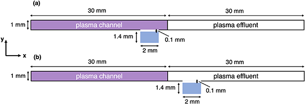
Figure 1. Schematic of the geometry used for the simulation model. (a) The liquid volume is placed under the active plasma zone. (b) The liquid is placed under the plasma effluent.
Download figure:
Standard image High-resolution imageFigure 2 shows a flowchart representation of the computational model. The modelling approach is based on the computational scheme presented in [14]. The blue coloured steps are described in detail in the respective sections of the article. Our approach uses a combination of multiple 0D simulations of the plasma chemistry with ZDPlaskin and 2D simulations computed with COMSOL Multiphysics (version 6.0). This approach is used to reduce computing time. Since the simulated chemistry inside the plasma active zone consists of over 1000 reactions, as will be discussed in section 4, full 2D or 3D simulations would be too computationally intensive to solve within a reasonable time. Moreover, many of the reactions are electron impact reactions. For these reactions, the Boltzmann equation must be solved to find the reaction rates. Combining both 0D and 2D modelling sequentially leverages the advantages of both, solving complex chemistry in a reasonable computational time while keeping dimensional transport information.

Download figure:
Standard image High-resolution imageThe first step (I) is to simulate the humidified helium flow inside the channel in 2D. This step provides spatially-resolved information on the gas velocity and temperature, and water vapour distribution in the channel. This information is needed for the 0D-plug flow plasma chemistry model of step II. In this second step, the channel is broken down into thinner domains, which we will further refer to as 'bins', as shown in figure 3. In our approach, each bin is modelled as an independent plug flow system for which the plasma reaction kinetics is solved. For each bin, a different temperature and water vapour concentration profile, provided by the 2D humidified helium flow simulation (step I), is applied to solve the corresponding chemistry with a 0D-plug flow model. This approach neglects the effect of species diffusion in the direction perpendicular to the gas flow (crosswind diffusion) on the reaction kinetics. This approximation is justified by the high Péclet (Pe) number defined as  where
where  is the bulk velocity,
  the characteristic length and
  the diffusion coefficient. As will be presented later, the results of this first 2D model show that the gas flow in the channel has a bulk velocity of 25 m s −1 (Reynold number, Re
 ). The diffusion coefficients of the plasma-generated species are typically on the other of
  m2 s−1. Assuming a characteristic length of
  mm (average width of the bins), we obtain
  This high value justifies dividing the domain in bins; the transport through convection in the direction of the gas flow is higher than the transport through diffusion in the crosswind direction.
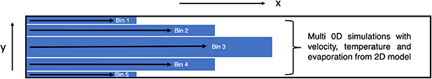
Figure 3. The channel is separated in different bins. The chemical kinetics of each bin is solved by a different 0D model with different parameters, such as gas velocity, gas temperature and water vapour concentration concentration. For simplicity only 5 bins are illustrated while for the model, 11 bins are used.
Download figure:
Standard image High-resolution imageThe results of the reaction kinetics of each bin are then used in step III as inputs to a second two-dimensional COMSOL model which considers a limited number of plasma-generated species. This 2D model additionally considers the transport of plasma-generated species to the liquid phase along with the reaction kinetics inside the liquid.
In the following sections, each step of the simulation procedure is discussed in further details. Figure 2 summarizes the computational approach:
- I.A 2D model simulates the plasma and effluent channel, without solving for any chemistry, to provide spatially-resolved information on gas velocity, gas temperature and water vapour concentration (humidity). (Section 3)
- II.The simulation domain is split in thin bins. The chemistry and reactive species evolution in each bin is solved independently in a 0D-plug flow model using the results provided by the first 2D model. (Section 4)
- III.A second 2D model uses the results of each bin's plug flow simulation to model the evolution of plasma reactive species in two dimensions in the plasma channel, effluent channel and inside the liquid. (Section 5)
3. Step I: 2D model for velocity, temperature and water vapour concentration
The first 2D model solves for the gas velocity, gas temperature and water vapour concentration in the channel. The steady state velocity distribution is computed by solving the Navier-Stokes equation for an incompressible and Newtonian fluid, and the continuity equation:

where  is the mass density in kg m−3,
  is the velocity field in m s−1,
  is the pressure in Pa, and
  is the dynamic viscosity in Pa
 s. A flow rate of 1.5 slm is used at the inlet. The outlet pressure is fixed at atmospheric pressure while all other boundaries exhibit zero velocity (no-slip condition). The computed velocity profile is then used as input for a second simulation which calculates heat and species transport. The temperature profile is found by solving the time-dependent energy equation:
where  is the specific heat capacity in J kg−1·K,
  is the temperature in K,
  is the thermal conductivity in W m−1·K, and
  is the net volumetric heat source due to plasma (Joule) heating and water evaporation, in W m−3. The temperature at the inlet is fixed. In the plasma-forming region of the channel a constant volumetric heat source is considered; the plasma power dissipation (typically 1 W) divided by the plasma volume (30
  1
1  1 mm3). Hence, we assume in our heat transfer simulation that all the energy consumed by the plasma is dissipated as heat. This approximation deliberately neglects the energy losses through photon emission, species excitation and species ionization. Nonetheless, this simplification is supported by previous findings, including [12, 30], which have demonstrated that a significant proportion of the plasma's energy in the COST-Jet is dissipated as heat. Additionally the temperature profile obtained from our simulations using this approximation aligns with experimental observation [30], justifying its applicability in our model.
An interfacial heat flux is considered at the gas-liquid interface resulting from the evaporation of water:

where  is the heat flux at the gas-liquid interface in W m−2,
  is the water vapour flux at the interface perpendicular to the latter in kg m−2·s and
  is the latent heat of evaporation of water in J kg−1. All other boundaries, except for the outlet, are thermally insulated.
The water vapour concentration along the plasma and effluent channel originates from the evaporation at the gas-liquid interface. It is found with the species conservation equation:
where  is the water concentration in mol m−3 and
  is the diffusivity of water vapour in helium, in m2 s−1. The gas inlet has a humidity fixed at a concentration matching the experimental conditions (4500 ppm). The water vapour concentration at the gas-liquid interface is kept at 100% relative humidity, the corresponding water vapour concentration given by Antoine's Law [31]. No humidity flux is considered at the other boundaries except for the outlet. The convective transport of water vapour is computed with the solution of the laminar flow module, while the diffusion of water vapour in helium is calculated with the mass diffusivity of
  in helium (see section 5.1).
4. Step II: 0D model for reactive species production
The 0D simulations are performed using ZDPlaskin [28], a freeware that solves a set of conservation equations (one for each species) based on production and loss rates as defined by chemical reactions:
 is the density of species s,
  is the number of reactions,
  and
and  are the stoichiometric coefficients of species
  in reaction
  on the right side and left side of the reaction, respectively,
  is the reaction rate coefficient of the
  reaction and
  is the density of the
  reactant of reaction
  elevated to the power equal to its stoichiometric coefficient
  [28].
[28].
To evaluate reactive species production, we employed the chemical reaction set constructed by Aghaei and Bogaerts [32] specifically for He in contact with N2, O2 and H2O. We considered 90 chemical species (plus electrons). The chemistry set describes 1437 reactions, including 148 electron impact reactions, 71 electron–ion recombination reactions, 412 ion–ion reactions, 399 ion–neutral reactions, and 407 neutral reactions, as described in [32]. The reaction rate coefficients of heavy species (other than electron impact) reactions are either constant or gas-temperature dependent. The reaction rate coefficients of electron impact reactions are calculated using:
where  is the threshold energy of the reaction,
  is the cross-section of collision
  ,
,  is the electron velocity and
  is the electron energy distribution function (EEDF). The electron impact reactions are hence dependent on the electron energy. The EEDF is found by solving the Boltzmann equation with the built-in solver BOLSIG +. To do so, the Boltzmann solver uses a set of electron impact cross-sections, the gas temperature, reduced electric field and electron density. The reduced electric field in V m−1 is kept constant at a value given by the local-field approximation [33]:

where  is the plasma power density in W m−3, and
  is the plasma conductivity in S m−1 calculated with:

where  is the elementary charge in C,
  is the electron drift velocity in m s−1,
  is the electron density in 1 m−3 and
  is the electric field in V m−1 at the previous time step.
The main parameters that influence the reaction kinetics evolution, such as temperature and water vapour concentration, vary spatially in the plasma and effluent channel. To consider these variations, the results from the 2D humidified helium gas flow simulation are used. The average velocity of each bin is used in the corresponding plug flow simulation. The plasma-forming gas velocity enables the coupling between time and distance in each plug flow model. For each bin, the temperature along the x-axis (plug flow axis) from the previous 2D model is implemented in the corresponding simulation. As each bin is not infinitely thin, the y-averaged values are used along the x-axis. The concentration of water vapour is introduced slightly differently than the temperature in the 0D simulations. Since the reaction kinetics influence the concentration of  along the x-axis, the concentration of
  cannot be fixed (as was done for the temperature). Instead, the model considers the variation of
  concentration along the plug flow axis. This variation arises from the mixing of the evaporated water at the gas-liquid interface with the humidified helium. To account for it, the spatial derivative of the
  concentration along the x-axis is used to feed the different 0D plug flow models.
For the results presented in this work, the plasma and effluent channel is split into 11 bins (note that in figure 3 only 5 bins are illustrated for simplicity). Each bin has a length (dimension along the x-axis) of 60 mm: 30 mm of plasma and 30 mm of effluent. The four outermost bins (2 at the upper and 2 at the lower edge) are 50 μm-wide (dimension along the y-axis), the central bin is 200 μm-wide and the remaining bins are 100 μm-wide. For each of these 11 bins, one independent 0D plug flow simulation is performed.
5. Step III: 2D plasma-generated species transport model
5.1. Transport of species in the plasma channel and effluent channel
In the plasma and effluent channel, the concentration of each reactive species of interest is solved for in 2D using the species conservation equation:
where  is the concentration of species
  ,
,  is the diffusivity in helium of species
  ,
,  is the velocity vector field solved as presented in section 3, and
  is the source term of species
  in mol (m3s)−1. The diffusivity of each species,
  , in helium is calculated using the Chapman–Enskog theory [34]:
where D is the diffusivity in m2 s−1, A is an empirical constant equal to  ,
,  is the temperature in K,
  and
and  are the molar masses of helium and the species of interest, respectively.
  is the pressure in Pa and
  is the temperature-dependent collision integral given by [34]:
where 
 ,
,  ,
,  and
and  are the Lennard-Jones parameters of helium and the species of interest. The temperature profile obtained from the humidified helium gas flow 2D model (discussed in section 3) is used to calculate the diffusivities. Table 1 presents the Lennard-Jones parameters for the species of interest used in the model.
Table 1. Lennard-Jones parameters of gas species. For HNO, the values of HO2 were used because no information was available in literature.
| Species | σ (m) |
 (J) (J) | References |
|---|---|---|---|
| He | 2.6 
| 1.4 
| [35] |
| H2O | 2.6 
| 1.1 
| [35] |
| N | 3.3 
| 9.9 
| [35] |
| N2 | 3.8 
| 9.9 
| [35] |
| O | 3.1 
| 1.5 
| [35] |
| O2 | 3.5 
| 1.5 
| [35] |
| O3 | 3.9 
| 2.9 
| [36] |
| NO | 3.5 
| 1.6 
| [35] |
| NO2 | 3.8 
| 2.9 
| [36] |
| NO3 | 3.8 
| 5.5 
| [37] |
| N2O | 3.8 
| 3.2 
| [35] |
| H | 2.7 
| 5.1 
| [35] |
| H2 | 2.8 
| 8.2 
| [35] |
| HNO | 3.4 
| 4.0 
| [HO2] |
| HNO2 | 3.6 
| 3.8 
| [37] |
| HNO3 | 3.9 
| 5.4 
| [37] |
| HO2 | 3.4 
| 4.0 
| [37] |
| H2O2 | 4.2 
| 3.9 
| [35] |
| OH | 3.1 
| 1.1 
| [35] |
| NH | 3.3 
| 9.0 
| [35] |
The source term for each species included in the 2D model,  in the species conservation equation, is implemented as the results of the plug flow simulations of each bin. In this way, the species evolution in the channel as a result of the full chemical reaction set is approximated in the 2D model without solving the gas phase chemistry directly. This approach substantially reduces the calculation time. Figure 4(a) shows an illustrative example of the spatial distribution of
  ,
,  and
and  densities obtained with the 0D plug flow model for the central bin. From these density calculations, the rate of change along the x-axis of the different species densities can be found by taking the spatial derivative
  Figure 4(b) shows an example of the species density variation along the x-axis (the derivative of figure 4(a)) for
  ,
,  and
and  . This calculation,
  , is used in turn as an input for the 2D model; for each bin in the domain, the data
  acts as a source of reactive species in the species conservation equation:
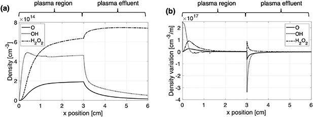
Figure 4. Example of plug flow model simulation results for the central bin (400 to 600 μm from the bottom of the plasma channel). In (a) the density evolution is plotted along the x-axis for different species, while (b) illustrates the corresponding spatial derivative.
Download figure:
Standard image High-resolution imageIn practice, for each bin and species implemented in the 2D model,  is found from the discrete derivative of the corresponding 0D plug flow model result for species
  . This approach enables the use of a 0D kinetics solver to solve the complex chemistry in the plasma channel, which greatly reduces the computation time, while retaining the spatial information needed for the resolution of the convection-diffusion equations. Of course, this approach comes at a cost: species diffusion perpendicular to the plug flow axis (crosswind diffusion) is completely uncoupled from the reaction kinetics. The error associated to this uncoupling will be further discussed in section 6.
The concentrations of species at the inlet are fixed at the experimental conditions: helium with 4500 ppm of  . Zero normal flux condition for each species is applied on all other boundaries:
 is the unit vector normal to the boundary and
  denotes the flux of species i.
5.2. Transport of species at the gas-liquid interface
The transport of reactive species at the gas-liquid interface is implemented through Henry's law, a partition condition that defines the ratio of concentrations at the interface:

where  and
and  are the concentrations in the liquid and gas phases and
  is the dimensionless Henry's constant. Additionally, flux continuity across the interface implies that:

where  and
and  are the species fluxes at the liquid and gas interface, respectively. The temperature-dependent, dimensionless Henry's constants for the species implemented in the 2D model are taken from [14].
5.3. Reaction-transport processes in the liquid phase
The transport of species in the liquid phase is computed by solving the species conservation equation considering reaction, diffusion and advection for 25 species and 52 chemical reactions:
where  is the concentration of species
  in the aqueous solution,
  is the diffusivity in water of species
  , as taken from [14],
  is the velocity vector field and
  represents the source and loss terms of species
  for all chemical reactions considered, in mol/(m3
 s). Initially, the liquid is considered as distilled water; all species' concentrations are set to zero except for
  and
and  which are set to a concentration of
  M. To investigate the chemistry in the liquid, we employed a chemical reaction set constructed specifically for chemical reactions between reactive oxygen and nitrogen species in aqueous solution, which was described previously in [14].
The liquid volume of the model represents a snapshot of the actual experimental situation. In reality, a dual-phase flow consisting of a steady moving train of liquid segments formed in the channel between gas bubbles is produced [1]. The formation of this dual-phase arrangement is highly dynamic, yet very reproducible. As the dynamic formation of the liquid segment-gas bubble train is complex to simulate, we limited our model to the time interval when the plasma stream contacts the liquid phase. A convective flow inside the liquid segments arises from the shear forces exerted by the microfluidic channel walls [38]. To include this movement in the model, the velocity of the top and bottom boundaries are set to the average liquid velocity of the water segment. In the results presented here, this velocity is 1.67 cm s−1 (Reynold number Re
 for a characteristic length of 1.5 mm, corresponding to the size of the microfluidic channel). This velocity refers to the average water segment velocity in the plasma-microfluidic experiment when a flow rate of 16.7 µl s−1 is used. The two other walls have a slip condition as they represent an air-water interface. Figure 5 illustrates the experimentally-observed liquid segment-gas bubble train formation (a) and how the movement inside the liquid volume was modelled (b).
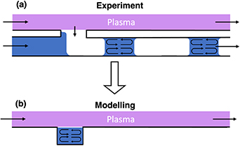
Figure 5. Schematic of the steadily moving liquid segment-gas bubble train observed experimentally (a). In the model, all the boundaries are stationary (b).
Download figure:
Standard image High-resolution imageThe 2D model we developed for the species production and transport in the plasma-microfluidic platform considers 20 species in the gas phase and 25 species in the liquid. Table 2 summarizes the species implemented in the 2D model. The 25 liquid species were taken directly from [14]. Among these species, only 18 can also exist in the gas phase; these are the 18 species that were included in the gas phase of the 2D model. The gas-liquid boudary is subject to Henry's law, as previously mentioned, and all other boundaries have a zero normal flux condition.
Table 2. Species implemented in the 2D model.
| Gas phase species |
|---|
| O2, N2, H2, O, N, H, OH, H2O2, HO2, O3, NO, N2O, NO2, NO3, HNO, HNO2, HNO3, NH |
| Liquid phase species |
|---|
| O2, N2, H2, O, N, H, OH, H2O2, HO2, O3, NO, N2O, NO2, NO3, HNO, HNO2, HNO3, NH, OH‒, O2 ‒, ONOOH, ONOO‒, H3O+, NO2 ‒, NO3 ‒ |
6. Results and discussion
The results of two distinct geometries will be presented. The first considers a liquid volume in contact with the plasma-forming zone, positioned between 24 and 26 mm from the main gas inlet (figure 1(a)). The second one uses a liquid volume in contact with the plasma effluent, and located between 33 and 35 mm from the main gas inlet (figure 1(b)). In both cases, the plasma power dissipation is taken as 1 W and the feed gas of 1.5 slm is humid helium (4500 ppm H2O) with oxygen (1 ppm) and nitrogen (4 ppm) impurities. Figure 6 shows the result of the first 2D simulation as presented in section 3, i.e. the gas velocity (a), temperature (b) and water vapour concentration (c), which are used as input to the plug flow models for each of the 11 bins used in this model. Figure 6(a) depicts the laminar flow pattern within the plasma channel, while figure 6(b) presents a temperature profile that increases along the channel length, and where the gas-water interface acts as a heat sink. Figure 6(c) displays the evolution of water vapour concentration in the plasma region. The water vapour concentration remains stable until the gas-water interface is reached, where evaporation triggers a significant increase in the water vapour concentration. Figure 7 illustrates the velocity field,  , inside the liquid (calculated as explained in section 5). Figure 7 demonstrates that the motion of the liquid segments within the microfluidic channels results in the formation of circulating flow patterns, enhancing the transport of reactive species within the droplets.
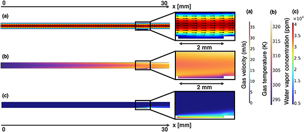
Figure 6. Gas velocity (a), gas temperature (b) and water vapour concentration profile (c) in the COST-jet channel solved as explained in section 3. (a) Depicts the laminar flow pattern in the channel, (b) shows the increasing temperature profile along the channel with the gas-water interface acting as a heat sink and (c) illustrates the evolution of water vapor concentration with the gas-water interface being a source of humidity.
Download figure:
Standard image High-resolution image
Figure 7. Velocity vector field inside the liquid volume solved as explained in section 5. The top and bottom boundaries are moving walls, which velocities are fixed as the water segments average velocity, and the two sides boundaries, that represent the gas-water interfaces, have slip conditions.
Download figure:
Standard image High-resolution imageFigure 8 depicts the evolution of  concentration for both plasma-liquid contact arrangements. The model predicts higher
  concentrations in the liquid when it contacts the plasma effluent compared to when it contacts the plasma-forming zone. After treatment, the average concentration of
  in the liquid is 34 µM for a water segments exposed to the plasma region, whereas a water segments in the plasma effluent region has an average
  concentration of 23 µM. This is explained by two reasons. First, the simulations show that the main destruction pathway of
  is through an electron impact reaction:

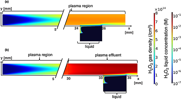
Figure 8. H2O2 concentration in plasma, plasma effluent and in the liquid for a plasma-liquid interaction zone located in the (a) plasma-forming zone and (b) plasma effluent solved as explained in section 5.
Download figure:
Standard image High-resolution imagewhich no longer takes place in the plasma effluent. Moreover, the main formation pathway of  is through the recombination of two
  radicals. Figure 9 shows the evolution of
  radicals both in the plasma-forming region and in the plasma effluent. Outside of the plasma-forming region, the
  radicals are quickly depleted to form
  while the previously mentioned electron impact reaction, which depletes
  no longer takes place.
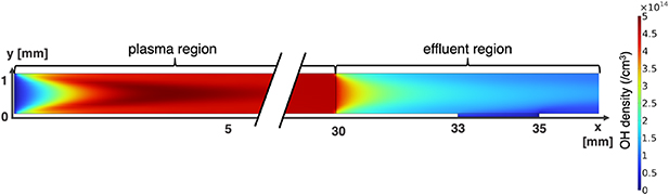
Figure 9. OH radical concentration in plasma and plasma effluent solved as explained in section 5.
Download figure:
Standard image High-resolution imageAs previously mentioned, the goal of this modelling work is to explain the experimental results reported recently [1] and to demonstrate the feasibility of a numerical representation of the plasma-microfluidic platform. In this experiment, the imposed liquid flow rate in the microfluidic channel was 16.7 µl s−1, corresponding to an average velocity of 1.67 cm s−1. With this velocity, the liquid segment-gas bubble combination travels through the 2 mm opening of the microfluidic device in 0.12 s, which can be transposed in the model as a liquid treatment time of 0.12 s. Hence, the experimental results were compared with a simulation of a liquid treatment time of 0.12 s. Of course, experimentally, the treated liquid is not analysed directly after treatment, and chemical reactions can occur in the liquid between treatment and analysis. However, further simulations showed that once the contact with the plasma or plasma effluent is removed, the average concentration variation of  is less than 1% for at least 90 s. Experimentally this is approximately the time between plasma treatment of the liquid and the moment when the treated liquid is analysed. The stability of the
  concentration after treatment was explained in previous work by Heirman et al [14]. The authors showed that most of the chemistry that leads to the production and loss of
  happens near the gas-liquid interface and that the reaction rates in the liquid bulk are at least 3 orders of magnitude smaller than at the interface. In the interface region,
  is mainly produced through
  and lost through
  . As the OH radicals originate from the plasma, these reactions no longer occur once the plasma or plasma effluent contact is removed. As in [14], we also observed in our simulations that
  is stable in the liquid without direct contact with gas-phase plasma-produced
  or
or  . Hence the concentration value of
  after 0.12 s treatment was taken for direct comparison with experimental values.
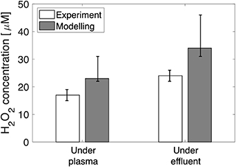
The  concentration in the treated liquid was measured experimentally with the titanium oxysulfate method presented in our own work [1] and in that of others [14, 39]. For a plasma power dissipation of 1 W and a microfluidic water flow rate of 16.7 µl s−1 (1 ml min−1 ), the concentration of
  in the treated liquid was experimentally measured for a liquid interaction zone under the plasma-forming region and under the plasma effluent region. Figure 10 shows the comparison of these experimental results with the average
  concentration in the liquid provided by the simulations after a treatment time of 0.12 s. The model predicts a higher concentration of
  than the experimental values, but with a reasonable margin; both experimental and modelling results differ by less than 50%, which is satisfactory considering the various approximations that were used.
Figure 10. Experimental and modelling comparison of H2O2 concentrations in the liquid volume, when the liquid is under the plasma and under the effluent. For explanation of the error bars of the modelling result, see text.
Download figure:
Standard image High-resolution image
One of the main simplifications used to model the plasma and effluent channel was to split the domain in bins and to solve an independent plug flow simulation for each of them. Through this approximation, the effect of transport of species between the different bins on the reaction kinetics is neglected. To investigate the impact of this approximation, further simulations were performed. We do not expect that the cross-talk between the bins would lead to a reaction kinetics that produces more  than the bin of maximal production, or less
  than the bin of minimal production. Thus, to estimate the minimum and maximum values of the average concentration of
  in the liquid, the species input (
 ) in the entire plasma and effluent channel was taken as the input in the bin of minimum and maximum
  production, respectively. In this way we can set an upper and lower limit on the expected
  production predicted by the model. These limits are illustrated as the error bars in figure 10. Note that both the maximum and minimum values do not change the conclusions drawn from the modelling results.
This extremum value investigation is quite straightforward for  in the liquid because it strongly correlates with the production of
  in the plasma and effluent channel. However, with the other species it may be necessary to look deeper into the production and destruction mechanisms to obtain minimum and maximum values. For example,
  is not formed in the gas phase, but only in the liquid through different reactions (such as
  or
or  ). Hence, an estimation of the maximum and minimum concentration values of this species requires a more thorough analysis.
The discrepancies between the experimental and modelling results can be explained by different limitations of the modelling approach. The most obvious one is the stationary boundary approximation. In the model all boundaries of the liquid are fixed in space, while in reality it is a dynamic system where the boundaries of the liquid segment are constantly moving. Also, the exact behaviour of the small gap between the plasma channel and the liquid is unknown. Its height, which is set to 100 μm based on experimental observation of the device, may exhibit certain variations due to the dynamic formation of the water droplet. This height is fixed experimentally by controlling the pressure inside the microfluidic device [1]. A verification is required whether there is plasma in the gap and if it makes direct contact with the liquid. However, based on the short recombination times of charged species outside of the COST-Jet's electrodes, as inferred from the 0D simulations, no chemical reactions are directly modelled in this gap. This applies to both studied cases, whether the liquid is under the plasma active region or under the plasma effluent region. Rather, the species are transported (by convection and diffusion) from the plasma channel to this region and are assumed not to react. Moreover, the species transport at the liquid interface through Henry's law will influence the chemical species concentration in the plasma-forming and plasma effluent regions, which in turn might influence the reaction kinetics. This is not taken into account in the model, i.e. There is no feedback loop to the 0D models from species transport at the liquid interface. The use of Henry's law constants is inherently limited to equilibrium conditions [14, 40, 41], which are not strictly met when significant transport takes place. However, no better implementation of the partition condition for reactive species between the gas and the liquid than Henry's law exists. Another limitation is related to the power density of the plasma discharge which is used to calculate the EEDF. It is taken as an average value for the whole plasma region. In reality it varies spatially within the plasma channel. These different limitations might explain the discrepancies between the modelling and experimental results. Nevertheless, the model provided key information on the main formation and transport pathways of reactive species from the plasma region to the liquid in the microfluidic device.
7. Conclusion
We presented a first modelling approach to simulate the COST reference plasma jet in contact with a microfluidic device. Taking advantage of the fast computation time of 0D modelling, we combined plug flow chemical kinetics models with 2D fluid dynamics-species transport models to obtain a quasi-2D model that provides spatially-resolved information on the formation and transport of reactive species produced by the COST-jet plasma discharge. This combined approach was based on the uncoupling of the plasma and plasma effluent reaction kinetics from the crosswind transport processes. The possible error associated with this assumption was discussed for the transport of hydrogen peroxide in the liquid. The modelling results were compared with experimental data. We found a good agreement with experimental observations for the concentration of hydrogen peroxide in the liquid. Key limitations of the modelling approach were discussed to guide the next steps needed to improve the model prediction abilities. The results mainly focused on hydrogen peroxide since experimental data were available. Nevertheless, the model we developed has the potential to give insight on the formation and transport of other plasma-generated reactive species. Moreover, the proposed modelling approach that combines a 0D plug flow model with 2D fluid dynamics simulation could be applied to simulate the complex chemistry of other plasma sources or any other system where the transport of chemical species occurs in a unidirectional gas flow at high Péclet number. The computational work presented here, combined with the plasma-microfluidic platform presented previously, set the basis both in terms of experimental work [1] and computational work for the use of standard and novel microfluidic devices in the context of plasma medicine.
Acknowledgments
The authors acknowledge the financial support from the Fond de recherche du Québec, the Natural Sciences and Engineering Research Council of Canada (including Grant Numbers RGPIN-06838 and RGPIN-06820), Gerald Hatch Faculty Fellowship from McGill University, the TransMedTech Institute through its main financial partner, the Apogee Canada First Research Excellence Fund, as well as from the Fund for Scientific Research Flanders (FWO; Grant Numbers G033020N and 1100421N).
Data availability statement
The data that support the findings of this study are openly available at the following URL/DOI: https://doi.org/10.5281/zenodo.10072906.