
Abstract
Non-equilibrium inductively coupled plasmas (ICPs) operating in hydrogen are of significant interest for applications including large-area materials processing. Increasing control of spatial gas heating, which drives the formation of neutral species density gradients and the rate of gas-temperature-dependent reactions, is critical. In this study, we use 2D fluid-kinetic simulations with the Hybrid Plasma Equipment Model to investigate the spatially resolved production of atomic hydrogen in a low-pressure planar ICP operating in pure hydrogen (10–20 Pa or 0.075–0.15 Torr, 300 W). The reaction set incorporates self-consistent calculation of the spatially resolved gas temperature and 14 vibrationally excited states. We find that the formation of neutral-gas density gradients, which result from spatially non-uniform electrical power deposition at constant pressure, can drive significant variations in the vibrational distribution function and density of atomic hydrogen when gas heating is spatially resolved. This highlights the significance of spatial gas heating on the production of reactive species in relatively high-power-density plasma processing sources.
Export citation and abstract BibTeX RIS

Original content from this work may be used under the terms of the Creative Commons Attribution 4.0 license. Any further distribution of this work must maintain attribution to the author(s) and the title of the work, journal citation and DOI.
1. Introduction
Non-equilibrium plasmas that contain hydrogen are of significant interest due to applications in surface processing [1–8], nanoelectronics [9–11], environmental science [12], aerospace [13–15] and the developing field of green chemistry [16–18].
Inductively coupled plasmas (ICPs) are often used in surface processing applications due to relatively high plasma density and flux of process-critical species to the substrate [19]. The production of atomic hydrogen is of particular interest due to its role in surface passivation [7], mild etching of 2D materials [20] and organic material processing [21, 22]. The relatively high plasma densities are driven by spatially localised power deposition from the inductive coil, which can lead to the formation of significant spatial gradients in the density and temperature of neutrals [23].
Previous work studying low pressure non-equilibrium plasmas includes the use of 0D plasma chemistry or global models [24–28]. 2D fluid models have been used to study spatially resolved hydrogen plasmas in applications related to negative ion sources used in magnetic confined fusion [29–34], negative ion sources for particle accelerators [35, 36], in the development of micro-discharges [37], and for surface processing [38]. 1D hybrid particle-in-cell models have also been developed to study the influence of atomic recombination on surfaces, the distribution of vibrational states within the plasma and velocity distributions of the negative ions [39–45]. Recently these 1D simulations have been used to study the advanced electrical plasma control strategies including voltage waveform tailoring plasmas [46], which demonstrated the importance vibrationally excited states [47].
At the relatively low power densities that correspond to capacitively coupled systems, detailed studies of vibrational kinetics have leveraged the reasonable assumption of an isothermal neutral gas temperature [46, 47]. Alternatively, fluid-based simulation approaches conducive to the modelling of 2D systems have considered spatially resolved gas heating with simplified reaction sets that do not focus upon the role of vibrationally excited states in low pressure hydrogen [29–34]. It is therefore of significant interest, as a means to develop an understanding of the high-power-density regimes with elevated gas temperatures relevant to industry, to account for both the vibrationally excited states and spatial gas-temperature gradients into a single model. This can be used to quantify the impact of setting the gas temperature to be isothermal on reactive species production and connected vibrational kinetics.
In this study, we use 2D fluid-kinetic simulations with the Hybrid Plasma Equipment Model (HPEM) [48] to investigate the spatially resolved production of atomic hydrogen, negative ions, and density of vibrationally excited states. The setup for the simulations is described in section 2 and the results are presented in section 3.
2. Simulation methods
2.1. Description of the model and simulation domain
A brief overview of the relevant details is given here. HPEM has a modular structure which allows for relevant physics of a system to be addressed using different techniques suitable for the physics of interest. In this work, we make use of the fluid kinetics Poisson module (FKPM), electron Monte Carlo simulation (eMCS), and the electromagnetics module (EMM). The FKPM solves the continuity, momentum and energy equations for all heavy particle species separately in combination with Poisson's equation for the electric potential and forms the basis of the simulation framework. Electron momentum is solved for using the drift-diffusion approximation. The EMM is used to solve the electric and magnetic fields that are a result of the current through the inductive coil. This is adjusted in order to give the specified power to the plasma, which in this study is fixed at 300 W. The eMCS simulates the interaction of electron pseudo-particles with the electric fields that are calculated using the FKPM and EMM. This is done using a Monte Carlo algorithm, which is described in detail in [49]. The algorithm in the eMCS calculates the electron energy distribution function (EEDF) for all domain points in the simulation. The resolution of the EEDF scales as the energy of the electrons increases. The resolution of the EEDF constructed in the eMCS module changes over the energy range from 0 to 1000 eV. There are a total of 500 energy bins for the eMCS module, where the lower energy levels between 0 and 5 eV have 100 bins. One hundred bins cover the range between 5 eV and 12 eV, then another 100 bins between 12 eV and 50 eV, 100 bins from 50 eV to 300 eV and 100 bins from 300 eV to 1000 eV. The eMCS module also calculates the corresponding electron impact rate coefficients and electron transport properties. These are used as inputs for the FKPM in the following iteration of the simulation. The use of the Monte Carlo method for the treatment of electrons helps to extend the validity of the fluid approach to the lower pressures considered in this study [50].
The simulation domain is based upon a modified Gaseous Electronics Conference (GEC) reference cell [51], as shown in figure 1.
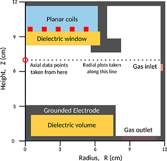
Figure 1. The simulation domain, showing the layout of the modified GEC reactor with five-turn planar coil. The locations where 'axial' data points for  cm, 7 cm), and radial profiles at Z = 7 cm are extracted at locations shown by the circle and dashed line, respectively.
Download figure:
Standard image High-resolution imageThe simulation domain has a radius of 12 cm, an axial height of 12 cm and a mesh resolution of 0.133 cm cell−1 in both the radial and axial directions. As shown in figure 1, a gap of 5 cm separates the grounded metal electrode from a quartz dielectric window, which has a thickness of 1.1 cm and separates the plasma region from a five turn coil. Hydrogen gas in its vibrational ground state is injected into the reactor volume, while a gas outlet at the base of the reactor utilises a fixed pressure in the plasma volume. The gas flow rate at the outlet is scaled with pressure to maintain a constant species residence time irrespective of pressure.
We set the power delivered to the ICP coil to be 300 W due to the availability of previous work in similar configurations [52, 53], and anticipate that the results can be extended to higher-power regimes [52, 53]. For this reactor, between 3.6 Pa and 25 Pa and 300 W, the plasma is expected to operate within the H-mode [53].
The simulations are run to reach a steady-state convergence as determined by considering the density of a selection of species and plasma parameters (density of atomic hydrogen, even numbers of the vibrational mode of hydrogen, plasma potential, and gas temperature) divided by the electron temperature. They are operated using two cores with the OPENMP architecture and typically require two days to reach convergence. They are run on a 64 core (32 physical) Intel Xeon E5-2683 v4 2.1 GHz with 128 GB total memory.
We also consider radial variations in plasma parameters for an axial location of Z = 7 cm, which is selected to correspond with the position of previously acquired experimental data [53].
2.2. Description of the reaction set
The diatomic nature of hydrogen molecules means that vibrational states play an important role in the distribution of energy in the system. The distribution of this energy occurs via several different interactions with other species in the plasma. A key process that excites vibrational states in the hydrogen molecule is electron impact excitation [54], both via eV and EV electron collisions. eV reactions are defined as being where electron collisions directly lead to vibrational excitation. As distinct from this, EV reactions are electron collisions that lead to electronic excitation before relaxation occurs into a vibrational state. After vibrationally excited states are formed, further electron impact reactions and collisions between vibrational states produce a vibrational energy distribution. This is important as the higher the vibrational state, the more energy is present in the vibrational mode. Through interactions with hydrogen atoms and molecules this energy can be translated back into kinetic energy through vibrational–translational (V–T) reactions, or the excited molecule may experience an electron impact dissociative attachment reaction to form a negative ion [54]. Therefore, an accurate treatment of the ways vibrational energy is distributed in the plasma is of significant interest when considering the gas temperature and formation of negative ions.
The reaction set is based upon that previously established by Diomede et al in [47]. It accounts for 16 neutral species, which include atomic hydrogen and the hydrogen molecule in their respective ground states and 14 vibrationally excited states of the hydrogen molecule. Five charged species are included, which are H+, H , H
, H , H− and electrons [39, 47, 55]. For this study we further develop the reaction set to include gas temperature dependent reactions for the vibrational–vibrational (V–V) and V–T reactions as well as reaction enthalpy, where V–V reactions correspond to the exchange of vibrational energy between vibrationally excited hydrogen molecules. This reaction set is shown in the
2.2.1. Heavy particle reaction rates.
The heavy particle reactions rates for each reaction are defined using the Arrhenius equation of the form:
where A is the Arrhenius parameter in units of cm3 s−1, n is a dimensionless scaling parameter, Eact. is the activation energy of the reaction in Kelvin, and  is the gas temperature in Kelvin.
Cross-sections for heavy particle ion–neutral reactions are incorporated using [55, 56]. Updates are made to include gas temperature dependent reaction rates for negative ion neutralisation with  and negative ion detachment with atomic hydrogen [54, 57, 58]. A Maxwellian distribution for the energy of the reacting species is assumed, and a reaction rate is calculated, as described in equations (2) and (3). The Arrhenius equation, identified in equation (1), is then fit to the calculated reaction rates between gas temperatures of 200 K and 3000 K using a least squares fitting routine. Two exceptions are for the ion–neutral conversion reactions for
  , where a fitting range of 200–9000 K is used. As the electric fields are expected to be relatively small in an ICP, it is assumed that ion temperatures are similar to the neutral gas temperature.
It is assumed that the energy distribution of each heavy particle reactant is described using a Maxwellian distribution:
where vR is the particle velocity, mR is the reduced collisional mass, k is the Boltzmann constant and  is the gas temperature [19]. This distribution is then used to calculate the gas temperature dependent reaction rate using equation:
where KAB is the reaction rate between particles A and B and  is the cross section in terms of particle velocity [19].
2.2.2. Vibrational state interactions.
We consider mono-quantum exchange of vibrational energy between hydrogen molecules via V–V and V–T interactions as well as multi-quantum exchange of energy via reactive and non-reactive atomic V–T processes.
The V–V reaction is defined as:

where v and w are the vibrational states of the interacting hydrogen molecules.
The reaction rates for the V–V reactions have been calculated using equation [58]:
where
As these reactions are directional for the case where v > w, detailed balance is carried out using equation (7) to find the reverse reaction rate:
where  is the reaction rate,
  is the ratio of the 1st and 2nd anharmonic constants of hydrogen (
 /
/ ) equal to 0.027 568 [59, 60], EI
is equivalent to hc
) equal to 0.027 568 [59, 60], EI
is equivalent to hc
 and
and  is the gas temperature. In a similar manner to the other heavy particle reactions, the calculated reaction rates for these reactions have then been fitted using an unweighted least squared fitting routine to equation (1) between gas temperatures of 300 K and 1200 K.
The V–T reactions are defined as:

for the forward reaction and

for the reverse reaction.
The reaction rates for these V–T reactions are calculated using the method described in [58]:
where
The equation is directional, such that the vibrational state of the products is lower than the reactants. This means that detailed balance is applied in order to calculate the reverse reaction rate as given by equation (12):
The exchange of energy between vibrational states can also occur through collisions with atomic hydrogen.

This reaction can occur through two reaction pathways, defined as reactive or non-reactive, and both have been added to the reaction set. The difference between the two cases is whether a hydrogen atom is exchanged in the collision, or not. Multi-quantum exchanges are also accounted for in the V–T reactions for atomic hydrogen, which are defined as when a transition between vibrational levels is higher than just through one level. Cross-sections for these multi-quantum V–T reactions are taken from [61] and unweighted least square fits of the reaction rates to equation (1) is carried out in all cases.
2.2.3. Electron impact reactions.
The cross sections of the electron impact reactions are added into HPEM such that the reaction rates are calculated from these and the EEDF derived from the eMCS within the code. The cross sections are extrapolated to cover the energy range from 0.0001 eV to 1000 eV and log–linear interpolation routines are used to calculate the reaction rates where exact cross-section data do not exist. Where a threshold exists for the electron impact reaction, the cross-section is set to zero for electron energies at and below this threshold. Superelastic collision cross sections are calculated through the principle of detailed balance for the eV vibrational excitation processes and included in the electron impact reaction set.
2.2.4. Surface interactions.
In this study we are most interested in the bulk-plasma properties and therefore implement a relatively simple treatment of the plasma–wall interaction. Previous work has demonstrated the importance of the thermal accommodation coefficient on the gas temperature [62]. The accommodation coefficient is kept constant across all of the surfaces. The results of previous simulations suggest that a value below 0.2 can have a large impact on the behaviour of molecular plasmas [62]. In this work, we therefore set the value of the thermal energy accommodation coefficient to be 0.4 for all surfaces [62]. The secondary electron emission coefficient, which we select to be  for all surfaces [37], is energy independent and depends only on the positive-ion flux to the surface.
The neutralisation and vibrational deactivation of species coming into contact with a surface is determined by two numbers. The sticking probability gives the probability that a species will undergo an interaction with a surface, and the return probability determines the return of species to the plasma. If a sticking probability of 1.0 is selected, all species interacting with the surface will 'stick' and with a return probability of 1.0, all of the 'stuck' species will return to the plasma. If a sticking probability of 0.1 is given, 10% of the species will interact with the surface and with a probability of 0.05, half of these interacting the species will return to the plasma as a new species. The values of the sticking and return probabilities for each species included in the model are shown in table 1. Vibrational deactivation from all 14 vibrationally excited states of hydrogen to the ground state occurs on all surfaces. All vibrational states deactivate to the ground vibrational state with a flux dependent sticking probability as described in [25].
Table 1. Sticking and return probabilities for each heavy-particle species included in the model.
| Wall interaction | Sticking probability | Return probability | Reference |
|---|---|---|---|
H H2 H2
| 0 | 0 | [40] |
H  H2 H2
| 0.1 | 0.05 | [40] |
H H H | 1.0 | 1.0 | [40] |
H H2 H2
| 1.0 | 1.0 | [40] |
H H2 H2
| 1.0 | 1.0 | [40] |
H H H | 1.0 | 1.0 | [40] |
H H H | 1.0 | 1.0 | [40] |
H2(v = 1)  H2(v = 0) H2(v = 0) | 0.1 | 0.1 | [25] |
H2(v = 2)  H2(v = 0) H2(v = 0) | 0.2 | 0.2 | [25] |
H2(v = 3)  H2(v = 0) H2(v = 0) | 0.3 | 0.3 | [25] |
H2(v = 4–9)  H2(v = 0) H2(v = 0) | 0.4 | 0.4 | [25] |
H2(v = 10–13)  H2(v = 0) H2(v = 0) | 0.5 | 0.5 | [25] |
H2(v = 14)  H2(v = 0) H2(v = 0) | 1.0 | 1.0 | [25] |
The temperature of all surfaces is fixed at 325 K.
The gas temperature is calculated from the weighted average temperature of each species, defined as:
where Tg
is the average gas temperature, Ti
is the gas temperature of neutral species i, and ni
is the corresponding density. For simulations where the temperature of the neutral gas is determined self-consistently, i.e. not set to be isothermal, the enthalpy change of all heavy-particle species is calculated. In cases where the gas temperature is calculated, heating via the Frank–Condon principle [63] has been accounted for and the energy exchange between the electrons and the heavy species has been set to zero where relaxation through photon emission can be expected. The ΔH for the exchange of kinetic energy in the heavy particle reactions has been listed for each reaction in the
2.2.5. Temperature of atomic hydrogen.
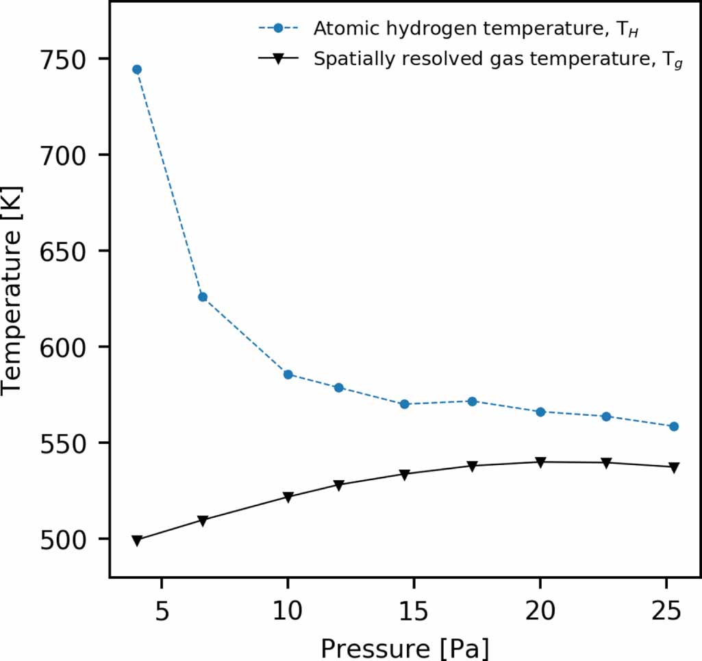
In low-pressure hydrogen plasmas, atomic hydrogen that is produced via electron-impact dissociation of molecular hydrogen through the repulsive  state receives a significant quantity of kinetic energy [64]. It is not possible to fully account for this effect when operating under the assumption that neutrals are isothermal, particularly in the relatively low-pressures 4–25 Pa considered here. Figure 2 shows the temperature of atomic hydrogen and the gas temperature, which is determined self-consistently via equation (14), with respect to the pressure of the neutral gas.

Figure 2. Atomic hydrogen temperature, TH, and spatially resolved gas temperature as determined equation (14) at  cm, 7 cm). Applied power 300 W.
Download figure:
Standard image High-resolution imageAt a pressure of 4 Pa, the atomic hydrogen temperature is observed to be 250 K higher than the average gas temperature. As the pressure increases, the difference between the atomic hydrogen temperature and the gas temperature decreases. At pressures above 15 Pa the difference in the atomic hydrogen temperature and the average gas temperature is approximately 30 K. As such, the isothermal approximation is likely to be less accurate for the relatively low-pressure cases 4–15 Pa. This trend is qualitatively similar to that previously observed in [24].
3. Results
3.1. Macroscopic plasma properties
An overview of the macroscopic plasma parameters at 20 Pa is shown in figure 3.
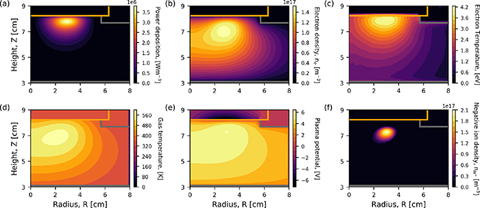
Figure 3. Spatial variation of the (a) power density, (b) electron density, (c) electron temperature, (d) gas temperature, (e) plasma potential, and (f) negative ion density. Applied power 300 W, gas pressure 20 Pa.
Download figure:
Standard image High-resolution imageThe power density is observed in figure 3(a) to be at a maximum below the dielectric window, and is positioned below the third coil away from the axis of symmetry with a value of  W m−3.
The electron density, shown in figure 3 peaks beneath the planar inductive coil, as has previously been widely observed experimental works [19, 23]. This corresponds to the location close to where the power density is highest, as shown in figure 3(a). The highest observed density in figure 3(b) is  m−3.
m−3.
The electron temperature, shown in figure 3(c), reaches a maximum nearby to the dielectric window of 4 eV.
The gas temperature is observed in figure 3(d) to be highest beneath the planar coil, and reaches a maximum of 573 K. For increasing radial position from the central axis its temperature decreases towards that of the wall at 325 K. This is consistent with expectation and highlights the presence of temperature gradients.
The plasma potential is observed in figure 3(e) to be at a maximum at a radial distance of R = 3 cm and reaches a value of 5.5 V, which is consistent with that measured in previous experiments in similar systems [53]. A negative potential is also observed within the dielectric material (Z = 8 cm), which is an artefact of its method of calculation from the electric field determined at each mesh point. This can lead to a negative plasma potential being observed within materials.
The inclusion of vibrational states into the gas chemistry allows the simulation to calculate the negative ion density self-consistently. The negative ion density is observed in figure 3(f) to be at a maximum in the bulk of the plasma of  m−3. This is higher than the observed electron density, which suggests that the plasma in this region is electronegative. The negative ion density decreases by several orders of magnitude away from this localised maxima in all directions. This location of maximum negative ion density aligns with the maxima of the plasma potential, as shown in figure 3(e). The negative ion maxima is surrounded by a halo of H3
+ ions as a result of recombination in this region lowering the H3
+ density. The density of H+ is seen to be at a maximum where the H− is at a maximum. The sum of the positive species and negative species in this region results in a quasi-neutral plasma. The production of negative ions is observed to be lower in the location of highest plasma potential, and destruction is also highest in this region. This suggests that the negative ions are produced in the bulk of the plasma and diffuse towards the location of highest plasma potential.
m−3. This is higher than the observed electron density, which suggests that the plasma in this region is electronegative. The negative ion density decreases by several orders of magnitude away from this localised maxima in all directions. This location of maximum negative ion density aligns with the maxima of the plasma potential, as shown in figure 3(e). The negative ion maxima is surrounded by a halo of H3
+ ions as a result of recombination in this region lowering the H3
+ density. The density of H+ is seen to be at a maximum where the H− is at a maximum. The sum of the positive species and negative species in this region results in a quasi-neutral plasma. The production of negative ions is observed to be lower in the location of highest plasma potential, and destruction is also highest in this region. This suggests that the negative ions are produced in the bulk of the plasma and diffuse towards the location of highest plasma potential.
3.2. Variation in the electron density and temperature with gas pressure
The variation of the electron density and temperature with respect to gas pressure between 4 and 25 Pa is shown in figure 4.
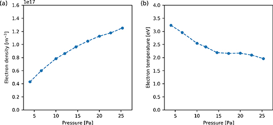
Figure 4. (a) Electron density and (b) electron temperature with respect to gas pressure as determined at ( cm, 7 cm). Applied power 300 W.
Download figure:
Standard image High-resolution imageIn figure 4(a), as the pressure in the reactor is increased, the electron density is observed to increase between 4 Pa and 25.3 Pa, from  to
to  respectively. The rate of increase in the electron density decreases as the pressure increases.
In figure 4(b), the electron temperature is observed to decrease from 3.2 eV to 2.0 eV as the pressure is increased from 4 Pa to 25.3 Pa. The electron temperature is observed to trend towards an electron temperature of approximately 2 eV. The observed trends are comparable to previous observations in similar reactor systems [24, 53].
3.3. Atomic hydrogen densities
As described in section 1, the 2D simulations enable comparison of spatial variation in the plasma response to pressure for two distinct cases: (1) where the temperature of the neutral gas is isothermal, and (2) where its temperature is self-consistently determined. In this study we have chosen five isothermal cases, 325 K, 450 K, 600 K, 750 K and using an isothermal temperature equivalent to the maximum gas temperature Tg, max observed in the self-consistent and spatially resolved case. Our motivation for this selection is:
- 325 K is the wall temperature of the reactor, and in the isothermal case it is assumed that all temperature gradients are zero.
- 450 K corresponds to the operating conditions of previous experiments [53, 65, 66].
- 600 K corresponds to the configuration of previously undertaken simulations with an isothermal neutral gas [26].
- 750 K is an over-approximation of the gas temperature to observe the enable observation of the corresponding impact.
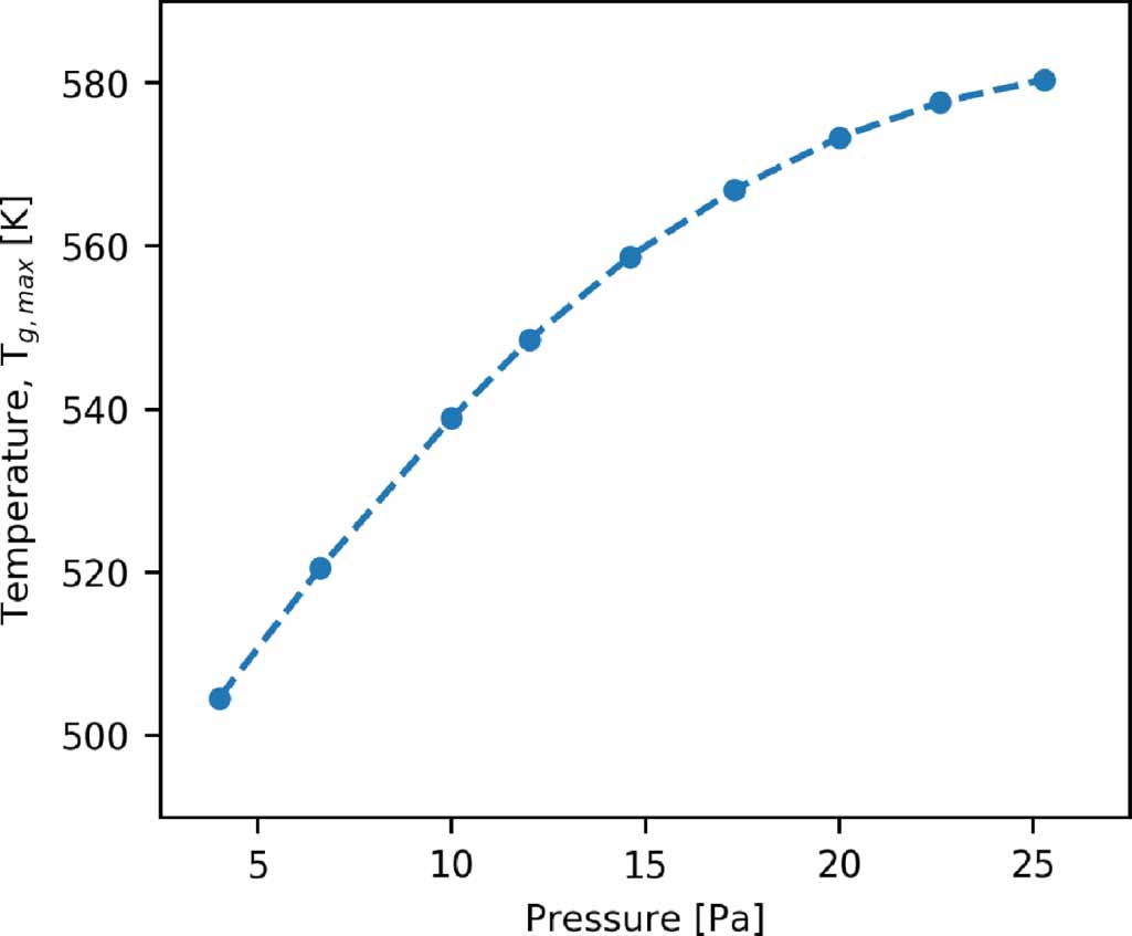
- The maximum temperature Tg, max is determined for each pressure case. The motivation for this is that we can consider these simulations as being similar to the spatially resolved gas temperature, but without the temperature gradients. This will therefore highlight the role of temperature gradients on the plasma response. The variation in the maximum neutral gas temperature with respect to pressure is shown in figure 5.

Figure 5. Variation in the maximum value of the gas temperature, as determined self-consistently, with respect to the pressure of the neutral gas. Applied power 300 W.
Download figure:
Standard image High-resolution imageFigure 6 shows the atomic hydrogen density as determined using an isothermal neutral gas, and when its temperature is spatially resolved for two pressure cases 6.6 Pa and 20 Pa.
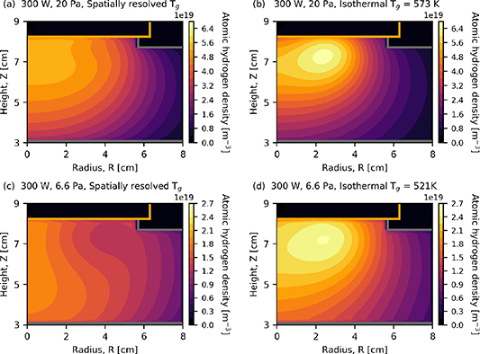
Figure 6. Density of atomic hydrogen at 20 Pa as determined using (a) spatially resolved and (b) isothermal neutral-gas temperatures. Panels (c) and (d) show the results corresponding to 6.6 Pa. For the isothermal cases (b) and (d), the gas temperature, which corresponds to  as determined in the spatially resolved cases, is noted in the panel. Applied power 300 W.
Download figure:
Standard image High-resolution imageAt 20 Pa, figures 6(a) and (b), the maximum density of the atomic hydrogen is observed to be  m−3 for the isothermal case and
  m−3 when the gas temperature is spatially resolved. The location of the maximum hydrogen density is observed to be closer to the radial centre of the reactor for the spatially resolved case. The temperature of the gas in this region at 20 Pa is observed in figure 3(d) to be above 500 K and varying by ±75 K. This 75 K difference appears to be responsible for the observed difference in the atomic hydrogen density in the 20 Pa isothermal case, figure 6(b) and highlights the importance of spatially resolving the gas temperature.
At 6.6 Pa, figure 6(c), the atomic hydrogen density determined using a spatially resolved gas temperature exhibits a spatial shift in the location of the maximum towards the bottom electrode and central axis when compared to the isothermal case, shown in figure 6(d). At 6.6 Pa the maximum gas temperature, as shown in figure 5, is 521 K. The maximum density of atomic hydrogen is also 30% lower for the spatially resolved case, where the spatially resolved and isothermal values are  m−3 and
  m−3 respectively.
As discussed at the start of section 3.3, the use of an isothermal gas temperature may be a reasonable approximation if one were to take the maximum temperature observed in the reactor. It may also be reasonable to approximate the gas temperature from measurements taken close to the grounded electrode [53]. However, using approximations of the gas temperature is likely to produce a poor estimate of species densities close to where the power is being deposited. This is evidently the case when considering atomic hydrogen densities as shown in figure 6.
To further investigate the differences between the cases where the gas temperature is treated as isothermal, or as distinct from this spatially resolved, the density of atomic hydrogen is shown in 7 with respect to pressure and radial location.
It is observed in figure 7(a) that the atomic hydrogen density reaches a maximum near to the central axis of the reactor R = 0, varying from  m−3 to
  m−3 over the pressure range of 4 Pa to 25.3 Pa. The atomic hydrogen density is also observed to increase as the pressure increases. This is consistent with previous experimental observations in similar conditions [52].
In figure 7(b) a similar trend to figure 7(a) is observed. Consistent with the results shown previously in figure 6, the density of atomic hydrogen is significantly larger, independent of radial location and gas pressure, when the gas temperature is treated as isothermal relative to the self-consistently determined case shown in figure 7(a).
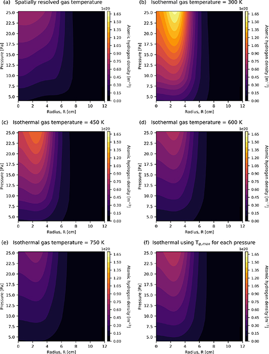
Figure 7. Radial variation in the density of atomic hydrogen at an axial location Z = 7 cm (see figure 1) as determined using (a) spatially resolved gas temperature, and isothermal gas temperatures for (b) 325 K, (c) 450 K, (d) 600 K, (e) 750 K and (f) maximum gas temperature  determined at each pressure. Applied power 300 W.
Download figure:
Standard image High-resolution imageIn figure 7(c), increasing the isothermal gas temperature to 450 K, the overall distribution of the atomic hydrogen is observed to be qualitatively similar to the calculated case in figure 7(a). However, the maximum density of the atomic hydrogen is observed to be higher by 40%, increasing from a maximum of  m−3 to
  m−3.
m−3.
Increasing the isothermal gas temperature to 600 K, the resulting atomic hydrogen density is shown in figure 7(d) and is observed to be similar to the calculated gas temperature case in figure 7(a), although the location of maximum atomic hydrogen density is observed to be slightly more localised at a larger radial extent in the 600 K case.
At an isothermal temperature of 750 K, shown in figure 7(e), the atomic hydrogen density is observed to be approximately 20% lower, where the maximum density is  m−3 at 750 K, compared to
  m−3 for the spatially resolved case. The distribution of the atomic hydrogen is also observed to be more closely confined to the radial centre at low pressures compared to the spatially resolved gas temperature case, shown in figure 7(a).
Figure 7(f) shows the density of atomic hydrogen for the case of an isothermal gas temperature, where its value is the maximum gas temperature  determined using the spatially resolved case. The resulting density distribution is observed to be broadly similar to that for figure 7(a), where the gas temperature is self consistently determined. It is important to note that the location of the maximum density is observed to occur at a slightly larger radial extent in the former case.
Overall, the results of figure 7 show that the choice of isothermal gas temperature is important when considering the atomic hydrogen density, e.g. comparing figures 6(a) and 7(b). The difference that is observed is also seen to become more significant as the neutral-gas pressure increases.
3.4. Vibrationally excited states of H2
The spatial variation of the vibrational density function is shown in figure 8 for a fixed axial height of Z = 7 cm.

Figure 8. Radial variation in the vibrational distribution function at Z = 7 cm at a neutral pressure of 10 Pa for (a) isothermal gas temperature:  K and (b) spatially resolved gas temperature. Panels (c) and (d) show the distribution functions for an increased pressure of 20 Pa, where the neutral gas temperature in the isothermal case
  K. The isothermal gas temperatures correspond to the maximum value observed in the spatially resolved cases. Applied power 300 W.
Download figure:
Standard image High-resolution imageSpatially resolved vibrational density functions for 10 Pa and 20 Pa are shown in figure 8 for cases where the gas temperature is isothermal (figures 8(a) and (c)) and spatially resolved (figures 8(b) and (d)), respectively. In both cases, a plateau in the distribution function is observed for vibrational levels 4–8, and this is consistent with the results of previous work [39]. Distinct behaviour is observed for the two cases for relatively high vibrational levels, i.e. larger than v = 10, and for relatively large radial extents R = 6–8 cm. In this region, for 10 Pa the densities of the higher-level vibrational states become depleted when gas heating is spatially resolved (figure 8(b)) relative to the isothermal case (figure 8(a)). This depletion of the higher vibrational states is more pronounced at higher pressures, as observed in figures 8(b) and (d).
The neutral gas density plays an important role in the production of vibrational states through the electron–neutral collisions. To investigate the changes in the neutral density, figure 9 shows the spatial variation in the density of ground-state molecular hydrogen at 20 Pa.
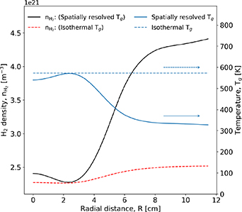
Figure 9. Spatial variation in the density of ground-state molecular hydrogen, evaluated at an axial position Z = 7 cm, for cases where the gas temperature is spatially resolved and isothermal. The corresponding temperature of the neutral gas is also shown. Pressure 20 Pa. Applied power 300 W.
Download figure:
Standard image High-resolution imageFigure 9 shows that the density of ground-state molecular hydrogen decreases towards the central axis for both spatially resolved and isothermal gas-temperature cases. In the isothermal case, where the gas temperature is set to be the maximum value determined in a self-consistent simulation, minimum density is almost the same as that when spatial resolution is employed. This is consistent with what can be expected from the ideal gas law. The difference in the neutral gas density at relatively large radial extents is much more pronounced in the spatially resolved temperature case, at R = 12 cm  m−3 compared to
  m−3. This mirrors what is observed in the gas temperature. In the isothermal case, decreases in the density can only be attributed to reactions that excite or dissociate the ground state hydrogen. This trend is expected to be observed at other pressures.
The observation of vibrational state depletion at relatively large radial extents is consistent with a relative increase in the neutral-gas density shown in figure 9, and electron–neutral collision frequency for the spatially resolved gas temperature case, where the temperature of the neutral gas is allowed to decrease for increasing values of R. Similar behaviour is observed at 20 Pa, shown in figures 8(c) and (d) for isothermal and spatially resolved gas temperatures, respectively.
Figure 10 shows vibrational distribution functions (VDFs) with respect to axial location, where the data is extracted at R = 2.4 cm to correspond to the location of maximum power deposition, shown previously in figure 3(a).
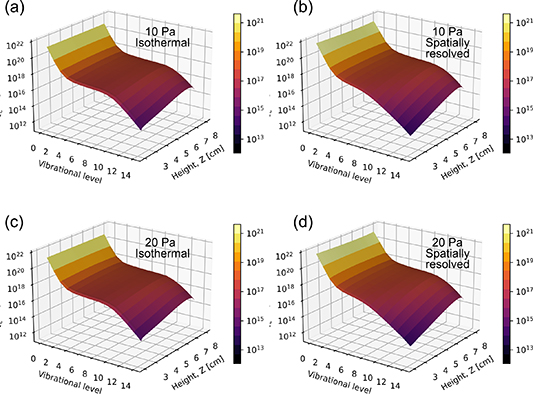
Figure 10. Vibrational distribution functions for (a) 10 Pa, Tg = 539 K and (b) 10 Pa with a spatially resolved temperature (c) 20 Pa, Tg = 573 K (d) 20 Pa with a spatially resolved temperature at an radial extent of 2.4 cm. Applied power 300 W.
Download figure:
Standard image High-resolution imageIt is observed in figure 10 for all cases that a plateau region exists between v = 4 and v = 10. This is consistent with expectations and what has previously been observed in figure 8. Using an isothermal gas temperature, there is a decrease in the vibrational-state density above v = 10 observed with a decreasing axial height Z, i.e. moving towards the bottom electrode in figure 1. This decrease is not as clearly visible for vibrational states lower than v = 10. Comparing figures 10(a) and (c), the decrease in the densities is more pronounced at 20 Pa (figure 10(c)) than at 10 Pa (figure 10(a)). This can reasonably be expected due to the increased rate of collisional de-excitation in the higher-pressure case. A similar trend is observed when implementing a spatially resolved gas temperature in figures 10(b) and (d).
Comparing the isothermal and spatially resolved gas-temperature cases, shown in figures 10(a) and (b) for 10 Pa respectively, the densities are observed to be similar for decreasing axial height with the most significant difference observed at higher vibrational levels (v  10). This can reasonably be attributed to a higher average electron temperature and density in this region relatively close to the central axis, which increases the electron-impact excitation rate.
In figures 10(c) and (d), which correspond to the higher pressure case of 20 Pa, trends are observed to be similar to the observations at 10 Pa. The vibrational state densities decrease with decreasing axial height, where a relatively large drop is observed when the gas temperature is spatially resolved.
In figure 11 the vibrational density distributions at increasing radial extents are shown for 10 Pa and 20 Pa. The isothermal gas temperature is set at the maximum temperature observed when implementing a spatially resolved gas temperature, as shown in figure 7(f).

Figure 11. Vibrational distribution functions for (a) 10 Pa, Tg = 539 K and (b) 20 Pa, Tg = 573 K at radial locations 0 cm, 4 cm and 8 cm. Applied power 300 W.
Download figure:
Standard image High-resolution imageThe VDF is observed to be consistent with previous work, where there is a superthermal plateau region observed in the vibrational state densities between v = 4 and v = 8 [39]. This distribution is associated with the EV vibrational excitation caused by electron impact reactions [67], and is further accentuated by the H atom V–T reactions, which depress the tail of the vibrational energy distribution. The plateau of the VDF, as well as the higher vibrational states above v = 9, is observed to be higher at R = 4 cm compared to both R = 0 cm and R = 8 cm. This location is associated with a maximum in the electron temperature, which increases the production of vibrational states through electron impact excitation. The VDF at R = 0 cm has a higher density of excited states between v = 1 and v = 11 compared to R = 8 cm, while above v = 12 the density of vibrational states is higher than at R = 0 cm.
In figure 12 the vibrational density distributions at increasing radial extents are shown for 10 Pa using a self consistently calculated gas temperature. The gas temperature in the reactor is also shown.
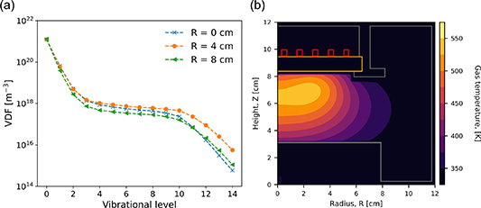
Figure 12. (a) Vibrational distribution functions at radial locations 0 cm, 4 cm and 8 cm for a spatially resolved gas temperature at 10 Pa. (b) The calculated gas temperature within the reactor. Applied power 300 W.
Download figure:
Standard image High-resolution imageIn figure 12(a), the VDF is observed to be consistent with what is observed in the isothermal case, figure 11(a), where there is a superthermal plateau region observed in the vibrational state densities between v = 4 and v = 8 [39].
The observed vibrational densities at R = 4 cm is also observed to be lower in the spatially resolved case, compared to the isothermal case shown in figure 11. For the R = 0 cm case, the higher vibrational states between v = 1 and v = 3 are similar to the R = 4 cm while the R = 8 cm case is lower. In this spatially resolved gas temperature case, this can be attributed to lower reactivity of the V–V and V–T reactions where the combination of the lower gas temperature, and lower electron temperature combine to reduce the excitation of higher vibrational states at large radii, whilst diffusion to the larger radii results in a slightly increased density compared to the reactor centre.
In figure 13 the vibrational density distributions at increasing radial extents are shown for 20 Pa using a self consistently calculated gas temperature. The gas temperature in the reactor is also shown.

Figure 13. (a) Vibrational distribution functions at radial locations 0 cm, 4 cm and 8 cm for a spatially resolved gas temperature at 20 Pa. (b) The calculated gas temperature within the reactor. Applied power 300 W.
Download figure:
Standard image High-resolution imageAt a higher pressure of 20 Pa, shown in figure 13, the vibrational distribution is observed to have a comparable distribution as at the lower pressure of 10 Pa with a similar superthermal plateau.
At the higher pressure shown in figure 13, the density of the plateau region is observed to be somewhat similar to the 10 Pa case shown in figure 12. It is observed that away from the maximum electron temperature at 4 cm, the vibrational density distribution has a more pronounced decrease in the excited states, when compared to the 10 Pa case. This is attributed to a higher reaction rate of the V–V an V–T reactions due to the higher pressure.
This is consistent with observations in the isothermal case and in previous work [68].
It is important to note that figures 8–13 emphasise the influence that the gas temperature gradient has on the distribution of the vibrational energy in the system. Choosing an arbitrary gas temperature for an isothermal condition does not allow for the V–V and V–T states to evolve across the reactor away from where the power is deposited. It can be expected that, if the power density of the reactor was increased, resulting in larger temperature gradients, the difference between the observed VDFs would be even more pronounced when comparing isothermal and spatially resolved gas-temperature cases.
3.5. Influence of gas temperature on the distribution of atomic hydrogen and negative ions
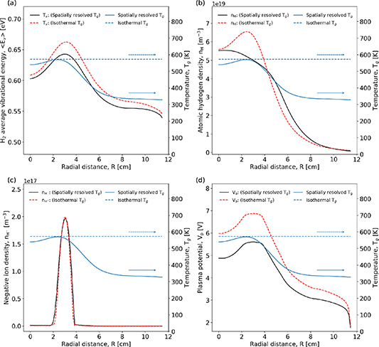
Figure 14 shows the spatially resolved H2 average vibrational energy, atomic hydrogen density, negative ion density and plasma potential, for cases where the gas temperature is spatially resolved and isothermal.
Figure 14. Radial profiles of (a) average vibrational energy of molecular hydrogen, (b) atomic hydrogen density, (c) negative ion density, (d) plasma potential at Z = 7 cm. Profiles of the corresponding spatially resolved and isothermal gas temperature are shown in each panel for reference. Pressure 20 Pa and applied power 300 W.
Download figure:
Standard image High-resolution image
Figure 14 shows that the gas temperature for the spatially resolved case has a peaked profile reaching a maximum of 573 K. This value is therefore applied to the isothermal case. In figure 14(a) the average energy of the vibrational states is shown, which has been calculated using a weighted average energy of the vibrational states:
where Ev is the energy of each vibrational level in eV and nv is the density of each vibrational state from v = 1 to v = 14. The vibrational energy is observed to be lower, across the full radial extent, for the spatially resolved case. This suggests that the energy stored in the vibrational states is higher when using an isothermal gas temperature. The average vibrational energy decreases for increasing radial extents, approaching 0.516 eV for both gas-temperature calculation methods at the radial boundary. This is consistent with expectation because in this region few electron impact excitation reactions occur, which means that less energy can be coupled into vibrational states. The isothermal gas temperature case has a smoother radial profile, which is to be expected due to a spatially uniform gas temperature that underpins similar V–T and V–V reaction rates. The peak in average vibrational energy is observed to be at R = 3.7 cm, which is where the power density is maximised as shown previously in figure 3(a). This is the location where the mean electron energy can reasonably be expected to be at a maximum, resulting in maximal vibrational excitation. It is observed that the isothermal case has larger values of average H2 vibrational energy in this location compared to the spatially resolved case. This difference can reasonably be explained by distinct profile of the plasma potential, described below and shown in figure 14(d), which results in a relatively low electron temperature in the spatially resolved case.
In figure 14(b) the atomic hydrogen density is observed to be higher in the isothermal case, and located where the power density is highest, see figure 3(a). This is consistent with expectations as a key process for the production of atomic hydrogen is electron impact dissociation. In the spatially resolved gas temperature case, the effects of diffusion are accounted for in the determination of the radial H-atom density profile.
In figure 14(c) the negative ion density is shown. The density of negative ions appears to be virtually the same for the spatially resolved and isothermal gas-temperature cases. A small difference in the width of the distribution is observed at R = 2 cm. This similarity suggests that the gas temperature plays only a minor role in the negative ion density distribution. This is consistent with expectations as the electric field plays a large role in the transport of negative ions in the plasma. The gas temperature dependent diffusion of this species is small compared to the diffusion due to electric fields, resulting in the maximum negative ion density being located where the plasma potential is at a maximum, as shown in figure 14(d).
The plasma potential is shown in figure 14(d) and reaches a maximum where the power density is maximal for both gas temperature cases, which is consistent with expectations. It is observed that the plasma potential is higher by 1 V when a isothermal gas temperature is employed. This result can be attributed to the additional transport of neutral species away from where the power is being deposited as a result of the introduction of a gas-temperature gradient. A correspondingly lower electron density in this region can reduce the ionization rate and thereby the plasma potential.
4. Conclusion
In this study, we use fluid-kinetic simulations with the HPEM to investigate the spatially resolved production of atomic hydrogen and underpinning distribution of vibrationally excited states in a low-pressure inductively coupled hydrogen plasma (ICPs, 10–20 Pa or 0.075–0.15 Torr, 300 W). The reaction set is developed from previously established work to incorporate gas-temperature dependent reaction rates for heavy particles and reaction enthalpies, where we track the kinetics for 14 vibrationally excited states. The results show that spatially resolving the gas temperature, as distinct from treating it to be isothermal, can significantly impact VDF and connected density of atomic hydrogen due to the formation of spatial gradients in the neutral density at fixed pressure. In particular, higher level vibrational states v > 10 become depleted at relatively large radial extents R > 6 cm from the central axis at 10–20 Pa, and this effect becomes more pronounced for higher pressures. In contrast, the spatial distribution of the negative ion density is relatively insensitive to gas-temperature gradients and is more closely correlated with the plasma potential. This highlights the role of spatial gas heating on the production of reactive species in relatively high-power-density plasma processing sources.
Acknowledgment
We wish to thank Pascal Chabert and Erik Wagenaars for useful discussions. This work was funded by the Engineering and Physical Sciences Research Council, Grant Reference Number EP/L01663X/1. Vasco Guerra was supported by the Portuguese FCT-Fundação para a Ciência e a Tecnologia, under funding to IPFN Lab (DOI: 10.54499/LA/P/0061/2020) and projects (DOI: 10.54499/UIDB/50010/2020, 10.54499/UIDP/50010/2020). The participation of M. J. Kushner was supported by the US National Science Foundation (PHY-2009219) and the US Department of Energy's Office of Fusion Energy Science (DE-SC0020232).
Data availability statement
The data that support the findings of this study are openly available at the following URL/DOI: https://doi.org/10.15124/cf0c6a12-79e2-4b6d-af78-a4a1fa6900ea.
Appendix:
This appendix contains the H2 reactions included in the model.
Table 2. Heavy particle reactions with associated parameter values for the Arrhenius equation applied within HPEM. Reaction rate coefficient is cm3 s−1 for two-body reactions.
| No. | Reaction | A (cm3 s−1) | n |
 (K) (K) | ΔH (eV) (eV) | Reference |
|---|---|---|---|---|---|---|
| 1 | H + H + H H2 + H H2 + H
|

| −0.01 | 0 | 0 | [69] |
| 2 | H + H + H H+ + H2 + H2 H+ + H2 + H2
|

| 0.65 | 39 257 | −4.44 | [70] |
| 3 | H + H + H H H + H + H + H + H + H + H |

| 0.33 | 72 782 | −10.8 | [70] |
| 4 | H2 + H H+ + H2 H+ + H2
|

| 0.04 | 0 | 0 | [70] |
| 5 | H+ + H  H+ + H H+ + H |

| 0.39 | 0 | 0 | [40, 71] |
| 6 | H + H + H H H + H + H |

| 0 | 0 | 1.76 | [70] |
| 7 | H + H + H H H + H2 + H2
|

| 1.39 | 0 | 0 | [70] |
| 8 | H− + H H− + H2 H− + H2
|

| 0.09 | 0 | 0 | [70] |
| 9 | H− + H H2 + H + e H2 + H + e |

| 1.27 | 15 638 | 0 | [70] |
| 10 | H− + H  H− + H H− + H |

| 0.33 | 0 | 0 | [40, 71] |
| 11 | H− + H  H2 + e H2 + e |

| −0.022 | 403 | 0 | [54] |
| 12 | H− + H H2 + H2 H2 + H2
|

| −0.5 | 0 | 12.91 | [57, 58] |
| 13 | H− + H H2 + H2 H2 + H2
|

| −0.5 | 0 | 12.83 | [56] |
| 14 | H− + H+
 H2 + H2 H2 + H2
|

| −0.5 | 0 | 10.15 | [56] |
| 15 | e + H H + H H + H |

| −0.4 | 0 | 10.97 | [56] |
| 16 | e + H H + H + H H + H + H |

| −0.8 | 0 | 4.69 | [56] |
| 17 | e + H H2 + H H2 + H |

| −0.8 | 0 | 9.21 | [56] |
Table 3. Non-vibrational electron impact reactions. Reaction rates calculated in the eMCS module within HPEM from cross sections in associated references.
| No. | Reaction | Δ H (eV) | Reference |
|---|---|---|---|
| 18 | e + H H2 + e H2 + e | 0.0 | [72, 73] |
| 19 | e + H2(v)  H2(v) + e H2(v) + e | 0.0 | [72, 73] |
| 20 | e + H  H + e H + e | 0.0 | [74, 75] |
| 21 | e + H H+ + H + 2e H+ + H + 2e | 0.0 | [54] |
| 22 | e + H  H+ + 2e H+ + 2e | 0.0 | [76] |
| 23 | e + H H H + 2e + 2e | 0.0 | [77] |
| 24 | e + H H + H H + H + e
a + e
a
| 0.0 | [78] |
| 25 | e + H H + H H + H + e
b + e
b
| 0.0 | [78] |
| 26 | e + H H + H + e (via H + H + e (via  ) ) | 4.38 c | [78] |
| 27 | e + H H + H + e (via H + H + e (via  ) ) | 0.0 | [78] |
| 28 | e + H H + H + e (via H + H + e (via  ) ) | 0.0 | [78] |
| 29 | e + H H + H + e (via H + H + e (via  ) ) | 0.0 | [78] |
a
H –3) density not resolved
b
H(n = 2–3) density not resolved
c
This contribution to the energy is a result of the difference in the energy threshold of the electron impact cross section and the enthalpy of formation for the two H atoms.
–3) density not resolved
b
H(n = 2–3) density not resolved
c
This contribution to the energy is a result of the difference in the energy threshold of the electron impact cross section and the enthalpy of formation for the two H atoms.
Table 4. eV reactions v to w. Inelastic and superelastic electron collisions for resonant excitation of hydrogen molecules to vibrational states  .
.
| No. | Reaction | Δ H (eV) | Reference |
|---|---|---|---|
| 30 | e + H2( ) )  H2(w = 1) + e H2(w = 1) + e | 0.0 | [77] |
| 31 | e + H2( ) )  H2(w = 2) + e H2(w = 2) + e | 0.0 | [77] |
| 32 | e + H2(v = 0)  H2(w = 3) + e H2(w = 3) + e | 0.0 | [77] |
| 33 | e + H2(v = 0)  H2(w = 4) + e H2(w = 4) + e | 0.0 | [79] |
| 34 | e + H2(v = 0)  H2(w = 5) + e H2(w = 5) + e | 0.0 | [79] |
| 35 | e + H2(v = 1)  H2(w = 0) + e H2(w = 0) + e | 0.0 | [77] |
| 36 | e + H2(v = 2)  H2(w = 0) + e H2(w = 0) + e | 0.0 | [77] |
| 37 | e + H2(v = 3)  H2(w = 0) + e H2(w = 0) + e | 0.0 | [77] |
| 38 | e + H2(v = 4)  H2(w = 0) + e H2(w = 0) + e | 0.0 | [79] |
| 39 | e + H2(v = 5)  H2(w = 0) + e H2(w = 0) + e | 0.0 | [79] |
Table 5. EV reactions v = 0, 1, 2 to w. Excitation of hydrogen molecules through electron collision and radiative decay.
| No. | Reaction | Δ H (eV) | Reference |
|---|---|---|---|
| 40–42 | e + H2(v = 0,1,2)  H2(w = 0) + e (via H2(w = 0) + e (via  , ,  ) ) | 0.0 | [80] |
| 43–45 | e + H2(v = 0,1,2)  H2(w = 1) + e (via H2(w = 1) + e (via  , ,  ) ) | 0.0 | [80] |
| 46–48 | e + H2(v = 0,1,2)  H2(w = 2) + e (via H2(w = 2) + e (via  , ,  ) ) | 0.0 | [80] |
| 49–51 | e + H2(v = 0,1,2)  H2(w = 3) + e (via H2(w = 3) + e (via  , ,  ) ) | 0.0 | [80] |
| 52–54 | e + H2(v = 0,1,2)  H2(w = 4) + e (via H2(w = 4) + e (via  , ,  ) ) | 0.0 | [80] |
| 55–57 | e + H2(v = 0,1,2)  H2(w = 5) + e (via H2(w = 5) + e (via  , ,  ) ) | 0.0 | [80] |
| 58–60 | e + H2(v = 0,1,2)  H2(w = 6) + e (via H2(w = 6) + e (via  , ,  ) ) | 0.0 | [80] |
| 61–63 | e + H2(v = 0,1,2)  H2(w = 7) + e (via H2(w = 7) + e (via  , ,  ) ) | 0.0 | [80] |
| 64–66 | e + H2(v = 0,1,2)  H2(w = 8) + e (via H2(w = 8) + e (via  , ,  ) ) | 0.0 | [80] |
| 67–69 | e + H2(v = 0,1,2)  H2(w = 9) + e (via H2(w = 9) + e (via  , ,  ) ) | 0.0 | [80] |
| 70–72 | e + H2(v = 0,1,2)  H2(w = 10) + e (via H2(w = 10) + e (via  , ,  ) ) | 0.0 | [80] |
| 73–75 | e + H2(v = 0,1,2)  H2(w = 11) + e (via H2(w = 11) + e (via  , ,  ) ) | 0.0 | [80] |
| 76–78 | e + H2(v = 0,1,2)  H2(w = 12) + e (via H2(w = 12) + e (via  , ,  ) ) | 0.0 | [80] |
| 79–81 | e + H2(v = 0,1,2)  H2(w = 13) + e (via H2(w = 13) + e (via  , ,  ) ) | 0.0 | [80] |
| 82–84 | e + H2(v = 0,1,2)  H2(w = 14) + e (via H2(w = 14) + e (via  , ,  ) ) | 0.0 | [80] |
Table 6. Production of negative ions through dissociative attachment from hydrogen e + H2(v)  H + H−.
| No. | Reaction | Δ H (eV) | Reference |
|---|---|---|---|
| 85 | e + H2(v = 0)  H + H− H + H−
| 0.04 | [81] |
| 86 | e + H2(v = 1)  H + H− H + H−
| 0.03 | [81] |
| 87 | e + H2(v = 2)  H + H− H + H−
| 0.04 | [81] |
| 88 | e + H2(v = 3)  H + H− H + H−
| 0.04 | [81] |
| 89 | e + H2(v = 4)  H + H− H + H−
| 0.03 | [81] |
| 90 | e + H2(v = 5)  H + H− H + H−
| 0.03 | [81] |
| 91 | e + H2(v = 6)  H + H− H + H−
| 0.03 | [81] |
| 92 | e + H2(v = 7)  H + H− H + H−
| 0.03 | [81] |
| 93 | e + H2(v = 8)  H + H− H + H−
| 0.02 | [81] |
| 94 | e + H2(v = 9)  H + H− H + H−
| 0.03 | [81] |
| 95 | e + H2(v = 10)  H + H− H + H−
| 0.16 | [81] |
| 96 | e + H2(v = 11)  H + H− H + H−
| 0.39 | [81] |
| 97 | e + H2(v = 12)  H + H− H + H−
| 0.56 | [81] |
| 98 | e + H2(v = 13)  H + H− H + H−
| 0.69 | [81] |
| 99 | e + H2(v = 14)  H + H− H + H−
| 0.76 | [81] |
Table 7. Heavy particle vibrational reactions (V–V), (V–T) and (atomic V–T). Reaction rates are calculated for each case using listed equations.
| No. | Reaction | Equation | Reference |
|---|---|---|---|
| 100–114 | H + H + H H H +H2 +H2
| (10) | [59] |
| 115–129 | H + H + H H H + H2 + H2
| (10) and (12) | [59] |
| 130–325 | H + H + H H H + H + H
| equation (5) (w > v) (5) and (7) ( ) ) | [59] |
| 326–371 | H2(v) + H  H2(w) + H H2(w) + H | — | [61] |
| 372–417 | H2(v) + H  H2(w) + H H2(w) + H | — | [61] |
Table 8. Enthalpy of formation for each species in the model.
| Species | Enthalpy of formation (eV) | Reference |
|---|---|---|
| H2 | 0 | [82, 83] |
| H | 2.26 | [82, 83] |
| H+ | 15.91 | [82, 83] |
H
| 15.49 | [82, 83] |
H
| 11.47 | [82, 83] |
| H− | 1.44 | [82, 83] |
H = 1) = 1) | 0.516 | [54] |
H = 2) = 2) | 1.003 | [54] |
H = 3) = 3) | 1.461 | [54] |
H = 4) = 4) | 1.891 | [54] |
H = 5) = 5) | 2.293 | [54] |
H = 6) = 6) | 2.667 | [54] |
H = 7) = 7) | 3.012 | [54] |
H = 8) = 8) | 3.327 | [54] |
H = 9) = 9) | 3.611 | [54] |
H = 10) = 10) | 3.863 | [54] |
H = 11) = 11) | 4.086 | [54] |
H = 12) = 12) | 4.254 | [54] |
H = 13) = 13) | 4.384 | [54] |
H = 14) = 14) | 4.461 | [54] |