


Abstract
In this paper we study the cold atmospheric pressure plasma jet, called kinpen, operating in Ar with different admixture fractions up to 1% pure  ,
,  and
and  +
+  . Moreover, the device is operating with a gas curtain of dry air. The absolute net production rates of the biologically active ozone (
 ) and nitrogen dioxide (
 ) species are measured in the far effluent by quantum cascade laser absorption spectroscopy in the mid-infrared. Additionally, a zero-dimensional semi-empirical reaction kinetics model is used to calculate the net production rates of these reactive molecules, which are compared to the experimental data. The latter model is applied throughout the entire plasma jet, starting already within the device itself. Very good qualitative and even quantitative agreement between the calculated and measured data is demonstrated. The numerical model thus yields very useful information about the chemical pathways of both the
  and the
  generation. It is shown that the production of these species can be manipulated by up to one order of magnitude by varying the amount of admixture or the admixture type, since this affects the electron kinetics significantly at these low concentration levels.
Export citation and abstract BibTeX RIS

Content from this work may be used under the terms of the Creative Commons Attribution 3.0 licence. Any further distribution of this work must maintain attribution to the author(s) and the title of the work, journal citation and DOI.
1. Introduction
The cold atmospheric pressure radio frequency (RF) plasma jet is considered to be a promising technology in a wide range of biological and medical applications [1]. The underlying chemistry, however, is complex and requires characterization on multiple levels to ensure an efficient and a safe treatment.
First, it is necessary to understand how the geometry of the device and the operating conditions (e.g., gas flow velocity, duty cycle and air admixtures) affect the chemical composition of the gas effluent [2–13]. Second, it is important to know how the chemical composition of the gas phase changes when it comes into contact with a solid/liquid biological sample and passes through this interphase [14–17]. Third, it needs to be understood how the reactive species, i.e. reactive oxygen and nitrogen species (ROS and RNS), affect the biochemical processes and change the structure of biomolecules [19–21].
In this work we focus on the gas phase chemistry and the formation of biologically active species therein. More specifically, this study reports on the production of nitrogen dioxide  and ozone
  which are both identified as important RONS in plasma medicine applications.
When nitrogen oxides ( ) of the gas phase dissolve into the aqueous phase, they react further with water molecules to generate nitrite (
 ), nitrate (
 ), peroxynitrite ions (
 ) and protons [17]. Although the exact ratio between the different
  and their reactivity depends on the pH of the biological sample, they generally cause oxidative reactions and are therefore highly bactericidal. The latter is also valid for
  generated in the gas phase, which causes oxidation of organic cell components in the aqueous phase. When
  enters the liquid phase it is converted into hydroxyl radicals (OH), especially at alkali conditions since
  is slightly more stable at acidic conditions. Furthermore,
  in the liquid is also rapidly decomposed by nitrite ions, forming nitrate ions [16]. However, it should be noted that
  in fact does not dissolve efficiently into liquid water. This might be compensated by the fact that it is a long-lived species in the gas phase and that, for most operating conditions [18], it is generated in high amounts in oxygen containing plasmas [15].
Besides the bactericidal properties of the RONS, these species are also important in other biological processes such as wound healing. Nitric oxide (NO) is an important signaling molecule for the wound healing process. Furthermore, nitrite ion formation can be important as it can act as storage form of NO [21]. At the right operating conditions, both NO and  can be generated in large quantities in the gas phase, as will be demonstrated in this paper. Moreover, in the liquid phase,
  is rapidly converted into nitrite ions and thus indirectly contributes to the level of NO in the biological sample.
In this study we combine the results of laser infrared absorption measurements of  and
and  in the plasma jet effluent with numerical simulations of the gas phase chemistry. Both methods are greatly complementary because the numerical simulations offer a very detailed insight in the discharge kinetics, although the complexity of the plasma processes is simplified in the model. For instance, some experimental input is used in the model to mimic the operating conditions correctly. Details about the experimental work and the model will be given in section 2.
The results of the measurements and the simulations for a range of operating conditions, i.e. different admixtures of  and
and  to the argon feed gas, are presented in section 3. Additionally, these results will be further discussed by means of a chemical analysis for
  and
and  . The obtained information will result in a better control over the operating conditions and therefore a safer and more efficient methodology for plasma medicine.
2. Experimental setup and model description
2.1. Plasma source: kinpen
The room temperature, non-equilibrium atmospheric-pressure argon plasma jet considered in this work is a commercial device, the so-called kinpen (neoplas GmbH, Germany) [22, 23]. It is driven by 1 MHz RF electric excitation and can be described as a cold atmospheric pressure plasma jet [24].
Figure 1 depicts the basic geometrical and electrical configuration which consists of a high-voltage (HV) needle electrode centred within a dielectric capillary of radius 1.6 mm. The electrode potential is brought from 2 to 6 kV and dissipates an average power ranging from 0.9 to 2.2 W in the plasma (see also section 2.3).
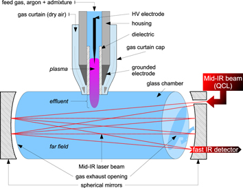
Figure 1. Sketch of the experimental setup illustrating the plasma source kinpen with the gas curtain cap connected with the diagnostic chamber of the QCL absorption setup located in a multipass cell.
Download figure:
Standard image High-resolution imageA feed gas flow rate ranging from 0.5 to 3.0 slm of dry argon can be blown through the capillary and after excitation produces a visual plasma outside the nozzle between 0.3 and 15 mm length. The plasma length depends on the admixture type and fraction. Typically,  and
and  can be admixed to the feed gas up to 2.0%. Also water vapour can be added to the feed gas in a smaller proportion (about 1400 ppm) to control the production of OH or hydrogen peroxide (
 ) in the plasma and its effluent [11, 25].
In order to control the interaction of the plasma and its effluent with the surrounding atmosphere, an external gas flux is implemented by means of a gas curtain device. More information can be found in [4]. This gas curtain can be fed with different gases, however, for the purpose of this work dry air is used, only to keep the ambient humidity out of the active region, as reported in [26]. Additionally, the gas curtain enhances the reproducibility and the stability by excluding any variation of water vapour concentration which strongly depends on the location and time of operation. Furthermore, this gas curtain device is used to couple the plasma jet with the measurement chamber providing a similar atmosphere near the plasma effluent as in open conditions.
2.2. Quantum cascade laser absorption spectroscopy (QCLAS) diagnostic technique
Absolute density measurements of  and
and  produced by the kinpen are performed by laser infrared absorption spectroscopy in the mid-infrared. The experimental setup is identical to the one we reported in previous work by Isni et al and which will be described briefly here [27].
The diagnostic apparatus is initially based on the Q-MACS system (neoplas control GmbH, Germany) although some optimizations were performed to allow investigations of plasma jets operating at atmospheric pressure [13, 27].
For the measurement of both species,  and
and  , a nanosecond single mode pulsed quantum cascade laser (QCL) is used as a mid-infrared source driven in inter-pulse mode [28, 29]. Unfortunately, pulsed QCLs have typically an emission range only within a few wavenumbers (about 5–15 cm−1), whereas both
  and
and  have their absorption bands separated with a gap of about 600 cm−1. Consequently, two different QCLs (Alpes Lasers SA, Switzerland) are used alternatively, emitting from 1607.72 to 1619.43 cm−1 and from 1024.5 to 1029.9 cm−1 to match the absorption band positions of
  and
and  respectively.
The intensity stability is enhanced by a Peltier element which permanently regulates the temperature. The tuning of the laser wavelength is performed by temperature variation induced by a fast current ramp. This method allows us to shift the laser wavelength over a range of 0.8 cm−1 in order to produce an absorption spectrum of many ro-vibrational transitions.
As the absorption properties of each molecule in the mid-infrared as well as the expected densities are rather low [30], a 60 cm multipass White cell is used in order to increase the absorption length. The laser beam is focused on the entrance of the multipass cell and is then reflected several times before reaching a very fast mercury cadmium telluride detector (Q-MACS IRDM-600A, neoplas control GmbH, Germany). The number of passes through the cell is tunable. In this work, a number of 32 passes and a total absorption length of 19.2 m is sufficient to observe a good absorption signal. The signal is acquired by a digitizer board controlled via a computer. The latter monitors the complete system by means of QMACSoft Monitor software [31].
Figure 1 illustrates the diagnostic bench and focuses on the coupling of the plasma source to the measurement chamber. In order to collect the reactive species produced by the plasma jet, a measurement chamber is mounted within the multipass cell. The chamber is a cylinder of 9.0 cm inner diameter and 57.5 cm length, yielding a volume of 3660 cm3. It is made of glass in order to prevent reactions with the wall and thus reduces chemical losses.
The coupling of the plasma jet to the measurement chamber is achieved by an opening located at the half-height of the cylinder at the centre of the multipass cell to conserve symmetry between the two exhausts. The gas curtain cap mounted on the plasma device helps to keep the connection with the chamber tightened. It also provides air around the plasma effluent to reproduce the ambient conditions and prevent the chamber to be filled with argon.
As shown in figure 1, the mid-IR beam is reflecting on the multipass cell mirrors and passes through the chamber without interaction with the active visual plasma itself. The homogeneity of the gas mixture within the chamber has been checked in a previous work and confirmed by a numerical CFD model [27].
The absolute density measured within the chamber is determined as follows: the laser is tuned to scan a range of about 0.8 cm−1 yielding the absorption spectrum. The latter is fitted with a simulated spectrum based on the line strength reported in the HITRAN database [30, 32]. The procedure is automatically implemented through the QMACSoft Monitor software and allows a sample rate of 0.5 Hz in our experimental conditions. The absolute wavelength position and wavelength scale distortion during the laser tuning are corrected via a calibration procedure reported in [13]. Herein, a more detailed description of the fitting method is given.
In order to dry the pipes and the measurement chamber, the gas curtain was flushed with 5.0 slm dry air, at least 12 h before to start. Similarly, the argon pipes were flushed in advance with 0.5 slm for over 6 h. Indeed, water is known to have many broad absorption bands in the mid-IR which can lead to a significant disturbance and to an over-estimation of the production rates (or concentrations) of the species but also because even very low amounts of water will influence the plasma chemistry [9, 11, 26]. Moreover, this protocol enhances the repeatability and stability of the diagnostic.
From the measured densities  of species
  , the net production rates
  :
:
are calculated accounting for the total gas flux of 8 slm, i.e. combined curtain gas and argon feed gas flux.
2.3. Power
The power dissipated at the electrode is one of the key parameters to determine how much energy excites the electrons and it is a crucial input parameter for the simulations (see below).
In this work, the power measurement is performed in the same way as reported by Hofmann et al [33]. The current and voltage probes (Tektronix Tek CT-2 and Tek P6139A respectively) are installed before the matching coil directly on the kinpen electronics. Thus, current and voltage are recorded simultaneously with an oscilloscope (Tektronix DPO 4104) and allow the determination of the average power dissipated by the HV electrode. Losses induced by the coil and wires are taken into account following the protocol suggested in [33].
This results in a measured dissipated power ranging from 1.4 to 1.8 W in the case of impurity admixtures up to 1.0%. These values of dissipated power are in agreement with the power reported by other groups using similar argon RF atmospheric pressure plasma jets, i.e. with similar length and gas temperatures, geometry, gas flow rate, etc [24, 34].
2.4. Gas temperature
The gas temperature value is a crucial parameter for the application as it needs to be close to room temperature (a few millimeters from the nozzle) in order to avoid any thermal damage on the sample. Moreover, it is also important to know the evolution of the temperature throughout the plasma to be able to accurately model the reaction chemistry.
The gas temperature is measured with a non-metallic fiber-optics probe (diameter 1 mm) mounted on a three-axis linear table. The device determines the temperature by spectroscopically measuring the band gap of a GaAs crystal deposited at the tip of the optical fiber (FOTEMP1-OEM and TS3, Optocon AG, Germany). Unlike for metallic probes, there is no visible change in the emission of the plasma when the probe is brought in contact with the visible plasma. However, it is noted that with the probe merely average temperatures can be detected, while in a turbulent flow the local temperature can be expected to exhibit significant statistical fluctuations.
2.5. Admixture variation
The kinpen in this work is operated with 3.0 slm argon (99.999% purity) gas feed flow rate and an additional gas curtain of 5.0 slm dry air. The gas flow is regulated by mass-flow controllers (MFC, MKS Instruments, USA). To prevent any impurities and ambient humidity from penetrating the pipes and contaminating the argon, stainless-steel and PTFE gas tubes are used [11].
In this work, an admixture variation of  and/or
  is applied from 0.0 to 1.0% of the total feed gas flow rate (0.0–30.0 sccm in absolute values, respectively). The purity is 99.995% for
  and 99.999% for
  according to the provider specifications (Air Liquide GmbH).
Additional water impurities may result from residual humidity in the tubing as well as diffusion through the tube walls. In the previous work [26] the resulting feed gas humidity was determined to be less than 20 ppm for this setup after flushing the tubes as specified in section 2.2. 1 ppm level water impurity in the feed gas was thus also included in the numerical model used in this work. Furthermore, the molecular admixtures  and
and  are expected to be much larger (0.1–1%) than the residual impurities from the gas bottles and the tubing and hence are expected to dominate the RONS chemistry.
The mixing of either of these molecular gases with argon is performed before the gas is blown through the plasma jet in order to obtain a better homogeneity. The admixture step is 0.1% (3.0 sccm) and controlled by calibrated mass-flow controllers.
Additionally, an artificial mixture of both  and
and  is also used in this work besides admixing both gases separately. Obviously, this should result again in a different gas composition of the plasma and the effluent. In this case, the argon/admixture ratio is fixed (Ar 99.0 + 1.0% admixture) but the content of the admixture fraction itself is varied from 0.0 to 100.0%
  with 100.0–0.0 %
  . Hence, a 0.2%
  /0.8%
/0.8%  ratio is equivalent to a 1.0% dry air/99.0% argon admixture.
2.6. Model description
The numerical simulations are performed with a 0D chemical kinetics model which is based on the original GlobalKin source code, developed by Kushner and co-workers [35]. Previously we developed a large Ar/N /O
/O /H
/H O reaction set of 85 species interacting by means of 302 electron impact reactions and 1626 heavy particle reactions. This extensive reaction set was presented previously [36] and for more details about this input data we refer to the supplementary information. This is necessary to calculate the densities of biomedically active species, which often have relatively low concentrations, within a broad parameter range. Some minor adjustments to the initial reaction set were reported by Van Gaens et al [9, 37].
Several modifications to the original code enable us to evaluate the species densities and chemical reaction pathways throughout the plasma jet propagating in an open humid air atmosphere. These modifications are thoroughly discussed in a previous paper [36], but the most important adjustments are briefly summarized below and in the appendix.
We assume that the active plasma species can be found within a cylindrical area along the plasma jet and its effluent, which has the same diameter as the inner diameter of the plasma jet tube. This area corresponds to the visual plasma jet and beyond (see figure 2). During the simulation, we track a cylinder segment that flows along the symmetry axis of the jet. The length of the segment is the distance that the gas travels within one time step of the calculations (order of μs ). Since our model is 0D the plasma properties (such as the species densities) are volumetrically averaged over this cylinder segment.
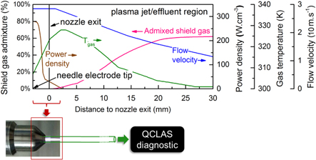
Figure 2. kinpen characteristics along the axial symmetry axis of the device. These profiles of the curtain gas diffusing into the argon feed gas stream, the power density, gas temperature and gas flow velocity are the input to our chemistry model and match either the experimental measurements or the fluid flow calculations (see text). The nozzle exit is located at the axial position of 0 mm. The powered needle electrode (and thus the highest power density) is located a few millimeters before this position. After the nozzle, the plasma jet can freely propagate and eventually enters the 'effluent' region when the power density has become zero and where the temperature drops to 300 K.
Download figure:
Standard image High-resolution imageThe plasma properties for this cylinder segment will change when it moves further along the flow because it is subjected to a varying power deposition, flow velocity, gas temperature and impurities diffusing from the gas curtain, as a function of its position.
It is very important to mention that these plasma parameters are not calculated self-consistently within our model.
The gas flow velocity and the gas curtain entrainment rate follow from an external 2D computational fluid dynamics simulation of the neutral gas at room temperature using Reynolds-averaged Navier–Stokes equations with a standard k– model to account for the turbulence [38]. At a gas flow rate of 3 slm and a corresponding Reynolds number of
  the flow is expected to be fully turbulent. The computed ambient species densities agree well with mass spectrometric measurements [38–40].
In the far effluent region the gas will eventually become stationary and there we assume that the 3 slm argon feed gas is fully mixed with the 5 slm dry air of the gas curtain. However, it is obvious that there is also an admixture gradient of the gas curtain in the radial direction of the jet. As our model is 0D without a degree of freedom in the radial direction, we simply tested which of the admixture profiles (from different off-axis positions) resulted in the best agreement between the simulations and the measurements. Eventually, the gas curtain admixture profile at r = 0.6 mm (determined by the 2D fluid dynamics simulations) resulted in the best correspondence between the experimental and the calculated species densities. Due to this approximation some effects related to multiple dimensions might be neglected. In reality the situation is more complex as the propagation of the ionization wave is strongly linked to the turbulent flow pattern. It was recently found that the ionization wave preferentially propagates through the channel with the highest noble gas content and thus the lowest concentration of admixtures (in the order of 1% and lower)[39]. Moreover, as the ionization wave follows the vortices occurring in the turbulent flow, it is often positioned off-axis [41].
The power deposition profile within the device and the visual plasma obviously depends on the electric field generated by the electrodes and the plasma itself. It is greatly affected by the electrode setup, as was already demonstrated by this model in a previous work [9]. Because the electrode configuration of the kinpen has a very similar geometry, we use the same shape for the power deposition profile (see figure 2) but the magnitude of the power density is scaled down to match the operating conditions of the kinpen; we set the total power deposition equal to 1.5 W (see section 2.3). The power density determines in every timestep how much energy is transferred to the electrons in the electron energy equation.
Important is also that our power deposition profile shown in figure 2 does not explicitly take the RF excitation waveform into account. We apply this simplification since we are primarily interested in the dynamics of long-lived species and therefore neglect fluctuations on the sub-microsecond timescale. Thus, it should be sufficiently accurate that the total deposited power for the calculations is equivalent to the experimentally measured plasma power deposition, as long as the bulk chemistry does not change by neglecting the RF excitation. Our previous work showed that this assumption is valid for argon plasma jets operating at a higher frequency of 13.56 MHz [9, 42].
The experimentally measured gas temperature profile is plotted in figure 2 as well. We directly used the on-axis probe measurement, i.e., maximum temperature values, as described above and did not account for the effect of a radial gradient in the temperature. The gas temperature value can influence reaction rates since the coefficients are a function of this parameter. Also note that the experimental measurement (see section 2.4) indicates that the gas temperature already starts decreasing at a few millimeters from the nozzle exit. However, within the apparatus the temperature could not be measured accurately (with spatial resolution) and therefore needed to be estimated.
In some of our previous work a temperature profile that starts rising (from room temperature) at the needle tip position was used as an input, assuming that the temperature rise is mainly caused by exothermic reactions of highly reactive radicals or highly energetic species created by electron impact processes. Indeed, when the temperature is calculated by the 0D model itself, these processes cause a maximal temperature value at the same position, shortly after the nozzle exit. Nevertheless, we opted not to adopt the calculated temperature profile because it is not consistent with the experimentally measured values further into the effluent. The deviation is probably related to turbulent heat transfer.
The main advantage of our 0D semi-empirical approach is the possibility to implement the large chemistry set of an Ar/N /O
/O /H
/H O mixture necessary to simulate the kinetics of the biomedical species (which are often not the main plasma components) without excessive calculation times, and while staying close to the experimental conditions.
Evidently, this model needs a good validation by thorough comparison with experimental measurements, as previously demonstrated in Zhang et al [42] and Van Gaens et al [9]. In the latter paper, a good correspondence with the measured NO and O densities was presented for a kHz pulsed RF driven argon plasma jet with air admixtures. In Zhang et al [42] a good quantitative agreement was obtained for the  density in an RF driven argon plasma jet with
  admixture. Note that in both studies this validation was done with spatial resolution along the symmetry axis of the jet.
3. Results and discussion
In this section the spectroscopically measured and numerically simulated O3 and NO2 net production rates in the far effluent of the plasma jet (measurement cell) are displayed and compared. In the following three subsections, this is done for  ,
,  or
or  +
+  admixtures, respectively. In each of these sections, we also present a detailed reaction kinetics analysis for both O3 and NO2 , as obtained from the model.
In the context of the comparison of these net production rates in the measurement cell (e.g. the values depicted in figure 3), it is important to mention that the model was previously only used for simulating the plasma jet and its effluent for a typical timescale of milliseconds. However, as the residence time of the plasma jet effluent within the measurement cell during sampling by the QCLAS is significantly longer (calculated to be around 25 s), we changed the end time for our simulations to 6 s, in order to allow for a correct comparison with the measured net production rates. At this point there are no drastic changes in the gas densities of O3 and NO2 anymore.

Figure 3. NO2 and O3 densities (left y-axis) or net production rates (right y-axis) after 25 s residence time in the measurement chamber as obtained by infrared absorption spectroscopy and the calculated data for a similar time scale (i.e. 6 s, after which the densities stay constant), for different N2 fractions added to the argon feed gas.
Download figure:
Standard image High-resolution imageAdditionally, it needs to be stressed that the values depicted in figure 3 (and similar figures below) are net production rates after 6 s residence time in the measurement chamber. This distinction has to be made in order to avoid any confusion with the values of figure 4 (and the consecutive similar figures) which represent the ongoing chemistry within a cylinder segment travelling within the plasma jet device, the active (visual) plasma jet and a first part of the effluent (i.e. a total of 10 ms). Also note that production and loss rates are presented separately in this type of graph unlike the net production rate shown in figure 3.

Figure 4. O3 chemistry inside the device, the plasma jet and the initial effluent (10 ms in total), as a function of the N2 admixture. Top graph: the white dots represent the total production/loss rates (cm s
s , left y-axis); the colour areas (linked to the right y-axis) represent for each region the spatially averaged relative contributions of the dominant reactions to the total production/loss. The production is plotted in the upper half and the loss in the lower half of the top graph. Note that the y-axis of the loss rates increases from top to bottom, hence opposite to the y-axis of the production rates, to clearly indicate their opposite effect. Bottom graph: spatially averaged O3 densities in the three regions as a function of the N2 admixture.
Download figure:
Standard image High-resolution image3.1. Nitrogen admixtures
Figure 3 (top) demonstrates a very good agreement between the experimentally measured and simulated NO2 production rate, for the investigated range of  admixtures between 0 and 1%: the trend as a function of the N2 admixture and the absolute values are very similar, with at maximum a factor 2 difference for 0% N2 . Unfortunately, this is not the case for the O3 production rate where the difference is up to a factor 3 (see figure 3 (bottom)). Furthermore, the model predicts a steeply increasing O3 production rate between 0 and 0.2% admixed N2 , whereas the experiments indicate only a very slight increase over the entire operating range. Note that this might be explained by the fact that these
  concentrations are near the detection limit of the diagnostic setup under the present experimental conditions. Moreover, experimentally, very slight differences in the jet properties, such as turbulence or impurities in the tubes, can easily occur. This determines the concentration of molecular gases in the argon and therefore indirectly affects the O3 concentrations. Indeed, we will show in this paper that the balance between production and loss rates is often very delicate and that a slight inaccuracy can have a large influence on the NO2 and O3 net production rate. In this context it needs to be mentioned that we chose to keep the gas curtain entrainment rate consistent for all the simulations, so for the different admixture amounts and for the different admixture gases.
We will now further clarify the production pathways of O3 and NO2 by means of a detailed chemical analysis, as obtained from the model, but now focussing mainly on the chemistry that occurs on the time scale of milliseconds. Indeed, this is the time frame where, chemically speaking, the most interesting changes happen. Obviously, this time frame corresponds to the distance that a gas element travels within the kinpen device, the active/visual plasma jet and finally the initial effluent region (thus not the entire measurement cell). The displayed values in figure 4–9 below (i.e. density, the total production and loss rates, the relative contributions of the reactions and electron temperature) are averages for one of these three regions, obtained by performing an integration along the symmetry axis of the jet. Accordingly, the most important chemical phenomena can be identified for each region.
For example, the density evolution of a species, from the vicinity of the needle electrode tip until the early effluent, is thus reduced to only three data points. Indeed, this turned out to be crucial for maintaining a relatively simple overview of the changing chemistry when varying the admixture ratios and at different distances from the nozzle and the needle tip. To make this concept easier to interpret, we added the schematic of the plasma jet above the reaction kinetics data in figure 4.
Also important is that in each figure the production rates are displayed in the upper part of the top graph and the loss rates in the bottom part of the top graph (both with white dots, left axis). Note that the y-axis of the loss rates increases from top to bottom, hence opposite to the y-axis of the production rates, to clearly indicate their opposite effect. The same top graph also displays the contribution of the different reactions to the total production and loss rates by colour areas (right axis). We only show the reactions which contribute more than 10% to the total loss or production of a species. Note that we show all these contributions, for the sake of completeness, but in the text we only discuss the most important production and loss processes. Therefore, the sum of the different contributions often does not reach the full 100%. The most important processes are indicated in bold in the legends at the right of the graphs. The bottom graph of these figures presents the species densities.
The short time-scale information in these plots (e.g. Figure 4) is, in general, sufficient to explain the trend observed on the longer time-scale (see figure 3).
3.1.1. O3 formation
Figure 4 illustrates that  is mainly formed in the effluent region (see white dots in the top graph) for all N2 admixtures investigated. Indeed, the formation rate in the plasma jet is about one order of magnitude lower, and there is no
  formation at all inside the device. The figure shows the following dominant pathway:

It is clear from figure 4 that the production rate in the effluent region is more than two orders of magnitude higher than the loss rate (see upper and lower part of the top graph). Indeed, the main species responsible for the loss of  are the electronically excited states
  (a) and
  (b) (see figure 4 as well), but they do not reach sufficiently high concentrations. The
  density as a function of the N2 admixture in the early effluent therefore corresponds to the production rate in the far effluent as predicted by the model and depicted in figure 3 (note the logarithmic scale in figure 4). Recall, however, that the agreement with the experimental result was not very good in this case.
As the O atoms are fully responsible for the  production, we will now analyze the chemistry of this species.
Figure 5 illustrates that the variation of the O density as a function of the  admixture is very similar to that of O
 . Furthermore, it can be seen that the O atom production occurs mainly in the plasma jet region. Indeed, in this region
  from the gas curtain starts to diffuse into the argon jet, as shown in [39, 40, 43].
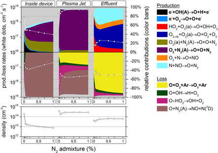
Figure 5. O chemistry inside the device, the plasma jet and the initial effluent (10 ms in total) as a function of the N2 admixture (see figure 4 for an explanation about the top and bottom graph).
Download figure:
Standard image High-resolution imageYet for 0% N2 admixture, the O atom production inside the device is quite significant. Indeed, there is only some N2 present in the form of impurities, because, as initial conditions of our simulations, we always impose a slight amount of N2 , O and H
and H O in the argon feed gas (1 ppm) to mimic the impurities in the gas bottles and desorbed molecules from the piping. This N2 impurity level is insufficient to reduce the electron temperature as drastically as for cases with significant N2 fractions (see figure 6), where a lot of energy is used for vibrational excitation of N2 . Fast electron impact dissociation of O
 and electronically excited OH radicals, i.e. OH(A) created from H
 O, are therefore possible within the kinpen device at 0% N2


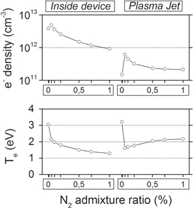
Figure 6. Spatially averaged electron densities  ) and average electron temperature (eV) inside the device and in the plasma jet, as a function of the N2 admixture. The effluent region is not shown, as the electrons will be negligible in this region.
Download figure:
Standard image High-resolution imageAs a result, the O atom density is already significant within the kinpen device when no  is admixed to the argon.
This also explains the maximum in the O atom density in the plasma jet region, at 0% N2 , and the clear drop upon addition of small N2 admixtures. However, at larger N2 admixtures the O atom density increases again. Here, the O atoms are mainly created from collisions of  species with the nitrogen metastable (N2 (A)):

Moreover, in the plasma jet region the rates of the reactions (2) and (3) become insignificant for 0%  . This is because the electron density drastically drops as a result of electron attachment to oxygen species (see figure 6; note that the electron chemistry itself is, however, not explicitly shown in this paper) since the
  density quickly rises due to the mixing of curtain gas with the argon.
Note that figure 7 illustrates that  is also significantly quenched in this region but the quenching of this state is much slower than that of the electrons. Additionally, the rising
  density compensates for this
  quenching and still causes the rate of reaction (4) to be high in the plasma jet region.

Figure 7. N2 (A) chemistry inside the device, the plasma jet and the initial effluent (10 ms in total) as a function of the N2 admixture (see figure 4 for an explanation about the top and bottom graph).
Download figure:
Standard image High-resolution imageBesides, figure 7 also illustrates that N2 (A) is mainly formed inside the kinpen device, i.e. by electron impact excitation of ground state N2 :

Thus one might expect a rising N2 (A) density upon increasing N2 admixture, simply because the density of one of the reactants becomes higher.
However, above 0.4% N2 the electron density and electron temperature, plotted in figure 6, become quite low (due to the vibrational kinetics, as mentioned above) and this compensates for the rising N2 density. This even causes a slight drop in the rate of reaction (5) above 0.4% N2 and the same behavior is therefore seen for the N2 (A) density in the bottom graph of figure 7. As a result the rate of reaction (4) (causing the dissociation of O into O atoms in the plasma jet) will also first increase upon increasing N2 fraction (after the initial drop, as explained above), but after 0.2% N2 it will remain more or less constant (see figure 5). This explains the behaviour of the O atom density upon rising N2 fraction, and because the O atoms are mainly responsible for the O3 production, this also clarifies why the O3 production and O3 density first increase upon rising N2 fraction, then remains more or less constant and eventually slightly decreases for N2 fractions above 0.5% (see figure 4 and also figure 3 above).
The above explains the production rates predicted by the model. We believe that we at least identified all the dominant reactions correctly, although the agreement with the experiments is not perfect. Note that deviations can easily occur since the balance between the production and loss processes of all the species involved here is delicate. A more complete model approach might be better in this case.
3.1.2. NO2 formation
Figure 8 illustrates the NO2 production and loss rates, as well as the relative contributions of the different processes and the NO2 density, as a function of N2 admixture. It is clear that NO2 is mainly produced from NO, especially by reaction (6), and to a lower extent also by reaction (7):


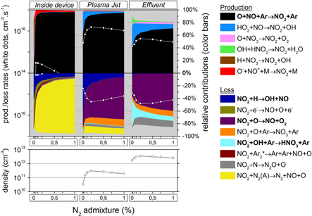
Figure 8. NO2 chemistry inside the device, the plasma jet and the initial effluent (10 ms in total) as a function of the N2 admixture (see figure 4 for an explanation about the top and bottom graph).
Download figure:
Standard image High-resolution imageThese processes are especially important in the plasma jet. Indeed, the total production rate of NO2 is almost an order of magnitude larger than the total loss rate here. In the effluent region this production rate has already decreased by at least a factor 2, but additionally the loss rate (i.e. mainly the reaction  ) is now of about the same magnitude. The net production rate is therefore much smaller in the effluent than in the plasma jet region.
Still, NO2 is a rather long-lived species because there are no highly reactive species present in the effluent that are sufficiently abundant to cause considerable NO2 loss within these time scales. Note that the O atoms are involved both in the main production and loss reactions of NO2 and this species will eventually get depleted in the effluent region (see figure 5 above. The same is true for N, OH and HO , which are involved in several other loss processes).
Important to mention is that NO2 reaches only its maximum concentration towards the end of the plasma jet region, whereas the density practically does not change any more in the effluent region and stays continuously high here. The averaging we performed thus results in a relatively low NO2 density in the plasma jet region, although it is mainly produced here.
Because NO is the main NO2 precursor, we show the NO chemistry in figure 9. NO is produced in large amounts early in the plasma jet region, by a reaction between N2 (A) and O atoms:

The reason for this is twofold: first, the maximum N2 (A) density is located close to the needle electrode where the power density is at maximum; further in the plasma jet it is rapidly quenched by  , thereby creating O atoms or excited
  molecules (see figure 7). Second, the O atoms only reach a maximum density in the plasma jet region, as illustrated in figure 5, because of the oxygen entrainment from the ambient into the argon, which obviously only starts after the nozzle exit. The combination of these two effects explains why the maximum rate of reaction (8) is located in the early plasma jet, close to the nozzle exit. Nevertheless, the production of NO by this reaction is also non-negligible inside the device, as is clear from figure 9.
As the excited N2 (A) molecules mainly determine the NO formation, and NO is the dominant NO2 precursor, the NO2 production as a function of the N2 admixture therefore largely follows the trend of the N2 (A) state, which depends both on the N2 fraction and on the electron temperature inside the kinpen device, as the latter determines the rate coefficient. Because the electron temperature (and hence the rate coefficient) drastically decreases upon increasing N2 fraction, at least within the device (see figure 6 above), these two effects are opposite to each other.
Thus, the NO2 production (and density) steeply rises immediately when small amounts of N2 are added, but beyond 0.15% N2 the NO2 production (and density) drops again, because the effect of the electron temperature starts to play a more dominant role. Indeed, this explains the trend seen for the NO2 production rate in figure 3 above.
3.2. Oxygen admixtures
This subsection is structured in exactly the same way as the previous one for nitrogen admixtures. We first look at the longer timescale, comparing experiments with simulations and consequently we explain the observed trends on the basis of a chemical reaction analysis of the short timescale.
The trends of both the NO2 and the O3 production rate as a function of the O fraction in the argon feed gas (from 0 and 1%) are reproduced well by the model, as demonstrated in figure 10. The NO2 production rate decays exponentially as a function of the O
 fraction, while the O3 trend is practically the inverse with a sharp increase between 0 and 0.2%
  . The absolute values are, however, not fully comparable, although the difference is at most one order of magnitude within the investigated range of the
  fraction. As previously stated, this might be related to the inaccuracy on the amounts of curtain gas that diffuses into the jet (i.e. the absence of a radial gradient in the model or consequences of turbulence).
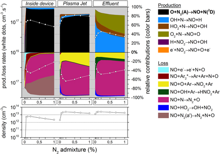
Figure 9. NO chemistry inside the device, the plasma jet and the initial effluent (10 ms in total) as a function of the N2 admixture (see figure 4 for an explanation about the top and bottom graph).
Download figure:
Standard image High-resolution image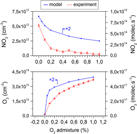
Figure 10. NO2 and O3 densities (left y-axis) or net production rates (right y-axis) after 25 s residence time in the measurement chamber as obtained by infrared absorption spectroscopy and the calculated data for a similar timescale (i.e. 6 s, after which the densities stay constant), for different O fractions added to the argon feed gas.
Download figure:
Standard image High-resolution image3.2.1. O3 formation
As described in section 3.1.1,  is almost exclusively produced by reaction 1. However, in the case of adding
  , this occurs already in the plasma jet region and even inside the device, at least for
  fractions above 0.2%, as demonstrated in figure 11.

Figure 11. O3 chemistry inside the device, the plasma jet and the initial effluent (10 ms in total) as a function of the O admixture (see figure 4 for an explanation about the top and bottom graph).
Download figure:
Standard image High-resolution imageFor lower  levels there is clearly not yet enough O
 present inside the device and in the (early) plasma jet to yield a large rate for reaction (1). Therefore, the production will occur in such a case mainly in the effluent region when there is enough diffusion of O
 from the gas curtain.
At higher O fractions, the production of O3 is smaller in the effluent than in the plasma jet region or even inside the device. Nevertheless, since the O3 loss is clearly negligible in the effluent region, the O3 density is still at maximum here (see figure 11). This explains why O3 is a relative long-lived species. As described in section 3.1.1, the O3 production is mainly determined by the O atoms; therefore, the chemistry of the O atoms is displayed in figure 12. The O chemistry, however, is now considerably different from the case when adding
  (section 3.1.1). Indeed, the O atoms are now mainly produced within the kinpen device, so mainly from the oxygen admixture itself and not from the gas curtain.
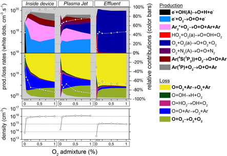
Figure 12. O chemistry inside the device, the plasma jet and the initial effluent (10 ms in total) as a function of the O admixture (see figure 4 for an explanation about the top and bottom graph).
Download figure:
Standard image High-resolution imageSecondly, in the absence of significant  admixtures, the O atom production is now mainly due to the dissociation of
  by direct electron impact and by collisions with energetic argon species (i.e. Ar
 excimers, Ar(
 S(
S( P
P )) metastables, as well as higher excited states, grouped in the model as Ar(
 P), but not by collisions with N2 (A). Note that the heavy particle reactions with energetic argon species are in fact also an (indirect) result of electron impact reactions, because these species are created by electron impact excitation of Ar ground state atoms, possibly followed by an association with another Ar atom to form the Ar
 excimers (data not shown).
A third difference is that the contribution of  dissociation upon collisions with the argon species increases with rising
  fraction, whereas the contribution of direct electron impact dissociation drops (at least between 0 and 0.2%
  ). Indeed, the contribution of the latter process is more than 60% at very small
  concentrations, compared to about 30% above 0.2%
  . This can be explained by the electron temperature evolution as a function of the
  admixture (see figure 13). Clearly, the average electron temperature rises for higher
  admixtures and argon excitation therefore becomes relatively more important than
  dissociation because of the higher threshold energy and since the reaction coefficient thus drastically increases with the electron temperature.
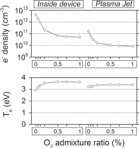
Figure 13. Spatially averaged electron densities (cm ) and average electron temperature (eV) inside the device and in the plasma jet, as a function of the O
 admixture. The effluent region is not shown, as the electrons will be negligible in this region.
Download figure:
Standard image High-resolution imageFinally, note that after the initial rise in net O atom production (and thus O atom density) until 0.2% O , the O atom density stays relatively constant at higher O
 admixtures (i.e. between 0.2 and 1.0% O
 ). This is not only because the average electron temperature is rather constant in this range but also because the O atoms seem to be 'self-quenching' as the main loss pathway of the O atoms creates
  (see reaction (1)) and the latter is also quite important for the loss of O atoms (see figure 12 again):

The  production is therefore almost linearly dependent on the O
 fraction between 0.2 and 1.0% (or between 0.3 and 1.0% for the experimental values), as was depicted in figure 10. Indeed, the rate of reaction (1) is practically first order because the O atom concentration does not change much in this range.
3.2.2. NO2 formation
The admixture of  does not change the dominant production pathway for NO2 compared to the admixture of
  (see section 3.1.2). NO2 is still mainly formed by the reaction between O and N2 (A) producing NO (by reaction (8) above, data not shown again here), which then oxidises further by the three-body reaction with O atom and Ar as the third collision partner (see reaction (6) above), as depicted in figure 14.

Figure 14. NO2 chemistry inside the device, the plasma jet and the initial effluent (10 ms in total) as a function of the O admixture (see figure 4 for an explanation about the top and bottom graph).
Download figure:
Standard image High-resolution imageThe net production rate is the highest towards the end of the plasma jet region (the loss is significantly lower than the production although this is difficult to see due to the log scale). Note that some NO2 production also occurs in the effluent region but the loss rate is now more comparable to the production rate here. However, the NO2 density shown in figure 14 is not as high in the plasma jet region as in effluent region, again simply due to the averaging (as explained above).
The NO2 formation once more depends indirectly on the N2 (A) formation and this species is produced less upon increasing  admixture (see figure 15). This is because N2 (A) is mainly formed from electron impact excitation, as can be seen from this figure, and the density of the electrons, which are involved in this reaction, rapidly drops when increasing the
  content (see figure 13). The latter is caused by efficient electron attachment processes for
  species. Obviously, the reaction rate of electron impact excitation (reaction (5)) also depends on the electron temperature which determines the rate coefficient, but this is less important in this range of electron temperatures (3–3.5 eV). Therefore, the production of N2 (A), as well as the N2 (A) density, clearly drop upon increasing O
 fraction, as shown in figure 15.

Figure 15. N2 (A) chemistry inside the device, the plasma jet and the initial effluent (10 ms in total) as a function of the O admixture (see figure 4 for an explanation about the top and bottom graph).
Download figure:
Standard image High-resolution imageSecondly, the NO2 formation also depends on the concentration of the other reactant, i.e. the O atoms. The density of this species drastically rises when very small amounts of  are added to the feed gas, but afterwards (beyond 0.1%) the density remains more or less constant, as discussed above (see figure 12).
Combining the N2 (A) and the O density trends upon increasing  admixture indeed leads to the observed behaviour of the NO2 density as a function of the O
 fraction, depicted in figure 14: a steep rise between 0 and 0.1% O
 to a maximum of about 10
 cm
cm followed by a clear drop for higher O
 fractions.
Note, however, that the calculated and measured net NO2 production rates as a function of the O admixture, illustrated in figure 10 above, do not exhibit this initial rise between 0 and 0.1% O
 , that is observed in figure 14 (not only for the NO2 density, but also for the NO2 production rate). The reason is that the calculated and measured NO2 net production rates, shown in figure 10 above, apply to a much longer time scale (i.e. in the order of seconds; see the total residence time in the measurement cell, as described at the beginning of section 3), whereas the calculation results of the effluent region depicted in figure 14, apply to a time scale in the order of milliseconds.
Within this shorter time frame, the loss of NO2 occurs predominantly by collision with O atoms, and these species will eventually disappear from the discharge (for example by forming O3 as described above). Therefore, in a later stage of the effluent, O3 will be the only available molecule able to react with NO2 as it is the only reactive species that is at least as abundant as NO2 . Note that the reaction NO2 + O3 is not displayed in figure 14 because only the dominant reactions contributing more than 10% are presented, but at longer residence times, this reaction eventually becomes important. As the O3 density is rather small for O admixtures between 0 and 0.1%, the NO2 loss at these longer time scales will also be negligible at these low O
 admixtures. Therefore the net production of NO2 will be higher between 0 and 0.1% at these longer time scales, and indeed the NO2 net production rate will continuously drop from 0 to 1% O
 as illustrated in figure 10 above.
3.3. Oxygen+nitrogen admixtures
An interesting combination of the two chemistries clarified in the previous sections is obtained when  and
and  are simultaneously added to the argon feed gas. Recall that in this case, a fixed 1% O
 + N2 admixture is used, but with the O
 /(O
/(O + N2 ) ratio varied between 0 and 100%. Therefore, 0% O
 /(O
/(O  + N2 ) in figures 17–21 correspond to the conditions of 1% N2 admixture in figures 4–9, whereas 100% O
 /(O
/(O  + N2 ) corresponds to the case of 1% O
 in figures 11–15.
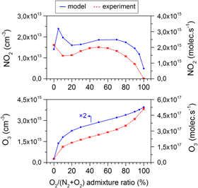
Figure 16. NO2 and O3 densities (left y-axis) or net production rates (right y-axis) after 25 s residence time in the measurement chamber as obtained by infrared absorption spectroscopy and the calculated data for a similar time scale (i.e. 6 s, after which the densities stay constant), in different O /(O
/(O + N2 ) ratios.
Download figure:
Standard image High-resolution image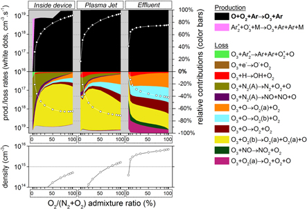
Figure 17. O3 chemistry inside the device, the plasma jet and the initial effluent (10 ms in total) as a function of the O + N2 admixture (see figure 4 for an explanation about the top and bottom graph).
Download figure:
Standard image High-resolution image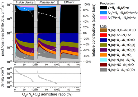
Figure 18. N2 (A) chemistry inside the device, the plasma jet and the initial effluent (10 ms in total) as a function of the O + N2 admixture (see figure 4 for an explanation about the top and bottom graph).
Download figure:
Standard image High-resolution image
Figure 19. O chemistry inside the device, the plasma jet and the initial effluent (10 ms in total) as a function of the O +N
+N admixture (see figure 4 for an explanation about the top and bottom graph).
Download figure:
Standard image High-resolution image
Figure 20. NO chemistry inside the device, the plasma jet and the initial effluent (10 ms in total) as a function of the O + N2 admixture (see figure 4 for an explanation about the top and bottom graph).
Download figure:
Standard image High-resolution image
Figure 21. N chemistry inside the device, the plasma jet and the initial effluent (10 ms in total) as a function of the O + N2 admixture (see figure 4 for an explanation about the top and bottom graph).
Download figure:
Standard image High-resolution image
Figure 16 illustrates that the simulated evolution of the NO2 and O3 net production rates is also well in accordance with the measurements. For both species, the shape of the curve is quite complex. The NO2 production rate initially drops (except for a first rise between 0 and 5% O for the model results), but increases again at about 20% O
 /(N2 + O
 ). A second maximum is formed at about 50% O
 /(N2 + O
 ) before the production rate steeply drops close to 100% O
 (thus for low N2 levels).
The shape of the O3 production rate as a function of the admixture composition is clearly x
 -shaped, although more pronounced in the experimental measurements. Indeed, the difference between the simulated and measured O3 production rate is in general about a factor 2, but in the middle of the investigated range, at an O
 /N2 ratio close to 1, this difference has increased to a factor 3.
3.3.1. O3 formation
The  formation pathway was found to be similar for O
 or N2 admixtures, as demonstrated above. Therefore, figure 17 indicates that the same mechanisms are applicable here when admixing both gases at the same time, i.e. the formation is mainly due to the three-body reaction between O atoms and O
 molecules, with Ar as third body (see reaction (1)).
Again, like in the case of O addition, the production is highest in either the plasma jet (and inside the device) or very early in the effluent region, depending on the O
 content, as explained in section 3.2.1 above.
A dissimilarity between figures 10 and 16 concerning the net O3 production rate as a function of the O fraction is that for pure O
 admixtures the net production rate first rapidly rises (between 0 and 0.2% O
 in argon) but it tends to saturate at higher O
 concentrations (see figure 10), whereas for O
 + N2 admixtures (see figure 16) the first rise (between 0 and 0.2% in argon) is less steep and is followed by a gradual rise (between 0.2 and 0.8% O
 in argon) and, finally, a more drastic increase between 0.8 and 1% O
 in argon (which is more pronounced in the experimental data). The
  production without N2 (for pure O
 admixtures) is thus higher between 0 and 0.8% O
 than with N2 (in the case of O
 + N2 admixtures).
Indeed, the observed effect must be explained by the role of N2 (A) (which is created from the N2 admixture molecules in reaction (5), see figure 18) in the generation of O atoms, which eventually leads to O3 production by reaction 1. This O chemistry is illustrated in figure 19.
As demonstrated in section 3.1.1 above, the O atoms can easily be formed by reaction (4) (i.e. between N2 (A) and O molecules) when significant amounts of N2 are present. Indeed, figure 19 illustrates that this reaction gains importance when the O
 /(O
/(O + N2 ) ratio drops and it takes over the role of O
 dissociation by collision with argon species and by electron impact as the most important O atom production process.
Consequently, the N2 (A) chemistry in figure 18 provides the final answer. The increase in N2 (A) density upon decreasing O fraction in the plasma jet region is not linear between 100 and 0% O
 /(O
/(O + N2 ) (looking from right to left on the x-axis). Indeed, the N2 (A) density seems to be somewhat suppressed until 10% O
 /(O
/(O + N2 ), yet for even lower O
 /(O
/(O + N2 ) fractions than 10% the N2 (A) density will finally increase drastically.
It is clear from the loss reactions in figure 18 that even small amounts of O (above 0.1% O
 /(O
/(O + N2 )) efficiently quench the N2 (A) molecules, not only by chemical quenching leading to O atoms and thus O3 formation, but also by physical quenching. Thus, it can be concluded that the O3 production is partially inhibited when significant amounts of O
 and N2 are added simultaneously, explaining why the rise in the net O3 production is higher between 80 and 100% O
 /(O
/(O + N2 ) than between 20 and 80% O
 /(O
/(O + N2 ), as depicted in figure 16 above.
3.3.2. NO2 formation
For the NO2 production rate as a function of the O /(O
/(O + N2 ) admixture ratio one might expect the highest value for equivalent O
 and N2 fractions, but this does not seem to be the case (see figure 16 above). From the above sections, we know that NO2 is formed from NO and this is also valid here (therefore, the NO2 chemistry is not explicitly shown, as it does not give new information). Thus, by studying the chemistry of NO in figure 20 it is possible to explain the observed trend for the net NO2 production rate displayed in figure 16.
In the plasma jet region the NO density is, as expected, the highest between 10 and 70% O /(O
/(O + N2 ) ratio. However, in the effluent region a small dip at 20% starts to develop. This is due to significant NO destruction upon collision with N atoms:

Indeed, the concentration of the N atoms is at maximum at this O /(O
/(O + N2 ) ratio, as demonstrated by figure 21.
As a result, the measured and modelled net NO2 production rate further in the measurement cell (shown in figure 16 above) exhibits a similar profile as the NO density in the effluent region of figure 20, because NO2 is created from NO.
4. Conclusions
In this work we presented the results of both a semi-empirical numerical model, which describes the chemical kinetics within the kinpen plasma jet device (with a surrounding dry air gas curtain), and experimental measurements of the jet (far) effluent by high resolution QCL infrared absorption spectroscopy. The net production rates of the biomedical species,  and
and  , were determined with both techniques for multiple different operating conditions.
In the first two cases either  or
or  is admixed from 0 to 1.0% of the total argon feed gas flow rate. Additionally, an artificial mixture of
  +
+  is used and in this case, the admixture fraction is fixed at 1% but its content is varied from 0 to 100%
  with 100–0 %
  .
.
We obtained a good qualitative agreement in all cases for the net production rates of  as a function of the different admixtures. Concerning
  , the similarity of the results computed in the model and the experimental data is qualitatively correct for most of the investigated conditions. Nevertheless, in case of
  admixtures, a mismatch between the calculation and the measurement is observed. It is not clear whether this is caused by a possible inaccuracy in the reaction set or due to the gas curtain diffusion profile assumed in our 0D model, which is much more complex in reality [39]. In the latter case, a more sophisticated model approach might offer a solution.
Quantitatively, the results of both techniques do not vary by more than a factor three at maximum within the investigated range (i.e. a consistent overestimation compared to the experimental measurements). The highest  production rate was achieved at the highest investigated
  admixture of 1%, see figures 10 and 16 (i.e. 4.9×10
 molec s
 measured and 1.0 × 10
 molec s
 simulated). These figures also illustrate that the
  production initially drops steeply when
  is being replaced by
  (between 100 and 80% O
 /N2 + O
 ) while the decrease is much more gradual between 1 and 0.3% pure
  admixtures.
For the net production rate of  in the case of
  and
and  +
+  the agreement is almost perfect. It is remarkable that the calculated NO2 production rate is quite comparable to the measured results within the investigated ranges of pure N2 admixtures and N2 + O
 admixtures, i.e. between 1 × 10
 and 3 × 10
 molec s
 . Moreover, in both cases the NO2 production rate becomes significantly lower when the
  fraction is lower than 0.1% in the argon gas, see figures 3 and 16.
Due to the complementarity of the two distinct techniques that have been used, we have acquired important insight in the reaction kinetics in all regions of the kinpen device, even in areas that are not accessible by optical diagnostics. The pathways for the formation of  and
and  are quite complex. From the analysis of the model output, it is demonstrated that the production of
  and
and  is mostly triggered by two common species: atomic oxygen (O) as well as metastables of nitrogen (
 ), which are both energy carriers and lead to the formation and/or destruction of
  and
and  . O and
  , among other species like Ar metastables, can be considered as transient particles that are direct results of the electron chemistry and eventually lead to the formation of longer living molecules outside the kinpen device.
Even more important is that admixture differences, even at these relatively low levels, can significantly alter the electron density and temperature and therefore have a large impact on the chemistry. In general, it can be concluded that the production of these important biomedically active species can be manipulated by up to one order of magnitude by varying the amount of admixture or the admixture type. Based on these results, the feed gas and also the gas curtain composition can be selected even more carefully to optimize the applications.
Acknowledgments
The simulations were carried out using the Turing HPC infrastructure of the CalcUA core facility of the University of Antwerp, a division of the Flemish Supercomputer Center VSC, partially funded by the Hercules Foundation of the Flemish Government (department EWI). Furthermore, we are very grateful to Professor Mark Kushner for providing the original numerical code that is used as a basis for our simulations. Sincere gratitude is expressed towards Dr Andrei V Pipa for the discussions and knowledge about IR absorption spectroscopy, and to Dipl. Ing. Henrik Zimmermann and Dipl. Ing. Sven Glitsch for their expertise about QCLAS. François Riberi is acknowledged for assistance during the measurement campaign. Dr Jörn Winter is gratefully acknowledged for the fruitful discussions. The Institute for the Promotion of Innovation by Science and Technology in Flanders (IWT Flanders) is acknowledged for providing financial support to WVG. ASB, SI and SR gratefully acknowledge the funding by the Federal German Ministry of Education and Research (BMBF, grant #03Z2DN12).
Appendix
In this appendix we describe the features of the numerical model, as already described in our previous work [9, 36, 37].
Pseudo-one-dimensional plug flow
By using a 'pseudo-one-dimensional plug flow' approximation in this 0D model, it is possible to represent the time dependent evolution of species densities (as is typically the case in a 0D model) as a spatial dependence, hence, as a function of the position in the plasma jet device and effluent. This approach was previously successfully applied in [44] for a He/O discharge. We assume that the tube of the plasma jet device, the plasma jet itself and the initial effluent can be represented by a long cylinder, where constant atmospheric pressure conditions rule. The magnitude of the flow velocity determines the change of position of a volume averaged (0D) plug flow element, i.e. a cylindrical segment, along the jet stream. In our approach, we assume that axial transport of mass and energy due to drift and concentration gradients is negligible in comparison to axial transport by convection. Furthermore, no species transport in the radial direction is considered in this approach. Due to the very high axial flow speed (typically in the order of 10
 cm s
cm s ) compared to the radial flow speed, this seems acceptable for the first few cm's after the nozzle exit. We want to stress once more that the original dependency in our 0D model is density versus time and that the distance dependency is not an extra dimension solved by the equations.
Evidently, the flow velocity should decrease along the jet symmetry axis. This is due to gas expansion and obstruction by the relatively stationary surrounding atmosphere. Therefore, the gas flow velocity was fitted to the fluid dynamics simulation results, only considering neutral gas species, thus electric field forces of the plasma have no influence on the flow field calculation.
The relation between the time scale and the length scale is thus not simply the initial velocity at the nozzle exit as a constant factor but the time correlates with position through the variable flow speed, i.e. a nonlinear decreasing value along the jet effluent obtained from the 2D fluid model. An average of several velocity profiles over the radial direction (which are known from our 2D computational fluid dynamics simulation, as mentioned in the paper) is used for this purpose, which thus includes both the high and low flow speeds in the jet. The velocity is a nonlinear decreasing value along the jet axis.
Species continuity equation
The following continuity equation is solved for all plasma species included in the model (see tables A1 and A2 ):
where ni is the density of species i, aijR and aijL are the right-hand side and left-hand side stoichiometric coefficients of species i in reaction j, kj is the reaction rate coefficient and nlL is the density of the lth species in the left-hand side of reaction j. All these coefficients are input values, obtained from literature, according to a predefined reaction scheme (see supplemenatry information, available at stacks.iop.org/njp/17/033003/mmedia). Note that each new time step dt describes the length of the next volume averaged segment of the plug flow cylinder. In addition, since fluid dynamics are not included in this 0D model, the humid air diffusion (from the surroundings into the argon flow) is handled by adding a production/loss term,  , for Ar, N
 , O
, O and H
and H O. This makes that argon is gradually being replaced by a humid air mixture starting from the nozzle exit. Of course, these artificial source terms will vary along the jet effluent. We considered several diffusion profiles for different off-axis positions (as determined by the 2D computational fluid dynamics simulations) and we adopted the r = 0.6 cm off-axis values as they resulted in the best agreement with the experimental results. Effects related to multiple dimensions are therefore neglected by our model approach.
Table A1. Plasma species included in the model.
| Ground state neutrals | Excited state neutrals | Charged species |
|---|---|---|
| Ar | Ar( S[ S[ P P ]), Ar( ]), Ar( S[ S[ P P ]), Ar( ]), Ar( S[ S[ P P ]), Ar( ]), Ar( S[ S[ P P ]), Ar( ]), Ar( P)a , Ar P)a , Ar (a (a ) ) |
e
 , Ar , Ar , Ar , Ar , ArH , ArH
|
N, N |
N( D), N D), N , N , N  , N , N (A (A ),N ),N (a' (a' ) ) |
N , N , N , N , N , N , N |
O, O , O , O
|
O( D), O D), O , O , O  , O , O (a (a ), O ), O (b (b ), O ), O
|
O , O , O , O , O , O , O , O , O , O , O
|
NO, NO , N , N O, NO O, NO , N2O3, N , N2O3, N O O , N , N O O
|
N O O 
|
NO , NO , NO , NO , NO , NO , NO |
H, H , OH, H , OH, H O, HO O, HO , H , H O O
|
H* b , H , H , H  , H , H c , OH(A), H c , OH(A), H O O 
|
H , H , H , H , H , OH , OH , H , H O O , H , H O O , H , H , OH , OH
|
NH, HNO, HNO , HNO , HNO , HNO , HNO
|
aThis species groups the electronically excited states  P,
P,  D,
D,  S and
S and  P
bThis species groups the electronically excited states with n = 2–4
cThis species groups the electronically excited states (b
P
bThis species groups the electronically excited states with n = 2–4
cThis species groups the electronically excited states (b ) and (c
 )
)
Table A2. Water clusters included in the model.
H O O , H , H O O , H , H O O , H , H O O , H , H O O , H , H O O , H , H O O , H , H O O |
|---|
H NO NO , H , H NO NO , H , H NO NO
|
Electron energy density equation
In the model electrons are assumed to be mainly heated by Joule heating, under the influence of an electric field. The time evolution of the electron energy is calculated from

where ne is the electron density, kb is Boltzmann's constant, Te is the electron temperature,  and
and  are the current density and the electric field in the discharge, kl is the reaction rate coefficient for the lth electron impact process, Nl is the density of the gas phase collision partner and
  is the corresponding change in the electron energy.
  is the electron momentum transfer collision frequency with species i , me is the electron mass and Ti and Mi are the temperature and mass of species i. In an experimental setup, the value of the electric field throughout the plasma jet is greatly dependent on the applied electrode voltage, the electrode configuration, etc. Moreover, it fluctuates in time. Unfortunately, this complexity cannot be captured by a 0D kinetics model. Therefore, the Joule heating term is determined by an estimated power deposition density (W cm−3 ) which is also an input parameter in our model. The electron energy value, calculated from equation (12), is used to determine the reaction rate coefficients for most electron impact reactions. For this purpose a look-up table of these coefficients as a function of a wide range of electron temperatures is constructed by an internal Boltzmann equation solver using electron collision cross sections obtained from literature (see below). It is important to mention that these look-up tables need to be regularly updated by running the Boltzmann code again, because of the drastic change in background gas composition due to humid air diffusion. In practice, in our model the Boltzmann solver was updated every 10 μs, for a typical time step of the calculations of 0.1 ns.