

Abstract
Experimental evidence in the literature has shown that low-current direct current nitrogen discharges can exist in both glow and arc regimes at atmospheric pressure. However, modelling investigations of the positive column that include the influence of the cathode phenomena are scarce. In this work we developed a 2D axisymmetric model of a plasma discharge in flowing nitrogen gas, studying the influence of the two cathode emission mechanisms—thermionic field emission and secondary electron emission—on the cathode region and the positive column. We show for an inlet gas flow velocity of 1 m s−1 in the current range of 80–160 mA, that the electron emission mechanism from the cathode greatly affects the size and temperature of the cathode region, but does not significantly influence the discharge column at atmospheric pressure. We also demonstrate that in the discharge column the electron density balance is local and the electron production and destruction is dominated by volume processes. With increasing flow velocity, the discharge contraction is enhanced due to the increased convective heat loss. The cross sectional area of the conductive region is strongly dependent on the gas velocity and heat conductivity of the gas.
Export citation and abstract BibTeX RIS
1. Introduction
Atmospheric pressure direct current (DC) nitrogen discharges have attracted attention recently due to their ability to effectively break the triple nitrogen bond under significantly milder conditions than with thermal chemistry which relies on high pressures (e.g. the Haber–Bosch process for NH3 synthesis). The high degree of nonequilibrium between the electron (Te), vibrational (Tv) and gas temperatures (Tg) creates a chemically active environment that is particularly interesting for sustainable chemistry, in industry-oriented nitrogen fixation [1–3], preparative organic synthesis [4], biomedicine [5, 6] and other applications. Such chemically active environments are attainable in low-current diffusive or partially contracted discharges [7–11]. Unfortunately, the positive column is very susceptible to thermal instabilities and the large volume operation of such discharges is known to be exceptionally difficult to sustain.
The volume contraction of the DC discharge originates from nonlinearities in the electron production and loss rates [12], with the thermal instability due to gas heating making a major contribution in many discharges. The electron impact ionization frequency strongly depends on the reduced electric field. At a constant pressure, a spatially nonuniform gas temperature profile will significantly enhance the ionization processes in the high temperature region, which in turn will further increase the temperature, creating a positive feedback loop. Discharges balanced by diffusion processes tend to be less constricted, whereas those balanced by volume recombination are significantly more constricted. Furthermore, the effect of the boundary conditions (BCs) and gas flow dynamics can also influence the gas temperature cross section, thus resulting in stronger or weaker constriction [13].
Significant efforts have been made to explain the thermal instability phenomena in the bulk of the gas [12–23]. Specifically, Yu et al investigated the chemical kinetics of nitrogen in vibrationally excited plasma at high gas temperature [16]. They found that two regimes of operation exist based on the dominant recombination mechanisms. An S-shape dependence of the electron density as a function of the electron temperature for constant gas temperature was attributed to the transition of glow discharges into arc discharges for air [17]. Akishev et al investigated the basic processes sustaining constricted N2 discharges using a combination of a 1D computational model and experiments [13]. The main charged particle creation pathway was identified as associative ionization between the electronically excited states of nitrogen. Prevosto et al studied a similar system to the one investigated by Akishev [18]. They included the influence of the associative ionization of the atomic species, further improving the charged particle dynamics for higher currents, assuming a local balance of the plasma species. Naidis developed a 2D air model, quantifying the degree of nonequilibrium and the effect of the gas flow across a wide current range [19]. A dynamic contraction model was developed by Shneider et al [22, 23], revealing the time-dependent evolution of the thermal instability in air and nitrogen.
Despite the substantial efforts that have been made to explain the thermal instability phenomena in the bulk of the gas, a lot less work has been done to investigate the influence of the cathode on the positive column in low-current, atmospheric-pressure discharges. Fully coupled self-consistent models including the electrode effects are scarce, due to the computational demand of the calculations, among other reasons.
The phenomenon of cathode instability represents a change in the electron emission mechanism from the electrode. Glow discharges are, by definition, sustained via secondary electron emission, whereas arcs are sustained by field emission, thermionic emission or the combined effect of both [12, 24]. To avoid computational complexities, the effects of the cathode region on the discharge column are often neglected, based on the premise that the cathode region is significantly smaller than the arc column [18, 21]. Alternative solutions employ BCs or matching conditions to an analytical solution [25]. Baeva et al incorporated a nonlocal thermodynamic equilibrium-sheath approach, imposing BCs on the interface between the plasma column and the cathode sheath [26, 27]. Liang and Trelles simulated the cathode–plasma interaction by including an effective electrical conductivity on the boundaries [28]. Almeida et al developed a 1D self-consistent model investigating the cathode attachment [29]. A fully self-consistent treatment of the cathode and anode attachments has been carried out for high-current nitrogen arcs [30] assuming that the main mechanism of emission from the cathode is thermionic emission. Kolev and Bogaerts investigated the effect of the cathode instability in a self-consistent argon model [31]. The model accounted for both thermionic-field emission and secondary electron emission, revealing that the cathode mechanisms do not influence the positive column. Nonetheless, a more complete model with minimal neglect of the physical phenomena at the cathode is required for many gas compositions, such as e.g. the aforementioned discharges in nitrogen.
In this work we developed a 2D two-temperature model in a laminar nitrogen gas flow. The model includes the main ionization pathways determined by Prevosto and Akishev [13, 18]. The main novelty of our model compared to the ones mentioned above is the inclusion of the self-consistent computation of the cathode region. We compare the thermionic-field emission with the secondary electron emission in order to determine the influence of the cathode region on the positive column.
2. Model description
2.1. Model equations
We constructed a fluid plasma model with the drift-diffusion approximation as employed in the Plasma Module of COMSOL Multiphysics 6.0 [32]. The EEDF is calculated using BOLSIG+ software. The electron impact cross sections are then integrated over the distribution function and incorporated in the model. Comparison with the experimental data modelled in [13, 18] was performed and the results are presented in appendix
The species considered in the model are  ,
,  ,
,  ,
,  ,
,  ,
,  ,
,  ,
,  ,
,  ,
,  ,
,  ,
,  and the electrons. Excitation of the vibrational degree of freedom (R2, table A1) is assumed to proceed through the first eight levels, and excitation to higher levels is neglected, as in [18].
For each species, the continuity equation is solved:
where  is the species density,
  is the species flux,
  is the gas velocity and
  is the net rate of change, based on the reactions detailed in appendix

where  is the diffusion coefficient of the neutral species in
  , given in table A6 in appendix
  is the neutral number density.
For the charged species, the flux is expressed as:
where ,
,  , and
, and  are the diffusion coefficient, mobility and species' charge, respectively, and
  is the electric field vector. The subscript 's' indicates either electrons or ions. The electron transport properties
  and
and  are calculated by BOLSIG+. The Einstein relation is used to calculate the ion mobility from the ion diffusivity, listed in table A6 in appendix
The electron energy balance equation is solved to obtain the averaged electron energy  :
:

where  is the electron energy flux and
  is the average energy lost through electron collisions. An additional background power density
  is used in order to reduce gradients between the discharge column and the surrounding gas. This improves computational stability and reduces requirements on the mesh. The background power density is kept low (105 W m−3) such that it does not significantly influence the results. The electron energy flux is given by:

where  and
and  are the electron energy diffusion coefficient and electron energy mobility, respectively. The Poisson equation is also solved, and coupled to the above system of equations. Thus, the electric field is determined self-consistently from the space charge density:
where  is the vacuum permittivity and V is the electric potential. It is important to note that there is no special treatment of the ambipolar electric field in our model. The electric field entering equation (1) originates from the Poisson equation (6) and the externally connected circuit. The equality of the fluxes of ions and electrons is not implied, hence the losses are determined by the electric field vector, which is self-consistently computed.
The gas temperature is calculated using the energy balance equation, assuming the ion temperature is equal to the gas temperature:
where  is the gas density,
  is the heat capacity at constant pressure,
  is the thermal conductivity and
  is the gas heating released from the reactions in the plasma and the Joule heating of the electrons,
  is the heating due to vibrational-translation (V-T) relaxation,
  is the equilibrium value of the mean vibrational energy and
  is the V-T relaxation time calculated from the expressions in [18]. Estimations of the effect of Joule heating resulting from ion currents resulted in negligible differences in the temperature in the positive column and a small effect near the cathode region. In order to improve the computational stability of the problem, the term was neglected from the calculations.
In addition to the gas temperature balance equation, the vibrational energy balance equation for  is also solved:
where  is the mean vibrational energy,
  stands for the heating and cooling rate of the vibrational degrees of freedom due to Joule heating and reactions in the plasma. The mean vibrational energy is related to the vibrational temperature with

where  is the vibrational temperature and
  is the vibrational quanta of the nitrogen molecule. The vibrational distribution function is assumed to follow the analytical description as in [13, 18] given by:
The solution for the gas flow velocity is obtained from the Navier–Stokes equations:
where  is the identity matrix, p is the gas pressure,
  is the dynamic viscosity (which is a function of temperature) and the superscript T identifies a tensor operation. The pressure is assumed to be close to constant at 1 atm and thus, the gas density
  is assumed to be a function of gas temperature only. The transport properties
  ,
,  and
and  are taken as tabulated data from [33].
2.2. BCs
The model is solved for an axisymmetric geometry comprising two hemispherical electrodes (relectrode = 0.2 cm) separated by a discharge gap of 1.6 cm placed in a cylindrical tube (rtube = 2 cm), presented in figure 1. The bottom electrode (AB) is chosen to be the cathode, where a negative voltage is supplied through a ballast resistor connected to a voltage source. The ballast resistor was chosen as 1 MΩ and the applied voltage was varied to control the current.

Figure 1. Description of the computational domain.
Download figure:
Standard image High-resolution imageThe BC on the cathode for the electron density balance equation (1) is given as:

where  is the electron thermal velocity,
  is the ion flux normal to the cathode and
  is the secondary electron emission coefficient for each ion. It is important to note that the secondary electron emission coefficients are not well known for these systems and are often calculated as fitting parameters of a specific experiment. The secondary electron emission coefficients in this work were taken from [34] as
  and assumed to be the same for the four different ions.
  is the electron flux due to field-enhanced thermionic emission, given as [24]. To distinguish between the arc and glow case, the thermionic emission flux (
 in equation (13)) is only included when considering the arc case, whereas the secondary electron emission flux (
 in equation (13)) is only calculated in the glow case:
Equation (14) accounts for the combined effect of the thermionic and field emission on the electron emission. Although our model assumes a cold cathode ( ), and thus thermionic emission is negligible, we keep the more general expression (14) to allow the future use of our model in more diverse cases. Equation (14) has a rather complicated nature and a detailed discussion regarding the exact derivation of the constants is outside the scope of this work. The coefficients
  ,
,  ,
,  ,
,  and x are separate functions of the cathode material work function
  , with x being a factor close to unity.
  (A m−2 K−2) and
  (AV−x
mx
−2) are the pre-exponential factors in the Richardson–Dushman and Fowler–Nordheim formula, respectively.
(AV−x
mx
−2) are the pre-exponential factors in the Richardson–Dushman and Fowler–Nordheim formula, respectively.  (K−2) and
  (V−2 m−2) can be approximated as exponential factors in both formulae. To account for the surface roughness (which can amplify the electric field through sharp edges in microprotrusions) an effective electric field is defined as
  , where FEF is the field enhancement factor accounting for amplification of the electric field. This parameter is a similar fitting parameter to
  . In [35], a FEF value of 55 is given for a smooth surface. As the purpose of our model is to compare the effects of the cathode phenomena for conditions that will create an arc, we have chosen a FEF factor of 200, which relates to a relatively rough surface without special conditioning. The work function used in our work is chosen to be
  eV, which corresponds to Mo [36].
The BC for the electron energy balance equation (4) on the cathode is given as:

where  is the average energy of secondary electron emission, given as
  , in which
  is the ionization energy of the bombarding species and
  is the work function of the material. Furthermore,
  is the average energy of the electrons emitted by field-enhanced thermionic emission. Although the average energy of electron emission has to be a distribution function, for the sake of numerical stability, we have chosen a low constant value of 0.02 eV for
  .
.
The BCs for the ions are the same for the cathode and the anode, given as:
The expression  where
where  is the sticking coefficient and
  is the species mass, taken from [37], with all surface reactions employing a sticking coefficient of 1. In order to get an adequate comparison between the glow and the arc regime, the temperature of the cathode and the anode was kept constant at 300 K. The boundary (BC) (see figure 1) was chosen as an inlet BC with a given parabolic gas velocity profile, which has a maximum in the middle of the boundary, giving a fully developed flow profile. The specified velocity
  is then the average velocity on the boundary. The outlet BC for boundary (DE) is given as:
The rest of the BCs are listed in table 1, with indication to figure 1.
Table 1. Boundary conditions.

|

|

| V |

| Tg |

| Tv | |
|---|---|---|---|---|---|---|---|---|
| (AB) | (13) | (16) |

|

| (15) |
 K K |

| Tv = 300 K |
| (BC) |

|
 K K |

| Tv = 300 K | ||||
| (CD) |

|
 K K |

| Tv = 300 K | ||||
| (DE) |

|

| (17) |

| ||||
| (EF) |
| (16) |
|

|
|
 K K |

| Tv = 300 K |
The choice of the BCs on (CD) was evaluated to ensure the wall is not influencing the plasma. To test this condition, the position of the wall was varied at r = 2, 4 and 6 cm. The results showed no influence on the gas temperature and electron density, showing that the gas flow is strong enough to insulate the plasma from the wall.
3. Results and discussion
We solved our model for three different current values (80, 120 and 160 mA) and a flow velocity of 1 m s−1. For the 80 mA case, the flow conditions were expanded to 1, 2 and 4 m s−1. Each of the current values for a velocity of 1 m s−1 were solved either with field-enhanced thermionic emission (arc) or secondary electron emission (glow) BC on the cathode. We used a time-dependent solver until reaching steady state. To aid in the following discussion, we define the radius of the plasma column as follows:
where  is either Tg or the total current density j. In order to evaluate the radius and area of the discharge, the current density is chosen as a more universal parameter, rather than the electron density. It is important to note however that the current density profile coincides with the electron density profile in the positive column.
In the following, we will start with a discussion on the cathode region of both types of discharges, followed by the positive column, in both cases for different electric currents, and finally we will investigate the effect of the gas flow velocity on the plasma behavior in the positive column.
3.1. Cathode region
In figure 2 the axial variation (r = 0) of several quantities in the cathode region for the arc and the glow case are presented. The results are plotted as a logarithmic function of  in order to highlight the deviations of the plasma parameters in the cathode layer. A nonquasineutral layer is observed for both the glow and arc cases. For the case of electron supply by field emission and thus the arc discharge (figure 2(a)), the size of the nonquasineutral cathode layer is in the order of 10−4 cm. The ion and electron density are within the same order of magnitude within this layer, owing to the high efficiency of electron emission.

Figure 2. Axial profile of the total positive ion density, electron density and electron temperature in the near cathode region, for (a) the arc and (b) the glow regime, at the symmetry axis (r = 0), at I = 80 mA and  .
.
Download figure:
Standard image High-resolution imageThe high value of the electron temperature observed in both cases (arc and glow) is attributed to the acceleration of electrons in the high space charge field created by the difference between the electron and ion densities. For the arc regime (figure 2(a))  in the cathode region, while for the glow case (figure 2(b))
  . In the latter case, when the cathode emission mechanism is changed to secondary electron emission, the efficiency of electron emission from the surface is greatly reduced. Therefore, the electron density in the vicinity of the cathode surface becomes significantly lower than the ion density, and the resulting difference in the opposing charges leads to a substantially stronger electric field and thus a much higher
  compared to the arc regime. The size of the space charge imbalance layer is also considerably larger than in the arc regime: above 10−3 cm. Beyond the space charge imbalance layer, we can define the negative glow in the glow regime, and a transitional layer in the arc regime (as indicated in figure 2).
Figure 3 represents the axial density profiles of the various positive ions, as well as the gas temperature, for both emission mechanisms, i.e. the arc (a) and glow (b) regime. In the arc case, the dominant ion in the cathode layer is N2 + (figure 3(a)), whereas in the glow case (figure 3(b)) the dominant ion changes to N4 +. The change in the dominant ion is due to the larger increase in gas temperature close to the wall in the arc compared to the glow regime. Indeed, the maximum gas temperature and electron density in the arc regime is reached much closer to the wall (within the transitional layer), while in the glow regime, no maximum gas temperature or electron density is observed in the negative glow region, and the gas temperature rises steadily as a function of axial position towards the positive column.
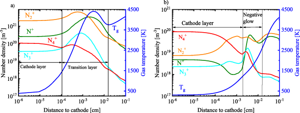
Figure 3. Axial profile of the various positive ion densities and the gas temperature in the near cathode region, for (a) the arc and (b) glow regime, at the symmetry axis (r = 0), at I = 80 mA and  .
.
Download figure:
Standard image High-resolution imageAs shown in figure 2, the electron density in the vicinity of the cathode is significantly larger in the arc than in the glow regime. There are enough electrons to create a conductive connection between the positive column and the electrodes, and hence the electric potential drop across the non-quasineutral layer in the arc regime is rather small (ca. 15 V, see figure 4; inset). The electron density in the glow regime is significantly lower, and thus, the electric field has to be much higher, for the plasma to sustain the current in this area, i.e. to accelerate the ions, which provide the same total current. This results in a very steep and very large voltage drop across the non-quasineutral layer, of 300 V (see figure 4). However, even though the mechanism of electron emission differs for the arc and glow regimes, we can see in figure 4 that the electric potential across the positive column sustains a linear dependence beyond the near-cathode region. In addition to this, the differences in the electric potential (and thus in electric field) in the positive column are small.
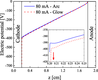
Figure 4. Axial profile of the electric potential across the discharge, for the arc and the glow case at r = 0, for I = 80 mA and  . The radius of the cathode and anode is 0.2 cm (placed at z = 0 and 2 cm, respectively).
Download figure:
Standard image High-resolution imageHere we should stress that the additional voltage at the cathode layer in the glow discharge means additional deposited power, which in this case is significant and in the same order as the rest of the discharge, i.e. ca. 24 W for 80 mA current, while the total power is 56 W. Due to the significant ion current near the cathode in the glow regime, the gas is additionally heated by the ions. Despite that, our calculations suggest that the gas temperature in the cathode fall of the glow discharge is only slightly elevated (see figure 3(b)), which is due to the intense cooling from the cathode, assumed to be at 300 K in our configuration. The gas cooling is effective due to the large surface area of the cathode region in the glow discharge and the small distance to the cathode surface. If the cathode is not cooled, the power deposited there could be sufficient for considerable gas and cathode heating and transition to an arc.
Figure 5 illustrates the 2D electron density profiles in the arc and glow regime for different currents. The cathode region looks clearly different in both regimes, for all currents investigated, i.e. it is characterized by a very high electron density, but confined in a very small region in the arc regime, while the electron density profile is quite wide with much lower values in the glow regime. Moreover, increasing the discharge current leads to qualitatively different behavior in the glow and the arc in the near-cathode region. In the glow regime, the cathode region is sustained by secondary electron emission initiated by the ion flux normal to the cathode surface. Because of this, increasing the current does not lead to more electron emission, but the current density is preserved and the cathode region enlarges radially. This effect is clearly observed in figure 5. The area of the cathode region determined from the current density increases from 0.55 × 10⁻² cm2 to 1.2 × 10⁻² cm2 and is directly proportional to the current, following the well-known fact that the current density at the cathode surface in normal glow discharges remains constant. In the arc regime, increasing the current results in even stronger field-enhanced thermionic emission. In contrast to the glow regime, the current density in the arc cathode region increases upon increasing current. The area of the arc cathode region determined from the current density remains approximately constant as a function of the current, at a value as small as 7.07 × 10⁻⁶ cm2, which corresponds to a radius of 1.5 ×10⁻³ cm. As mentioned above, this results in electron densities that are almost two orders of magnitude higher (see figure 5).

Figure 5. 2D profiles of the electron density at three different currents, for (a) the glow and (b) the arc regime, for a gas velocity  .
.
Download figure:
Standard image High-resolution imageThe significantly higher electron densities in the arc compared to the glow give rise to an increase in the vibrational temperature near the electrode. The axial profile of the vibrational temperature for 80 mA and  in the near cathode region is presented in figure 6. Within the glow, the gas temperature and vibrational temperature are nearly in equilibrium, because the electron density in the negative glow is nearly the same as in the positive column. This results in a smooth transition between the near cathode region and the positive column, leading to V-T equilibrium in the whole region. In contrast, in the arc spot, the electron density experiences a maximum (see figure 2(a)) and a sharp decline towards the positive column. Within the high electron density region, electron impact vibrational excitation (R2) deposits a significant amount of energy into the vibrational degrees of freedom, which do not have enough time to relax to the translational degrees of freedom. As a result, a maximum of the vibrational temperature is observed in the high electron density region.

Figure 6. Axial profile of the vibrational temperature for 80 mA and  in the near-cathode region.
Download figure:
Standard image High-resolution image3.2. Positive column
The key difference between the glow and the arc cathode region identified in the previous subsection is the significantly higher electron density in the arc regime at the discharge axis. This effect enhances the vibrational heating, leading to vibrational temperature much higher in the arc spot than in the glow, as shown in figure 6 above. In figure 7, the axial and radial dependence of the gas temperature, at the three different currents for both the glow and arc regime are presented. Within the positive column, the vibrational and gas temperature are in near equilibrium with each other; thus, the vibrational temperature is not shown in figure 7. The contracted nature of the plasma within the investigated current range results in high gas temperatures ( ) and negligible differences between the arc and glow discharge. In the axial direction, there is no strong gradient of gas temperature, resulting in a nearly constant axial distribution. The only differences observed between the glow and the arc are in the near-cathode region, where the arc exhibits an increase in gas temperature with rising vibrational temperature, as shown in figure 7(a). This leads to strong V-T nonequilibrium in the arc spot.

Figure 7. Gas temperature at three different currents, for both glow and arc regime, in (a) the axial direction (at r = 0, where rcathode and ranode = 0.2 cm, placed at z = 0 and 2 cm) and (b) the radial direction (at z = 1 cm), for  .
.
Download figure:
Standard image High-resolution imageThe radial gas temperature distribution at the three different currents (at z = 1 cm) is presented in figure 7(b). Upon increasing the current from 80 mA to 160 mA, the radius of the region with elevated gas temperature increases by 12.5% (from 0.24 cm to 0.27 cm), while the cross section increases by 27% (from 0.18 cm2 to 0.23 cm2).
The heating and cooling rates in the positive column for 80 mA and z = 1 cm are presented for the arc regime in figure 8. Due to similarities between the glow and arc column, only the result for the arc is shown. The heat conductivity (black curve) transports the energy radially from the middle of the column towards the side, until the convective heat transfer (red curve) stops the expansion. As a function of the current there is an increase in the gas temperature which can be seen in figure 7. The maximum gas temperature increases by 433 K, from 4483 K to 4916 K. The radial distribution of the temperature is then determined by the balance between the heat conductivity and the convective heat losses. Our analysis shows that the radial conductive component has the largest contribution to the loss mechanisms in the plasma column and the dominant heating process is V-T relaxation.
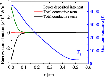
Figure 8. Heat balance in the positive column for 80 mA, arc regime, z = 1 cm and  = 1 m s−1.
Download figure:
Standard image High-resolution imageAs indicated in [13], this effect insulates the plasma from the wall, acting as a virtual cold wall. It is then logical that at a constant gas flow velocity, the positive column expands upon increasing current. The expansion of the positive column can also be seen in the radial electron density profile. The radial dependence of the electron density at three different currents, for the glow and the arc regime, at z = 1 cm and  , is presented in figure 9. Similar to figure 7, because of the contracted nature of the plasma, no differences are observed in the electron density between the glow and arc for all currents. Upon rising current from 80 to 160 mA, the electron density in the positive column experiences a small increase, from
  to
to  .
.
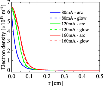
Figure 9. Radial dependence of the electron density at three different currents, for the glow and the arc regime, at z = 1 cm,  .
.
Download figure:
Standard image High-resolution imageGenerally speaking, our results show that in the positive column and the anode region, the differences in all quantities between the arc and the glow regime amount to negligible values. This effect is highlighted in figure 10, where 2D distributions of the electron density of the arc and glow case are compared to each other. Although the glow cathode region covers a significantly larger area than the arc cathode region, this does not translate to a larger area of the positive column. It is important to note that these results are not universal: they depend strongly on the chemistry and probably on the BCs and the cathode properties.

Figure 10. 2D electron density profile, at three different currents, for the arc (a) and glow (b) regime, at  .
.
Download figure:
Standard image High-resolution imageUpon increasing the current from 80 to 160 mA, the radius of the current density profile increases by 64% (from 3.8 × 10⁻² cm to 6.3 × 10⁻² cm), while the cross section rises by 167% (from 4.5 × 10⁻³ cm2 to 1.2 × 10⁻² cm2). The electron density balance was determined by analyzing equation (1). In figure 11, the total rates of production and destruction, as well as the rate of flux losses and the rate of gas convection losses, determining the electron density balance, are presented for the arc regime at 80 mA and z = 1 cm. As previously stated, due to the negligible differences in the glow and arc column, only the result for the arc is shown. The electron density balance is determined to be local and the diffusive, migrative and gas convective fluxes have a negligible contribution (see figure 11). The absolute value of the loss terms was taken in order to make the comparison between the dominant terms.

Figure 11. Production and destruction rates determining the electron density profile, for the arc regime, at I = 80 mA,  = 1 m s−1, and z = 1 cm. The glow regime has a similar radial profile, thus only the result for the arc is presented here.
Download figure:
Standard image High-resolution imageOur reaction analysis revealed that the dominant mechanism of electron production, for both arc and glow regime, is Penning and associative ionization (R28, R29, R30—table A3)


which is balanced by dissociative recombination (R32—table A4). The electronically excited  and
and  are produced primarily from quenching of the electronically excited
  and
and  states. Further analysis of the production and loss processes for the positive ions and excited states revealed that they are also locally balanced. The radial distribution of the various ion densities for the same conditions is presented in figure 12. It is clear that the dominant positive ion is N2
+ throughout most of the positive column. Near the edges of the current conductive region, where the gas temperature is lower, N3
+ becomes the dominant ion. This is attributed to the charge exchange reaction (R19—table A2). The density profile of the atomic ions N+ closely follows that of N2
+. Upon increasing current, the density of N+ approaches the density of N2
+, as also found in [18].
states. Further analysis of the production and loss processes for the positive ions and excited states revealed that they are also locally balanced. The radial distribution of the various ion densities for the same conditions is presented in figure 12. It is clear that the dominant positive ion is N2
+ throughout most of the positive column. Near the edges of the current conductive region, where the gas temperature is lower, N3
+ becomes the dominant ion. This is attributed to the charge exchange reaction (R19—table A2). The density profile of the atomic ions N+ closely follows that of N2
+. Upon increasing current, the density of N+ approaches the density of N2
+, as also found in [18].

Figure 12. Radial distribution of the various ion densities, as well as the electron density, for z = 1 cm, I = 80 mA,  = 1 m s−1, in the arc regime. Due to similarities between the glow and arc column, only the result for the arc is shown here.
Download figure:
Standard image High-resolution image3.3. Effect of the gas flow rate
In section 3.2 we demonstrated that the cathode region, and hence the electron emission mechanism, has no significant effect on the positive column. To investigate the effect of the gas flow rate on the discharge, we chose a single current condition (80 mA) and a single electron emission mechanism, i.e. thermionic field emission, hence reflecting the arc regime. We varied the inlet flow velocities as 1, 2 and 4 m s−1. The 2D velocity distributions are shown in figure 13.
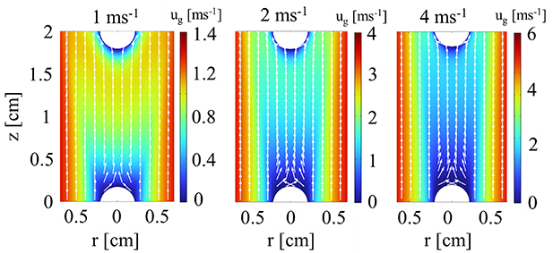
Figure 13. 2D distribution of the gas velocity magnitude, at three different inlet flow velocities, for I = 80 mA, in the arc regime. The white arrows show the velocity direction.
Download figure:
Standard image High-resolution imageWe can see that the cathode is effectively shielded by the high velocity region of the flow. A velocity gradient is present in both the axial and radial direction. As the flow velocity rises to 4 m s−1, a small recirculation zone appears above the cathode surface. The velocity in the recirculation zone is rather low and has no significant effect on the arc properties near the cathode.
In figure 14 the electron density and gas temperature profiles at the three different gas flow velocities are presented. In section 3.2 we already demonstrated, in agreement with [13], that the gas flow effectively insulates the arc from the walls through convective heat transfer in the axial direction. The increased axial cooling upon higher gas flow rate leads to further contraction of the area of the elevated gas temperature. The radius reduces by 37.5% (from 0.22 to 0.16 cm) between 1 and 4 m s−1 (see figure 14(b)), and the cross section area reduces by 87.5% (from 0.15 to 0.08 cm2). The arc radius defined from the current density profile changes from 3.8 × 10⁻² cm to 3.3 × 10⁻² cm, corresponding to a 15% decrease, and the cross section area drops by 32% (from 4.5 × 10⁻³ to 3.4 × 10⁻³ cm2). The radial temperature gradient also becomes significantly steeper upon higher gas flow velocity, which further enhances the cooling of the arc due to heat conduction and results in slightly lower temperatures in the center of the positive column. The radial profiles of gas temperature and electron density at three different gas flow velocities, for z = 1 cm, are shown in figure 15. It is interesting to see that the increase in the gas flow velocity does not influence the core of the positive column. The effects of the gas flow are primarily on the periphery of the plasma indicating the electrodes are shielding the column from the gas flow. This leads to a reduction in the radial size of the positive column without significantly affecting the core. A constant V-T nonequilibrium of ∼600 K is observed in the middle of the positive column where the electron density has it highest values (figure 15(a)). The electron density also does not experience a significant change in its maximum value as function of the gas flow (figure 15(b)).
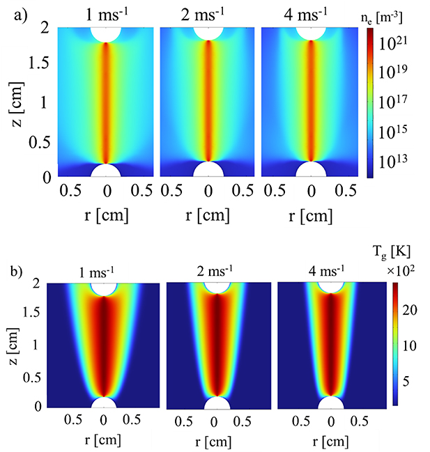
Figure 14. 2D profiles of (a) electron density and (b) gas temperature, at three different inlet flow velocities, for I = 80 mA in the arc regime.
Download figure:
Standard image High-resolution image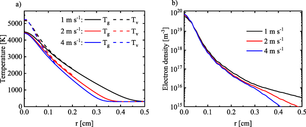
Figure 15. Radial distribution for a) the gas and vibrational temperature and b) the electron density, at three different gas flow velocities, for z = 1 cm.
Download figure:
Standard image High-resolution imageThe dominant ion remains N2 + with an increasing population of N+ upon higher flow velocities. Naturally, as the plasma is cooled down, a higher voltage is required to sustain the discharge because of the lower gas temperature of the positive column. Because the electrodes are protecting the plasma main conductive channel increasing the velocity does not lead to significant increase in the burning voltage 405 V for 1 m s−1–412 V for 4 m s−1.
Figure 16 shows the axial profile at r = 0 for the radius of the arc defined from the current density j and the gas temperature Tg. The strong coupling between the gas temperature and the electron density is observed as a function of the axial position. Following the discussion in the previous section, the radius of the region with elevated temperature is defined by the balance between the convective and conductive components, meaning that there is a strong connection between the gas velocity and the gas temperature. The electron density balance was determined to be local, indicating that the radius of the current density profile depends strongly on the gas temperature profile and indirectly on the gas velocity distribution. The gas entering the domain from the cathode towards the anode is at 300 K and gradually heats up along the axial direction. The axial transport of heated gas leads to a less steep temperature gradient in the radial direction as function of the axial position, which in turn results in expansion of the arc. This effect is highlighted in figure 16 (b) where the gas temperature radius increases as a function of the axial position for any flow rate together with the current density profile (figure 16(a)).

Figure 16. Axial profile at r = 0 of the arc radius defined from the current density profile (a) and from the gas temperature profile (b) for I = 80 mA.
Download figure:
Standard image High-resolution image4. Conclusions
We developed a fully self-consistent model of a nitrogen plasma at atmospheric pressure, including the cold cathode emission processes, which allows us to model the cathode region next to the positive column. Specifically, we compare thermionic-field emission with secondary electron emission in order to determine the influence of the cathode region on the positive column, for both arc and glow regime. Hence, our model investigates the possibility of instabilities arising from the cathode emission phenomena sustaining arc and glow discharges. The results show that for a constant gas flow velocity of 1 m s−1 and electric currents of 80, 120, and 160 mA, the different electron emission mechanisms greatly affect the size and temperature of the cathode region, which is hot and very constricted for the arc regime, and at lower temperature and more spread out (especially upon higher currents) for the glow regime. However, this different cathode region behavior does not significantly influence the positive column at atmospheric pressure. Our model also reveals that the electron density balance is local and the electron migration and diffusion are negligible under the investigated conditions. Furthermore, the contraction of the positive column and its properties are mainly determined by the balance between the conductive and convective heat transport. Finally, our model predicts that increasing the gas flow velocity does not significantly influence the peak gas temperature, and the resulting contraction weakly influences the electron density.
Our calculations inspire optimism that it is possible to create extended gas-discharge systems with a large area, sectioned cathode that can generate plasma in large volumes, regardless of the mode of the cathode layer on the cathode sections.
Acknowledgments
This research is financially supported by the European Union's Horizon 2020 research and innovation programme under Grant Agreement No. 965546.
Data availability statement
All data that support the findings of this study are included within the article (and any supplementary files).
Appendix A: Chemical reactions included in the model
Table A1. Electron impact reactions.
| Electron impact processes | Rate coefficient a , b (m3 s−1) | References | |
|---|---|---|---|
| R1 |
|

| [38, 39] |
| R2 |

|

| [38, 39] |
| R3 |
|

| [38, 39] |
| R4 |
|

| [38, 39] |
| R5 |
|

| [38, 39] |
| R6 |
|

| [38, 39] |
| R7 |
|

| [38, 39] |
| R8 |

|

| [38, 39] |
| R9 |

|

| [40, 41] |
| R10 |
|

| [40, 41] |
| R11 |
|

| [40, 41] |
| R12 |
|

| [40, 41] |
a
The rate coefficient of the reverse process is calculated by the principle of detailed balance.
b
The rate coefficient is calculated after integrating the cross section  by a electron energy distribution function calculated using BOLSIG+[39].
Table A2. Ion conversion reactions.
| Ion conversion | Rate coefficient a (m3 s−1) b | References | |
|---|---|---|---|
| R13 |
|
| [18] |
| R14 |
|

| [18] |
| R15 b |
|
| [18] |
| R16 b |
|
| [18] |
| R17 |
|
| [18] |
| R18 |
|
| [18] |
| R19 |
|

| [42] |
| R20 |

|
| [13] |
| R21 |
|
| [18] |
| R22 |
|
| [18] |
| R23 |
|

| [42] |
a In the expressions for the reaction coefficients, Tg is in K. b The units of the rate coefficients for these three-body reactions are m6s−1.
Table A3. Associative ionization and Penning ionization reactions.
| Associative ionization | Rate coefficient a (m3 s−1) | References | |
|---|---|---|---|
| R24 |
|
![${k_{24}} = 1.92 \times {10^{ - 21}}{T_{\text{g}}}^{0.98}{\left[ {1 - \exp \left( { - 3129/{T_{\text{g}}}} \right)} \right]^{ - 1}}$](https://content.cld.iop.org/journals/0963-0252/32/5/054002/revision2/psstacc96cieqn178.gif)
| [18] |
| R25 |
|
![${k_{25}} = 3.2 \times {10^{ - 21}}{T_{\text{g}}}^{0.98}[1 - {\text{exp}}{\left( { - 3129/{T_{\text{g}}}} \right]^{ - 1}}$](https://content.cld.iop.org/journals/0963-0252/32/5/054002/revision2/psstacc96cieqn180.gif)
| [18] |
| R26 |
|
| [18] |
| R27 |

|
| [18] |
| R28 |

|
| [18] |
| Penning ionization | |||
| R29 |

|
| [18] |
| R30 |

|
| [18] |
a In the expressions for the reaction coefficients, Tg is in [K].
Table A4. Electron–ion recombination reactions.
| Electron-ion recombination | Rate coefficient b (m3 s−1) | References | |
|---|---|---|---|
| R31 |
|

| [18] |
| R32 |
|

| [18] |
| R33 |
|

| [18] |
| R34 a |
|
| [13] |
| R35 |

|
| [13] |
| R36 a |

|

| [13] |
| R37 a |
|

| [18] |
| R38 a |
|
| [18] |
| R39 |
|

| [18] |
| R40 |
|

| [18] |
a The units of the rate coefficients of these three-body reactions are m6s−1. b In the expressions for the reaction coefficients, Te is in K.
Table A5. Thermal dissociation and three-body recombination reactions.
| Thermal dissociation and three-body recombination | Rate coefficient a (m3 s−1) b , c | References | |
|---|---|---|---|
| R41 |

|
![${k_{41}} = 6.6 \times 5.4 \times {10^{ - 14}}\exp \left( { - 113200/{T_{\text{g}}}} \right)\left[ {1 - {\text{exp}}\left( { - 3354/{T_{\text{g}}}} \right)} \right]$](https://content.cld.iop.org/journals/0963-0252/32/5/054002/revision2/psstacc96cieqn212.gif)
| [43] |
| R42 |

|

| [18] |
| R43 b |

|
| [43] |
| R44 b |

|

| [43] |
| Reactions involving electronically excited molecules and atoms | |||
| R45 |

|
| [13] |
| R46 |

|
| [13] |
| R47 |

|

| [13] |
| R48 |

|
| [13] |
| R49 |

|
| [13] |
| R50 |

|
| [43] |
| R51 |

|
| [18] |
| R52 |
|
| [18] |
| R53 |
|
| [18] |
| R54 |

|
| [18] |
| R55 |

|
| [18] |
| R56 |

|
| [18] |
| R57 |

|
| [18] |
| R58 c |
|
| [18] |
| R59 c |
|
| [13] |
| R60 b |
|

| [18] |
| R61 |
|
| [18] |
| R62 |
|
| [43] |
| R63 |
|
| [18] |
| R64 |
|
| [18] |
a In the expressions for the reaction coefficients, Tg is in K. b The units of the rate coefficients of these three-body reactions are m6 s−1. c The units of the rate coefficients of these radiative decay reactions are s−1.


Appendix B: Comparison with experiments
Our model was calculated for the experimental conditions in [18] and the results of the electron density as a function of the current are presented in figure B1. Our calculated electron density is about one order of magnitude larger than the value of [18], and is more or less constant upon increasing current, while the data of [18] rise with current. Even though we have the same kinetic mechanisms in [18] our model is not able to reproduce the results. We attribute this to the complicated gas flow behavior of the experiment, which is not explained in detail. Our modelling approach requires information of the full geometry in order for us to calculate the flow field. We performed additional comparison with the experiments in [13] presented in figure B2.

Figure B1. Comparison of the electron density (at z = 1 cm) from our model, with the results of [18].
Download figure:
Standard image High-resolution image
Figure B2. Comparison of the vibrational temperature Tv and gas temperature Tg (at z = 1 cm) for our model and the experimental results in [13] for different currents.
Download figure:
Standard image High-resolution image
There is good agreement between the experiment and our model for the values of the gas temperature as a function of the current. The experimental vibrational temperature shows a decreasing trend as a function of the current and approaches (near) equilibrium with the gas temperature, while our model shows an increase in vibrational temperature and strong deviation from equilibrium. The discrepancy between our model and these experiments might be because some kinetic pathway is still missing, or because we do not have all the information on the full geometry of these experiments, which would be needed for an accurate description, due to the strong coupling between gas flow and plasma behavior in our model. However, we believe our present model can already qualitatively describe the differences between arc and glow regime, and the effect on the plasma column, which was the purpose of our work.