

Abstract
Urbanization, a major driver of global change, profoundly impacts our physical and social world, for example, altering not just water and carbon cycling, biodiversity, and climate, but also demography, public health, and economy. Understanding these consequences for better scientific insights and effective decision-making unarguably requires accurate information on urban extent and its spatial distributions. We developed a method to map the urban extent from the defense meteorological satellite program/operational linescan system nighttime stable-light data at the global level and created a new global 1 km urban extent map for the year 2000. Our map shows that globally, urban is about 0.5% of total land area but ranges widely at the regional level, from 0.1% in Oceania to 2.3% in Europe. At the country level, urbanized land varies from about 0.01 to 10%, but is lower than 1% for most (70%) countries. Urbanization follows land mass distribution, as anticipated, with the highest concentration between 30° N and 45° N latitude and the largest longitudinal peak around 80° W. Based on a sensitivity analysis and comparison with other global urban area products, we found that our global product of urban areas provides a reliable estimate of global urban areas and offers the potential for producing a time-series of urban area maps for temporal dynamics analyses.
Export citation and abstract BibTeX RIS

Content from this work may be used under the terms of the Creative Commons Attribution 3.0 licence. Any further distribution of this work must maintain attribution to the author(s) and the title of the work, journal citation and DOI.
1. Introduction
The transformation of terrestrial environments by urbanization has been accelerating over the past 30 years (Chen et al 2014), and is likely to continue due to population growth and migration. Accompanying this process is a range of environmental consequences, with important socio-economic implications (Poumanyvong and Kaneko 2010). Urban expansion into vegetated lands compromises ecosystem services by reducing photosynthetic production, altering carbon flux, and threatening biodiversity (Imhoff et al 2004, Foley et al 2005, Parshall et al 2010, Zhou et al 2010, Martínez-Zarzoso and Maruotti 2011, Zhou et al 2013, Aronson et al 2014). Biophysical changes associated with impervious surfaces modify energy and water partitioning and thus influence local and regional surface climates (Hansen et al 2001, Kalnay and Cai 2003). Built environments not only trap heat and influence local precipitation patterns but also degrade air quality by changing atmospheric chemistry and aerosol composition (Stone 2008). Urban growth also alters social demography and economic conditions, especially in developing countries, and change energy and resource demands. These alterations in environmental and social conditions interact to influence public well-being and health (Gong et al 2012, Van de Poel et al 2012). Understanding these interactions is essential to tackle ongoing global changes. The level of understanding hinges greatly on the availability of accurate and consistent information on the distribution and extent of urban areas.
Although census and survey data have been a traditional source for creating urban maps, spatially-explicit urban mapping has been increasingly attempted using remotely sensed observations, especially over large geographical regions (Zhou and Wang 2007, Zhou and Wang 2008, Schneider et al 2009, Zhang and Seto 2011). During the last few decades, there has been a proliferation of remote sensing-based urban maps for a wide range of scales. In particular, satellite multispectral images, routinely available from Landsat and other satellites, provide valuable spectral data for mapping cities and impervious surfaces worldwide, and such products offer critical information to examine human-environment interactions for scientific studies and assessments of social and environmental consequences of urbanization (Homer et al 2007). Recent technological advances in remote sensing, such as high-resolution imaging and airborne LiDAR, make it possible to derive detailed 3D urban structures at the individual building level (Zhang et al 2006). At the other end of the spectrum, enhanced computing power together with increased availability of remote sensing data permit generating reliable urban maps for the entire globe, consistently (Schneider et al 2009).
Existing global urban maps derived from remote sensing, offer spatially-consistent sources of information valuable for global environmental studies, although these products have their own limitations (Stone 2008, Parshall et al 2010, Zhou et al 2010). One product in wide use is the global urban map created from the moderate resolution imaging spectroradiometer (MODIS) data circa 2001–2002 by the MODIS land-cover team (Schneider et al 2009, Schneider et al 2010). This map represents a major advance in mapping urban areas globally, attributable particularly to the high quality of spectral measurements; it also overcomes some deficiencies, such as inconsistencies in urban definition, scale, and data quality, in earlier global maps derived from other sources (Schneider et al 2010). Despite these recent advances, challenges and difficulties still exist in generating consistent and accurate global urban area maps and derived products. For instance, it is challenging or labor-intensive to build temporally resolved maps/products, therefore, limiting application for dynamic analysis.
The defense meteorological satellite program/operational linescan system (DMSP/OLS) nighttime stable light (NTL) data can provide a systematically collected global dataset, and has a number of unique features that meet the needs of widescale, frequently repeated surveys of urban growth (Henderson et al 2003, Elvidge et al 2009). Most importantly, the DMSP/OLS NTL data have a reasonable temporal coverage at the global level from 1992 to present. The DMSP/OLS NTL data offer potential for regional and even global urban maps and their application in studies of human activities, such as population density, economic activity, energy use, and CO2 emissions (Imhoff et al 1997, Doll et al 2000, Elvidge et al 2007a, Zhang and Seto 2011, He et al 2014, Naizhuo et al 2015).
Although the use of DMSP/OLS NTL data has been demonstrated in previous studies of urban area mapping, it still has several shortcomings, such as limited dynamic range, signal saturation in urban centers resulting from standard operation at the high gain setting, lack of a well-characterized point spread function (intensity profile from point source), and lack of a well-characterized field of view (a measure of the spatial resolution) (Elvidge et al 2010). It has been documented that the DMSP/OLS NTL data tend to exaggerate the size of urban areas compared to the Landsat analysis, because OLS-derived light features are substantially larger than the lighting sources on the ground (Imhoff et al 1997, Henderson et al 2003, Elvidge et al 2009).
Threshold techniques have been developed to address these challenges of urban mapping from NTL data and showed potential in generating reasonable urban products at the regional and national scales (Imhoff et al 1997, Henderson et al 2003, Amaral et al 2005, Kasimu et al 2009). However, under- and over- estimation of urban area extent has been a major issue when using a single threshold in regional or national urban mapping. Zhou et al (2014) developed a cluster-based method to estimate optimal thresholds for mapping urban extent using DMSP/OLS NTL for the US and China. Based on this method, the optimal threshold for each potential urban cluster is estimated according to urban cluster size and the overall nightlight magnitude in the cluster, resulting in specific thresholds for each urban cluster, thus reducing significantly over- and under- estimation in general threshold methods.
This study aims to build a globally consistent and temporally updateable urban extent map from the DMSP/OLS NTL data. The global map is created by extending the cluster-based method with a new parameterization scheme. This new global map is evaluated by comparing it to several existing global products and also by performing sensitivity analyses.
2. Data and method
2.1. Data
The major data used in this study include the DMSP/OLS NTL, high spatial resolution land cover, water mask, and gas flare mask. The DMSP/OLS NTL measures lights on the Earth surface from cities and settlements with persistent lighting, and other sources such as gas flares, fires, and illuminated marine vessels (Zhang et al 2013). The data were recorded as digital number (DN) from 0 to 63 with a 1 km spatial resolution, spanning −180° to +180° in longitude and −65° to +75° in latitude. Annual cloud-free composites were built using the highest-quality data based on a number of constraints (Elvidge et al 2009). The NTL data in the year 2000 were chosen to build the global product of urban areas for validation and comparison with other similar products. The water mask was derived from MODIS 250 m land–water mask (MOD44W), and gas flare data were obtained from the NOAA national geographic data center (Elvidge et al 2009).
High-resolution land cover data for the US in 2006 and China in 2005 were obtained from US Geological Survey National Land Cover Dataset (NLCD) and Resources and Environment Data Center of the Chinese Academy of Science, respectively, both with an original spatial resolution of 30 m (Homer et al 2004, Liu et al 2010). Land cover types mainly include open water, urban, evergreen forest, deciduous forest, shrub, grassland, cropland and wetland. The land-cover data for China were built through visual interpretation of Landsat TM images and aggregated to a 1 km scale map of each land cover type (Liu et al 2010). The US land-cover data layer was also aggregated from 30 m to 1 km spatial resolution, resulting in an urban percentage map.
A unified definition of 'urban' has not been reached, and thus the estimates of global urban land vary widely with different definitions in previous studies (Liu et al 2014). In this study, similar to Zhou et al (2014), we define urban land as those 1 km pixels with urban percentages larger than 20%, consistent with the developed areas in the US NLCD dataset (Fry et al 2011).
2.2. Method
2.2.1. Cluster-based method
The threshold techniques were developed to delineate urban extent based on the DMSP/OLS NTL observation to account for the bias of light features in NTL being substantially larger than the lighting sources on the ground. The threshold is defined as the DMSP/OLS DN value above which the pixel is classified as urban area. Moreover, urban pixels tend to group together as clusters. As such, our cluster-based method generally follows this logic by segmenting the NTL into clusters and delineates urban extent in each cluster based on the NTL DN values and a cluster-specific threshold.
Our method for mapping global urban area is an extension of the cluster-based method originally developed in Zhou et al (2014). This revised method includes five major steps: data preprocessing, urban cluster segmentation, parameterization for the logistic model, threshold estimation, and urban extent delineation (figure 1). First, as a pre-processing step, water and gas flare pixels are excluded from the NTL data. Second, using a marker-controlled watershed segmentation algorithm (Zhou et al 2014), the processed NTL data were segmented into potential urban clusters, each consisting of groups of similar and spatially continuous pixels. Not all pixels in each potential cluster are urban. More details about segmentation can be found in Zhou et al (2014).
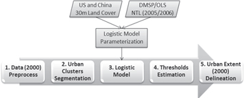
Figure 1. The cluster-based urban mapping method.
Download figure:
Standard image High-resolution imageThird, an optimal threshold for each cluster is then estimated to delineate the actual urban area from the NTL data in each potential urban cluster. To estimate the optimal threshold, we developed a logistic model with two parameters a/b and β', as formulated in equations (1) and (2). This model ingests cluster-level NTL information and gives an estimate of optimal threshold for delineating urban extent in each cluster. Building on the work by Zhou et al (2014), we developed a parameterization method to estimate a/b and β' and calculated these two parameters for each country (see next section 2.2.2). Here our parameterization method was developed from the NTL data in years 2006 and 2005 for the US and China, respectively, in order to be temporally consistent with the available high spatial resolution land cover dataset. The optimal threshold is calculated as follows

where x' is the index for estimating the optimal threshold based on combined effects of both mean lighting magnitude and cluster size, S is the cluster size, NTLmean is the mean NTL DN in each cluster, and a/b is the parameter for the relative contribution of each of two effects. NTLthld is the optimal threshold to delineate the urban area in the potential cluster, and x'mean is the mean value of x'. NTLmin and NTLmax are minimum and maximum NTL DN in the study area, and β' is the parameter in the logistic model.
Fourth, we estimated the optimal threshold value for each cluster identified from the year 2000 global NTL data at the global level using the logistic model and the derived parameters in step 3. Finally, we mapped the urban extent according to the estimated optimal threshold in each cluster. We chose the NTL data in the year 2000 to build the global urban area product because of the availability of other datasets such as MODIS urban product close to this time period for validation and inter-comparison.
2.2.2. Parameterization of the logistic model
In this study, we developed a parameterization method to estimate the key parameters (a/b and β') in the logistic model using the NTL data only. As reported by Zhou et al (2014), the parameters of a/b and β' in the logistic model show slight difference in the US and China at the country level, although the optimal thresholds are not highly sensitive to these parameters. We calculated these two parameters at the regional level by dividing the US into nine Census regions, and dividing China into three economic regions (figure 2). The optimal thresholds derived from high spatial resolution reference data for the US in 2006 and for China in 2005 were used to estimate these two parameters in the logistic model in each region according to the method by Zhou et al (2014). We performed this analysis at the regional level for several reasons. First, we can collect a number of samples to evaluate the variations of these two parameters. Second, because of differences in factors such as socioeconomic development and geography, these regions can cover a range of urbanization. Third, it can reduce the possibility of separation of potential urban clusters across different regions. The possibility of shared clusters across boundaries is high at finer spatial units, such as province or state.

Figure 2. Map of regions for parameterization and sensitivity analysis.
Download figure:
Standard image High-resolution imageIn order to extend the logistic model in other regions without high spatial resolution data, we analyzed the two parameters (a/b and β') in the logistic model for all regions in the US and China. We found that the parameter a/b has a narrow distribution around 0.23 with a standard deviation of 0.01 (figure 3(a)), and that the parameter β' is highly correlated to regional nightlight mean magnitude for each region (figure 3(b)).

Figure 3. The frequency of a/b for 12 regions (a) and the relationship between β' and regional nightlight mean magnitude (b). a/b and β' are the parameters in the logistic model. The numbers correspond to those in figure 2.
Download figure:
Standard image High-resolution imageBased on this analysis, we took the mean value of 0.23 for a/b, for the logistic model in each country. The parameter β' for each country was derived from the regression equation between this parameter and regional nightlight mean magnitude (figure 3(b)). It is worth noting that the parameterization scheme could also be applied at a sub-national level to further improve urban mapping in large countries, particularly for regional scale urban studies. Although this paper is focused on global urban mapping, we evaluated the sensitivity of the optimal thresholds to these two parameters to evaluate the reliability of this parameterization scheme (see the results and discussion section below).
3. Results and discussion
3.1. Global map of urban extent
The newly developed 1 km urban product was aggregated to 1/12° as a percentage map (figure 4) to be comparable with other previously published products. Based on this new map, overall urbanization at the global level is about 0.54%, which is close to 0.49% derived from MODIS observations (Schneider et al 2009). Urban areas show large spatial heterogeneity, globally. The global distribution of urban area as depicted in figure 4 appears realistic, and it is not surprising that Europe shows the largest urbanized fraction (2.3%) as compared with other regions, with North America next at 1.2%. The urbanized land in Asia, Latin America, and Former Soviet Union (FSU), and Oceania are 0.7%, 0.4%, 0.2%, and 0.1%, respectively. The urbanized land in Africa is less than 0.1%, the lowest among all regions.
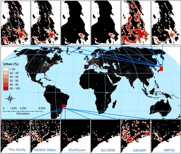
Figure 4. A global map of urban extent derived from DMSP nightlight data. The two enlarged example areas compare this new product with the five previously published global urban maps.
Download figure:
Standard image High-resolution imageAt the country level, urban land area varies from lower than 0.01% to higher than 10%. Urban land area in most countries (>70%) is less than 1%, and more than 90% of countries have urban land area of less than 5% (figure 5). In some regions such as FSU, urban land area in all of the countries within the region covers less than 1% of total land area. Urban land area in large countries such as Russia, with a large amount of areas in high latitude zones, is close to 0.1%. The countries with relatively high urban land area are mostly in Europe. Among the large countries, the US has urban land area of more than 1%.
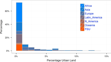
Figure 5. Distribution of countries in terms of percentage of urban land area, for different regions, globally.
Download figure:
Standard image High-resolution imageMajor urban clusters are further uncovered by the longitudinal and latitudinal distributions of both urban area and percentage (figure 6). The latitudinal zones around 30° N have the largest urban area due to contributions from China and the US, while the latitudinal zones with the highest urbanized percentage move North, around 45° N, largely due to the influence of European countries. The longitudinal distribution of urban area shows several large centers. One of the most evident ones is around 80° W, encompassing the 'Boston–New York–Washington' corridor of the US Northeast region, and this longitudinal distribution of urbanized percentage is consistent with that of total urban land area. This type of analysis is useful for developing adaptation and risk management measures for urban infrastructure, transportation, energy, and water systems when considered together with other factors such as climate variability and change, and high impact weather events.

Figure 6. Urban area distribution by longitude and latitude. Urban area and percentage are calculated in each 1/12° of longitude and latitude zone. Red is total urban area in each zone and blue is urbanized percentage of total land area in each zone.
Download figure:
Standard image High-resolution image3.2. Sensitivity analysis of logistic model parameters
Two sensitivity analyses were performed to examine the impact of the parameters of a/b and β' on the selection of the optimal thresholds (figures 7 and 8). In the first analysis, we evaluated the R2 and root mean squared error (RMSE) between the optimal thresholds derived from high resolution land cover data and our logistic model by varying the parameters (a/b and β') in a range of possible values (figure 7). The results indicate that the choice of these parameters have small impact on the R2 when a/b is lower than 0.3, and that R2 values begin to decrease when a/b is larger than 0.3, and the RMSE reaches its minimum value when a/b falls in the range of 0.2–0.25, for most regions. More important, the RMSE is as low as 4 when a/b is within a range of 0.15–0.3, for all regions. The impact of parameter β' on the R2 is also minor, and it reaches its maximum R2 value around 0.9 in most regions when β' falls in the range of 0.75–1.0. The RMSE is as low as 3 when β'is within the same range.
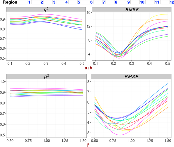
Figure 7. Sensitivity of the optimal thresholds for parameters of a/b (top) and β' (bottom). a/b and β' are the parameters in the logistic model. The region numbers correspond to those in the figure 2.
Download figure:
Standard image High-resolution image
Figure 8. Comparison between optimal thresholds derived from high-resolution land cover data and those from the logistic model using parameters of a/b (=0.23) and β' (estimated from a regression equation). The numbers on the gray strip correspond to those in the figure 2.
Download figure:
Standard image High-resolution imageThe first sensitivity analysis indicates that the sensitivity of the optimal thresholds to the two parameters (a/b and β') is low when these parameters are sufficiently close to their optimal values. Then, in the second analysis, we examined the difference between optimal thresholds from high-resolution land cover data and those using the logistic model with parameters of a/b = 0.23 and β' derived from the regression equation for each region (figure 8). The results indicate that the parameterization method in the logistic model based on a regression equation for the parameter β' together with a mean value (0.23) for the parameter a/b performs well in determining the optimal thresholds for all study regions.
3.3. Evaluation
We compared the global map of urban extent from NTL to five previously published and widely used global urban area products approximately for the same period. These include (1) MODIS 500 m urban map (2001–2002); (2) GlobCover (2005); (3) GLC2000 (2000); (4) global rural–urban mapping project (GRUMP) (1995); and (5) NOAA's impervious surface area map (IMPSA) (2000–2001), at the pixel level for two selected sites (figure 5), and regionally (figure 9). The derived urban area from MODIS data is defined as built environment including all non-vegetative and human-constructed facilities that cover greater than 50% of a given landscape unit (Schneider et al 2009). The urban area estimates in GlobCover and GLC2000 are defined as artificial surfaces and associated areas (Bartholomé and Belward 2005, Bicheron et al 2008). The urban area in GRUMP is defined as urban extents with the total population greater than 5000 persons (CIESIN 2011). The urban areas in IMPSA is based on the density of impervious surface area (Elvidge et al 2007b).

Figure 9. Urban areas (on a log scale) from six datasets, at the regional and global levels.
Download figure:
Standard image High-resolution imageFor the first site in Japan with highly urbanized land, our newly developed product shows the greatest similarity in spatial pattern and urbanization magnitude with the MODIS product. The extent of urban areas in GlobCover and GLC2000 is much smaller compared to other datasets, while the urban extent in GRUMP is the largest among the six products. The urban extent in IMPSA is similar to our estimate and the MODIS product, but its magnitude is smaller. For the second site in Brazil with medium urbanized land, the urban extent and magnitude in our data, the MODIS product, and IMPSA are similar, while the urban extent is still smaller in GlobCover and GLC2000, and larger in GRUMP compared to the other products.
Similar to the comparison at the two selected sites, total urban land area in our newly developed product is closest to the MODIS product at both global and regional levels (figure 9). Urban areas in GlobCover and GLC2000 are generally lower than all other products, and urban area in GRUMP is the highest at the global and regional levels. Urban area in IMPSA is generally lower than our estimation and those from MODIS product, except for Asia. There are several factors, such as definition of urban extent and data used, contributing to the difference between products. Different from these products, often limited by the temporal coverage of used geospatial data, the proposed method in this study provides the possibility to build temporally updateable urban area maps using the long time series of DMSP/OLS NTL data.
We evaluated our urban area product at the pixel level using the five global urban products discussed above as reference data (figure 10). A kappa coefficient of 0.41–0.60 indicates moderate agreement, and a value of 0.61–0.80 indicates substantial agreement (Viera and Garrett 2005). Based on this analysis, we find our newly developed urban area product to be in substantial agreement with the IMPSA product for most regions, globally. One reason for this high degree of agreement is that both products use the same input data, including NTL and NLCD, in mapping urban areas. As the IMPSA method requires auxiliary data such as gridded population, it needs more effort to develop a global product. The requirement for auxiliary data also limits its capability in mapping temporal urban dynamics. It would be useful in future work to examine if the methodologies developed here could be extended to also produce information on impervious surface area, given its importance for applications such as hydrology modeling.

Figure 10. Comparison of urban area between newly developed urban area map and five previously published global urban area map products.
Download figure:
Standard image High-resolution image
The agreement for North America is also high between our product and all other products except for GlobCover. For all regions, our product is in moderate agreement with MODIS product, and especially in substantial agreement for North America, South America, and Oceania. At the global level, our product is in almost substantial agreement with MODIS product. Our newly derived urban area map achieves an overall high comparability with other five products for all regions. According to the measurement of omission error, our product varies the most compared with the GRUMP product, while the omission error is the lowest compared with IMPSA product. The omission error for urban area in our product is lowest in North America, as compared with all five products. According to the measurement of commission error, our product varies the most compared with the GlobCover product, while the commission error is lowest compared with GRUMP product. The commission error for urban area in our product is lowest in Oceania region, compared with all five products.
In addition to the evaluation against other products at the global level, we chose Europe, a region not used in our model development, to assess the accuracy of the derived urban extent using the 100 m spatial resolution Corine land cover 2000 data set (Büttner et al 2004). While our global product is targeted for large-scale urban area mapping and monitoring, and it is also limited by the spatial resolution of NTL data, we believe that the resulting pixel level accuracy (overall accuracy of 87%, Kappa coeeficient of 0.55, producer accuracy of 96%, and user accuracy of 88%) for Europe is reasonably good.
4. Conclusions
We developed a global urban area map at 1 km spatial resolution based on a new cluster-based approach applied to DMSP/OLS NTL data. The comparison of our product with other five global urban area products indicates that the new product is robust and provides a reliable estimation of global urban land area. A sensitivity analysis shows that the parameterization method in the logistic model performs well in determining the optimal thresholds for delineating urban extent from DMSP/OLS NTL observations.
We found the global urban land area to be about 0.5% of total land area. Regionally, it ranges from 0.1% in Oceania to 2.3% in Europe. Nationally, urban land area varies from lower than 0.01% to higher than 10%, with urban land area being less than 1% in more than 70% countries. The latitudinal zones around 30° N have the largest urban area, with highest urbanized land area moving Northward to the 45° N region. Generally, the largest urban land area is located in 30° N to 45° N region. Longitudinally, there are several highly urbanized zones, and the highest region is around 80° W. This information is of great value for developing adaptation and risk management measures for urban infrastructure and systems, in the context of global environmental changes and their impacts on natural ecosystems, people and infrastructure.
One avenue for future research is to address the lack of globally consistent urban area product over a sufficiently long period of time. Such a time-series would be valuable for uncovering drivers of urban expansion, modeling urban growth dynamics, and predicting future urbanization. Although there are multiple historical maps, they are often static and non-continuous in capturing urban extents across time and space; additionally, these maps are often incompatible due to the use of varying urban definitions, data, or methods. These limitations highlight a pressing need to develop consistent global urban maps over time. The method developed in this study allows the use of DMSP/OLS NTL data, which has been acquired continuously since 1992, without using supporting data such as vegetation index that may be limited in temporal coverage. The simplicity of our proposed method together with the availability of long-term satellite data sets shows promise for rapidly monitoring urban areas globally and regionally.
Acknowledgments
We acknowledge the funding support from NASA ROSES LAND-COVER / LAND-USE CHANGE program (NNH11ZDA001N-LCLUC). We thank Dr Yaling Liu for a very useful internal review, and the many colleagues and organizations that shared data used in this project. The global map of urban area extent produced in this study can be requested from yuyu.zhou@pnnl.gov.