Developing Non-Negative Spatial Autoregressive Models for Better Exploring Relation Between Nighttime Light Images and Land Use Types

Abstract

Exploring the relationship between nighttime light and land use is of great significance to understanding human nighttime activities and studying socioeconomic phenomena. Models have been studied to explain the relationships, but the existing studies seldom consider the spatial autocorrelation of night light data, which leads to large regression residuals and an inaccurate regression correlation between night light and land use. In this paper, two non-negative spatial autoregressive models are proposed for the spatial lag model and spatial error model, respectively, which use a spatial adjacency matrix to calculate the spatial autocorrelation effect of light in adjacent pixels on the central pixel. The application scenarios of the two models were analyzed, and the contribution of various land use types to nighttime light in different study areas are further discussed. Experiments in Berlin, Massachusetts and Shenzhen showed that the proposed methods have better correlations with the reference data compared with the non-negative least-squares method, better reflecting the luminous situation of different land use types at night. Furthermore, the proposed model and the obtained relationship between nighttime light and land use types can be utilized for other applications of nighttime light images in the population, GDP and carbon emissions for better exploring the relationship between nighttime remote sensing brightness and socioeconomic activities.

1. Introduction

Nighttime light recorded by satellites represents what human beings use at night for production and living, which is an effective means to study the spatial distribution of human nocturnal activities [1,2]. It has been confirmed that there is a strong linear correlation between night light brightness values and various economic indicators in a region [2,3,4]. So, night light data have been widely used to simulate the spatial distribution of the population, GDP, carbon emissions and other fields [4,5,6]. However, studies have also shown that the correlation between night light and economic indicators varies from region to region [7,8,9]. For example, the nighttime light intensity (NLI) of an American town with a population of 10,000 is three times that of a German town of the same size [10]. Studying the regional differences and influencing factors in the correlation between night light and economic activities can help researchers correct the errors in estimating GDP and economic activities by using night light, improving the accuracy of GDP estimation, and reflecting the spatial distribution of GDP accurately [11,12]. In addition, only by understanding the causes and distribution pattern of night light can we more accurately explain and analyze the distribution rules of human nighttime activities [13,14], study socioeconomic problems [15,16] and prevent and control light pollution [17,18] with night light data.

From a physical point of view, land use is an important method to explain the distribution of light at night [19,20]. Different types of land uses have different circadian rhythms of human activities, and the brightness of light emitted at night is different [21]. Relationship between land use and night lights has drawn the attention of experts in the fields of atmospheric science, remote sensing, ecological protection and economics [22,23,24,25]. In the field of astronomy and atmospheric science, traditional night light detection methods use instruments for ground measurement, which requires intensive manpower [26,27]. In recent years, aerial photography for nighttime lighting sources has been used. Helga used nighttime aerial images with a resolution of 1 m to study the main sources of nighttime light in Berlin [28]. However, the method of using nighttime aerial images and ground measured data to study the cause of night light is expensive, and it is difficult to apply in areas without ground measurement as well as in comparative studies of the relationship between night light and land use type in different regions. Therefore, an efficient and widely applicable method to compare the relation between night light and land use types in different regions is desired.

The method of using satellite images to study night light simultaneously records the distribution of light brightness in a large range and reflects the time sequence of the changing light in a specific region, which is convenient and cheap [29]. However, the resolution of satellite images of night light is relatively low, and the accuracy of existing land use data is much better than that of night light data, so there are multiple mixed distributions of land use in the same pixel. In order to correlate the two datasets with different resolutions, it is necessary to decompose the contributions of various land use types to night light by appropriate models. A regression model can investigate the relationship between different independent variables and dependent variables, but the assumptions of different models are distinct. Conventional regression models cannot reflect the actual luminescence contributions of the land use types because of the existence of a negative regression coefficient. Therefore, it is necessary to introduce non-negative constraints to the regression model, which have been widely used in model optimization for reducing combinations and improving sparsity and model efficiency [30,31,32]. Li proposed a non-negative least-squares method for modeling low-resolution nighttime light data with high-resolution land use data [33]. Although this method obtained a more accurate nighttime light index of different land use types, it did not take the influence of the surrounding pixels into account when using the land use area to model the brightness of a pixel. The light emitted from the objects in the interior of a pixel may affect the brightness of the surrounding pixels through light refraction and reflection [34,35,36]. Ma furtherly found that the land use type affected the correlation between the night light data and human activity data on the pixel scale, and this was analyzed with the method of spatial autocorrelation [37]. It proved that the spatial autocorrelation effect of night light data needs to be considered when studying the relationship between night light data and other data. Therefore, when using nighttime remote sensing images to explore the NLIs of various land use types, the spatial autocorrelation effect between pixels should be eliminated [38,39], in addition to solving the land use type mixing problem.

The main goal of this research was to analyze the nighttime light component, specifically the correlation between night light and land use by non-negative spatial autoregressive models. In this model, the spatial autocorrelation effect of night light images is solved by taking the brightness of adjacent pixels into account. The two models, the non-negative spatial Lag model (NSLM) and the non-negative spatial error model (NSEM), are developed and compared with the traditional non-negative least-squares model. The results show that our method has a higher R² and lower Akaike information criterion (AIC) value with the reference data overall. It was found that NSEM is suitable for small neighborhoods of high-resolution data, and NSLM has a better effect on large neighborhoods of low-resolution data. Through this method, we can obtain a more accurate NLI value, which is of great significance for solving the following problems: (1) to better distinguish the relationship between different land use types and night light data, and reflect the source of nighttime light more accurately and (2) to find land use types closely related to human nighttime activities and expand the application field of nighttime light data in the study of human activities, such as light pollution, traffic, GDP components, and so forth.

2. Methods

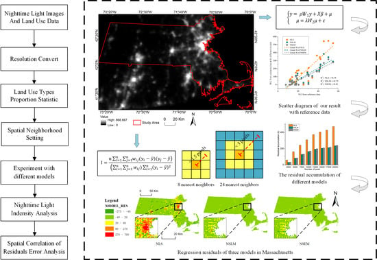
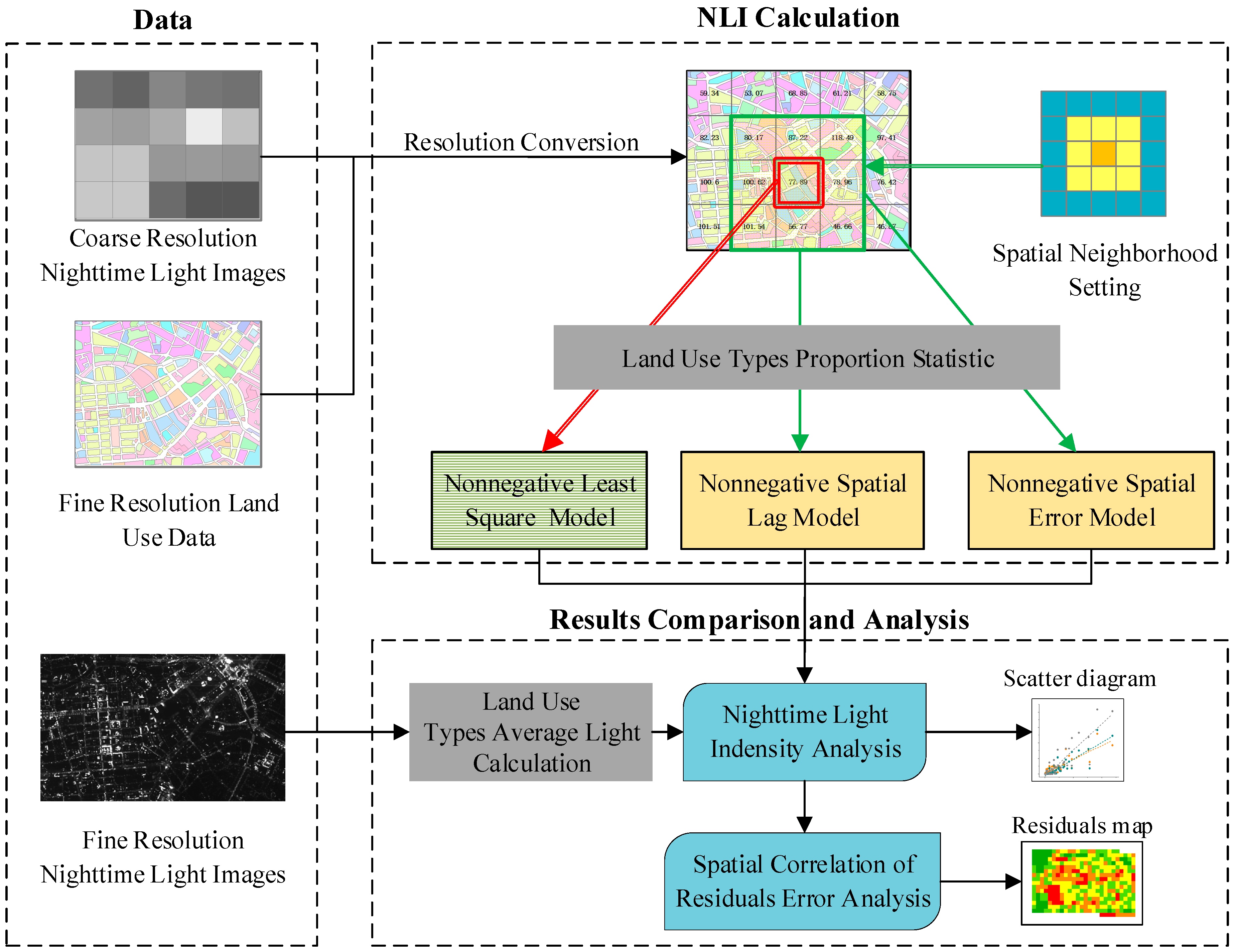
In this study, non-negative spatial autoregressive models and corresponding solving methods are developed to quantify the land use contribution to nighttime light using coarse-resolution night imagery and fine-resolution land use data. The experimental framework is shown in Figure 1, including resolution conversion, land use type proportion statistics, spatial neighborhood setting, NLI calculation by different models and results comparison and analysis.

2.1. Study Area and Data Sources

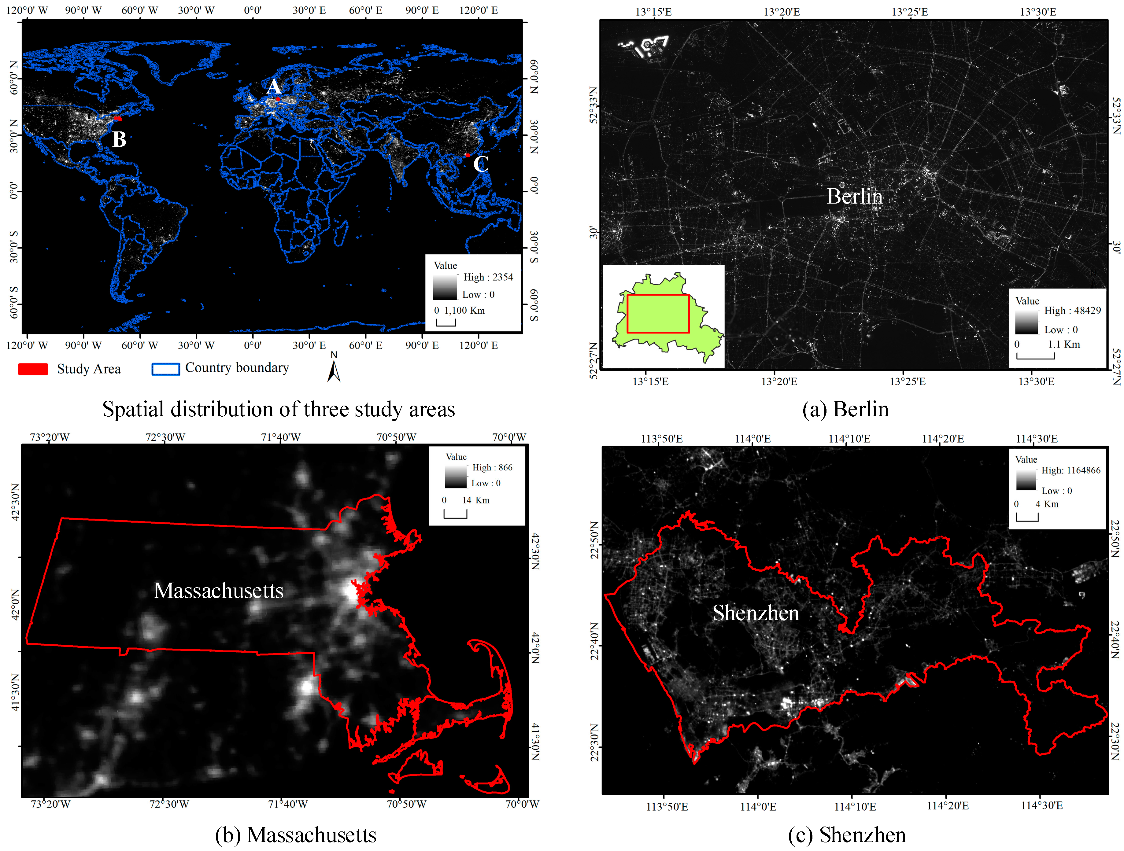
The study areas were Berlin in Germany, Massachusetts in the United States, and Shenzhen in China. Since the three areas are the mostly developed regions in these countries, there were abundant remote sensing images and statistical data available online for supporting this study. The selected data covered large time spans and diverse spatial resolutions. In addition, the three areas are located in different countries with distinct levels of economic and urban development stages. These features can help to verify the robustness and adaptability of the models in different application scenarios. The nighttime light images and the administrative boundaries of the three study areas are illustrated in Figure 2.

With a population of 3.7 million, Berlin is the largest city in, and the capital of Germany [40]. Berlin is also a city with a high level of economic development and a good ecological environment. About one-third of the area is composed by forests, parks, gardens, rivers, canals and lakes. With an area of 27,340 km² and population of 6.9 million in 2018, Massachusetts is the third most densely populated state in the U.S. [41]. As one of the original 13 states, Massachusetts has a long history of development. Over 80% of Massachusetts’ population lives in the Greater Boston metropolitan area that has great influential upon U.S. history, academia and industry. Shenzhen is the first special economic zone in China and the major city in the Pearl River Delta megalopolis. With a population of 12.5 million in 2017, Shenzhen ranked as the third largest city in China [42]. As a newly developed city after the reform and opening up, Shenzhen has become one of the most economically dynamic cities in China, and even the world.

The experimental data of the three study areas are shown in

Table 1. Experimental data of the three research areas.

Data Sources			Berlin	Massachusetts	Shenzhen
Analysis data	Land use Data	Acquisition time	2010	2005	2015
		Resolution	5 m	0.5 m	1 m
		Number of types	52	33	26
	Coarse resolution nighttime light image	Source	Annual composite product of NPP/VIIRS	DMSP/OLS images	Annual composite product of NPP/VIIRS
		Acquisition time	2012	2005	2015
		Resolution	500 m	1 km	500 m
Reference data		Source	Aerial photography	Photograph from the International Space Station	Product from LuoJia1-01
		Acquisition time	2011	2010	2018
		Resolution	1 m	30 m	170 m

. The data used for building the regression model were land use data and coarse resolution nighttime light images. Reference data were fine-resolution nighttime light images for model accuracy verification.

2.2. Data Preprocessing

2.2.1. Resolution Conversion

The raw night light images used in this paper were the average annual images of Defense Meteorological Satellite Program’s Operational Linescan System (DMSP/OLS) and Visible Infrared Imaging Radiometer Suite (VIIRS) sensor on the Suomi National Polar-orbiting Partnership (NPP) Satellite. Radiometric correction has been conducted, and the background noise of the images has been removed by data providers [33,43,44]. Since this study does not involve time series analysis, the joint correction of NLI values between yearly images is not needed. So, the projected transformation and resolution conversion were performed directly with the downloaded images.

All images of the same study areas were projected into the same geographic coordinate system. Images of Berlin, Shenzhen and Massachusetts were projected into World Geodetic System 1984(WGS84)/Universal Transverse Mercator (UTM) zone 33N, zone 49N and the State Plane (Mass Mainland) coordinate system, respectively. As the nighttime light images and land use data had different resolutions, fine-resolution land use data were converted to a coarse resolution that of the nighttime light images for further analysis.

2.2.2. Spatial Neighborhood Setting

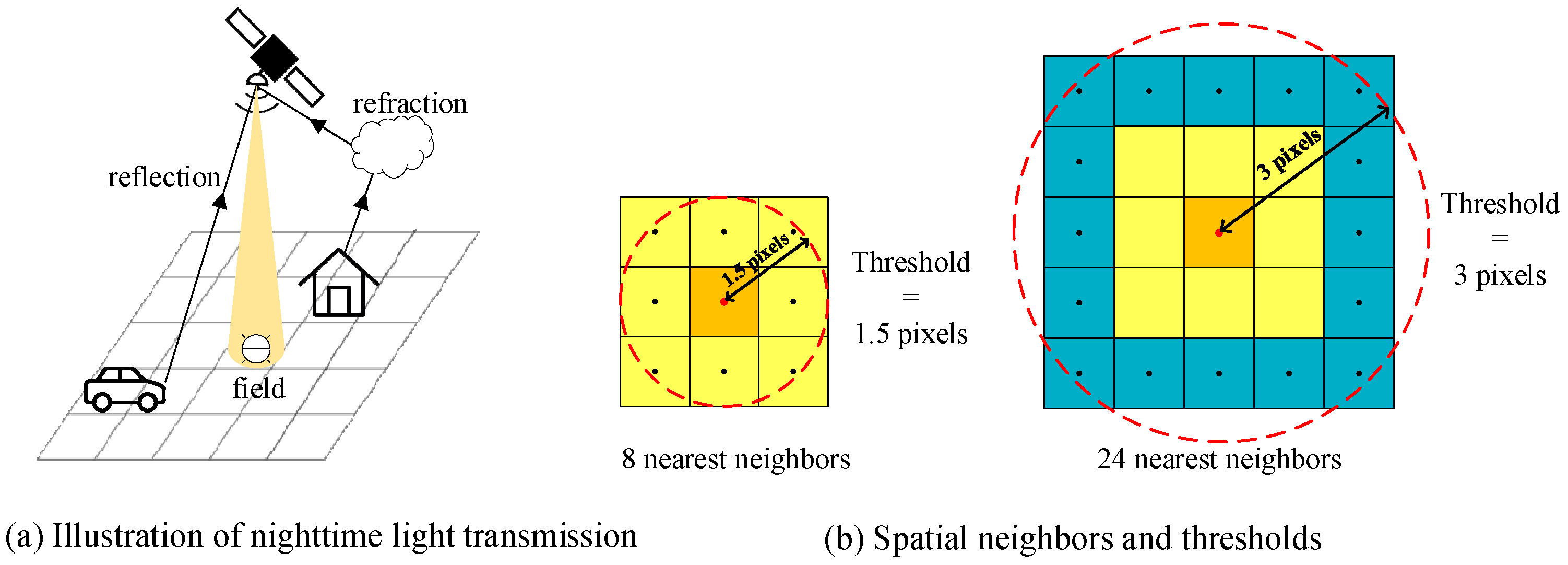
For the spatial autoregressive model, setting the spatial weight matrix W has a great influence on the regression results [45]. In this paper, k nearest neighbors was used to choose the adjacent pixels, and the inverse distance method was used to determine the weight of each neighboring pixel [46].

In order to specify the threshold of spatial neighbors, the influence range of spatial autocorrelation effects needs to be identified. The semi-variation coefficients are commonly used indicator to determine the most suitable k value. According to Chen’s study, the influence range of spatial autocorrelation characteristics is about 2–11 pixels for different land use types [47]. In this paper, we selected two k values (i.e., k = 8 and k = 24) to construct the spatial weight matrices and compare regression results for exploring the influence range and optimal threshold of spatial autocorrelation of night light data. The specified eight and 24 nearest neighbors are shown in Figure 3, which correspond to thresholds of 1.5 and three pixels, respectively. The weights for the pixels in the adjacent region to the central pixel are the reciprocal of their distances, while the weights for other pixels are set to 0.

2.2.3. Land Use Types Proportion Statistic

The nighttime light value of a pixel can be expressed as the sum of the brightness values of all land use types, which is calculated by multiplying the NLI of such a land use types with the proportion of it in the central pixel [33]. So, we counted the proportions of different land use types in each grid. Because of the autocorrelation of land use in geographical space, there were only a few land types that existing in the same pixel, which led to uneven proportions of land use types. This phenomenon incurs a sparse matrix solving problem in regression, which is solved by the modified models proposed in Section 2.3.2 and Section 2.3.3.

2.3. Spatial Autoregressive Model Construction

Because of the sensor resolution and landscape variability, remote sensing data exhibited a spectral dependency between neighboring pixels, i.e., spatial autocorrelation, in multispectral remote sensing images, and in nighttime light remote sensing data [48,49,50,51,52], which was also proved for our three study areas in

Table A1. Moran’s I of the coarse nighttime light images in the study areas.

City	Berlin	Massachusetts	Shenzhen
Moran’s I	0.766	0.971	0.833

of the Appendix A. Campbell used Landsat multi-spectral scanner images to study the positive autocorrelation between neighboring pixels [53]. Dana indicated that the radiance of one pixel can further affect the radiance of pixels 4–6 away [54]. The presence spatial autocorrelation violates the hypothesis that the data are independent, so traditional methods such as OLS and NOLS may yield unsatisfactory results and lead to errors in analyzing the cause of night light. Therefore, the accuracy of the relation between nighttime light and land use types could be improved by considering the spatial autocorrelation.

The main concern of this paper is the correlation between night light and land use. Studying the origin of the spatial autocorrelation of night light images can help us understand the spatial pattern of night light, which in turn expanding the application scope of night light images. Night light data are characterized in the single band by a low resolution and significant brightness overflow in general. Three potential reasons for the spatial autocorrelation phenomenon, which need to be eliminated, can be drawn as follows [53,54]: (1) the refraction and reflection of light (Figure 3a); (2) the influence of climate and atmospheric conditions; (3) positive correlation caused by the imaging system. The first explanation reflects that the night light brightness is affected by the ambient brightness. This part of autocorrelation comes from the dependent variable of luminous brightness itself, so it can be measured by the spatial lag model (SLM). The second and third explanations indicate that, besides being affected by the dependent variable, there are some factors missing in linear regression that are not related to the independent variable, and the spatial error model (SEM) can be used to solve this problem. Therefore, we analyzed application scenarios and the influenced the spatial ranges of the two models through further experiments in this paper.

2.3.1. Traditional Spatial Autoregressive Model

Because of the strong spatial autocorrelation within nighttime light images, the classical regression models are no longer applicable [55]. Spatial autoregressive models are an effective method with which to solve this problem, which include the first-order spatial auto-regressive model, spatial lag model and spatial error mode. Among these models, the spatial lag model and the spatial error model are the most widely used. The general form of the autoregressive models is as Equation (1).

$$\{\begin{array}{c}y= \rho W_{1}y+X\beta +\mu \\ \mu =\lambda W_2\mu +\epsilon \end{array}$$

(1)

where $y$ is the dependent variable; $X$ is an n-by-k independent variable matrix; $\beta$ is a k-by-1 parameter vector associated with the independent variable $X$. $W_1$ and $W_2$ are the n-by-n order weight matrixes, reflecting the spatial trend of the dependent variable and the spatial trend of residuals respectively; $\rho$ is the spatial lag variable W_y coefficient;$\lambda$ is the spatial correlation intensity between regression resistors. $\mu$ is a n-by-1 error vector and $\epsilon$ is a normally distributed random error vector [56].

Different spatial autoregressive models can be obtained by applying different model parameter restrictions. When $\rho \ne 0$ and $\lambda =0$, it is a SLM; when $\rho =0$ and $\lambda \ne 0$, it is a SEM. The SLM model considers dependent variables on a spatial object are related not only to independent variables on the same object, but also to dependent variables of adjacent objects. The SEM model assumes that spatial correlation is generated by missing variables. It reflects the error propagation process through the spatial covariance of different regions [50].

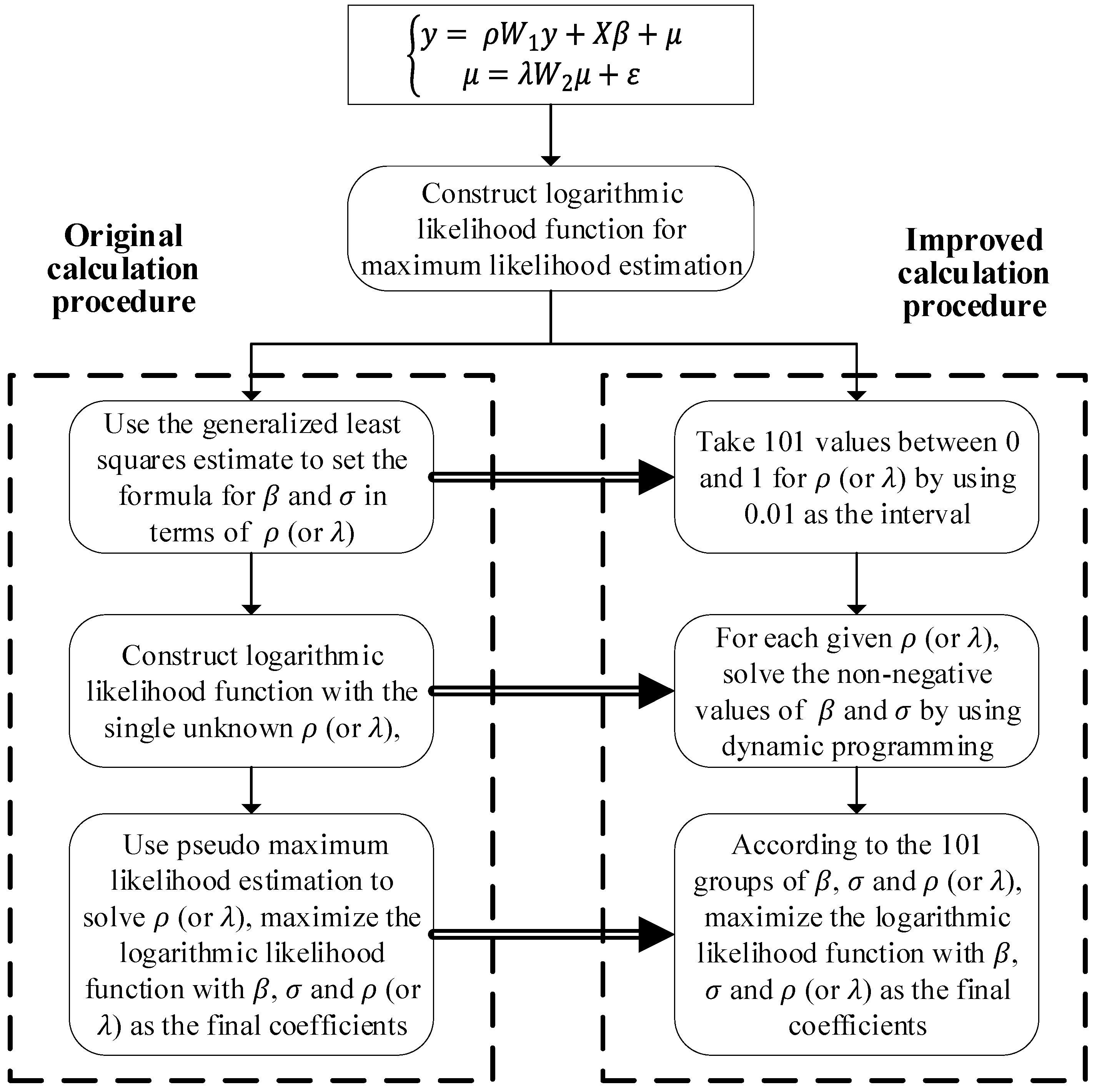
These models can measure the spatial autocorrelation caused by dependent variables and error, but have troubles in parameter interpretation and model solving. According to the physical meaning, the value of the land use brightness coefficient should be non-negative. However, the coefficients of the independent variables will contain both positive and negative values if following the conventional model’s procedure. It incurs difficulty to interpret the correlation between particular land use types and NLI. Meanwhile, the proportion of land use types in a single pixel is uneven due to the agglomeration of different land use types. It leads to a sparse coefficient matrix of the proportions, and impedes the solving of traditional spatial autoregressive model, in turn posing a great challenge to the analysis of the relation between land use and nighttime light. Therefore, we proposed an improved solving method by making the coefficients non-negative, which may better explain the correlations. Meanwhile, instead of using the original matrix inversion method, we adopted dynamic programming to solve the local optimal autoregressive coefficient using the multistage optimization decision method provided by MATLAB software. It enhances the robustness in solving even when the coefficient matrix is sparse. The improved calculation procedure is as illustrated in Figure 4.

2.3.2. Improved Non-Negative Spatial Lag Model (NSLM)

The spatial lag model can measure the spatial autocorrelation caused by the dependent variable. The regression equation is as Equation (2).

$$y=\rho Wy+X\beta +\epsilon$$

(2)

where y denotes the nighttime light value of the pixel, and the proportion of different land use types in this pixel i are denoted by {x_i1, x_i2, …, x_im}. n denotes the number of the pixels on nighttime light images, and m denotes the number of land use types. ${\beta }_j$ denotes the NLI of the land use type j. $\rho$ is the coefficient of spatial lag variable W_y, which is also called the spatial lag factor. W is the spatial weight matrix, which represents the influences between all pixel pairs in the image. $\epsilon$ is a normally distributed random error vector, which can be denoted as $\epsilon ~N\left(0,{\sigma }^2{I}_n\right)$.

In order to solve the three variables, i.e., $\beta , \rho$ and $\sigma$, a new vector $\theta =\left(\beta , \rho ,\sigma \right)$ is constructed. Maximum likelihood estimation is used to solve the variables according to the traditional spatial lag model. The logarithmic likelihood function of vector $\theta$ is shown in Equation (3).

$$lnL\left(\theta \right)=\frac{n}{2}\ln \left(2\pi \right)-\frac{n}{2}ln{\sigma }^2+ln\left|I_n-\rho W_n\right|-\frac{1}{2{\sigma }^2}{\left(y-\rho W_{n}y-X\beta \right)}^2$$

(3)

Since the value of spatial lag factor $\rho$ is usually between 0 and 1, to reduce the number of unknowns, we use the enumeration method and take 101 $\rho$ values between 0 and 1 by using 0.01 as the interval. For each given value of $\rho$, dynamic programming is used to solve the non-negative value of $\beta$ with constraints, and then $\rho$ and $\beta$ are used to solve the corresponding value of $\sigma$. The solution methods of $\beta$ and $\sigma$ are shown in Equations (4) and (5).

$$\widehat{\beta }=arg \underset{\beta }{\min }{\displaystyle \sum }{\Vert \rho W_{n}y+X\beta -y\Vert }^2 (\beta >0)$$

(4)

$${\sigma }^2=\frac{1}{n}{\left(\rho W_{n}y+X\beta -y\right)}^2$$

(5)

According to the 101 vectors of $\theta$, the logarithmic likelihood function of $\rho$ is calculated using Equation (6), and $\rho$ and $\beta$ that maximize the logarithmic likelihood function are obtained.

$$lnL\left(\rho \right)=\frac{n}{2}\ln \left(2\pi \right)-\frac{n}{2}ln{\sigma }^2+ln\left|I_n-\rho W_n\right|$$

(6)

2.3.3. Improved Non-Negative Spatial Error Model (NSEM)

The spatial error model is more accurate when spatial correlation is generated by neglected variables. It reflects the error propagation process through the spatial covariance of different regions. The regression equation is as Equation (7).

$$\mathrm{y}= X\beta +\mu , \mu =\lambda W\mu +\epsilon$$

(7)

where the weight matrix W reflects the spatial trend of residuals; $\lambda$ is the spatial correlation intensity between regression resistors; $\epsilon$ is the random error vector; and $\mu$ is a normally distributed random error vector. X, y and $\beta$ represent the same meaning as the NSLM.

As with the NSLM, the maximum likelihood estimation is used to solve the unknowns of the model by introducing a new vector $\tau =\left(\beta ,\lambda ,\sigma \right)$. The logarithmic likelihood function of the vector is shown in Equation (8).

$$lnL\left(\tau \right)=-\frac{n}{2}\ln \left(2\pi \right)-\frac{n}{2}ln{\sigma }^2+ln\left|I_n-\lambda W_n\right|-\frac{1}{2{\sigma }^2}{\left(\left(I_n-\lambda W_n\right)\left(y-X\beta \right)\right)}^2$$

(8)

The 101 values of the spatial lag factor $\lambda$ are also selected between 0 and 1 by using 0.01 as the interval. For each given value of $\lambda$, dynamic programming solves the non-negative value of $\beta$ with constraints, and the value of $\sigma$ is solved by using $\lambda$ and $\beta$. The solution methods of $\beta$ and $\sigma$ are shown in Equations (9) and (10). Then, according to the obtained vectors of $\tau$, the logarithmic likelihood function of $\lambda$ is calculated using Equation (11), and $\lambda$ and $\beta$ that maximize the logarithmic likelihood function are obtained.

$$\widehat{\beta }=arg \underset{\beta }{min}{{\displaystyle \sum }\Vert X\beta -y-\lambda W\mu \Vert }^2 (\beta >0)$$

(9)

$${\sigma }^2=\frac{1}{n}{\left(X\beta -y\right)}^2$$

(10)

$$lnL\left(\rho \right)=-\frac{n}{2}\left(\ln \left(2\pi \right)+1\right)-\frac{n}{2}ln{\sigma }^2+ln\left|I_n-\lambda W_n\right|$$

(11)

3. Results

3.1. Comparative Analysis of Nighttime Light Intensity

In order to verify the accuracy of our models, the estimated NLIs of each land use type from coarse-resolution nighttime light imagery by different models are compared with that of reference data listed in Table 1. For the proposed two non-negative spatial autoregressive models, NSEM and NSLM, the non-negative spatial linear regression model NSL without considering spatial autocorrelation was selected as the baseline method. In this experiment and the analysis in Section 3.2, spatial weight matrices constructed by the eight nearest neighbors were used as the case study.

Considering different reference data as described in Table 1, the calculations of NLIs in three study areas were different. In Berlin, the reference data, nighttime aerial photographs with 1 m resolution, has a higher resolution than the land use map. So, for each type of land use, the average value of NLI fell into the land use type on the map was calculated as the reference NLI value. In Massachusetts and Shenzhen, the reference data were photographs with 30 m resolution and 170m resolution, respectively, whose resolutions were lower than that of land use maps. To ensure the accuracy of the reference NLI data, land use proportion maps at a lower resolution were produced from the original land use map. For each land use type, the pixels that entirely occupied the land use type were treated as pure pixels, and the average nighttime light values of pure pixels were calculated as the reference NLI value. The estimated NLIs and reference NLIs in three study areas are listed in Table A1,

Table A2. NLIs of reference data (RD) and analysis data from different models in Massachusetts.

Land Use Type	NLI
	RD	NLS	NSLM	NSEM
cropland	11.36	0.00	0.00	0.00
pasture	11.99	0.00	0.00	0.00
forest	12.85	0.89	2.13	1.70
Non-forested wetland	14.07	9.37	11.48	7.82
mining	15.94	33.52	34.48	29.13
open land	17.75	0.00	0.00	0.00
participation recreation	34.13	86.80	108.24	100.59
spectator recreation	38.74	364.30	175.72	164.25
water-based recreation	20.58	180.08	0.00	0.00
multifamily residential	50.16	548.43	343.14	317.27
high-density residential	30.53	208.97	121.39	108.70
medium-density residential	23.44	142.87	84.93	76.24
low-density residential	14.14	95.47	53.28	48.34
saltwater wetland	17.54	18.02	8.75	6.99
commercial	54.78	518.58	288.65	278.79
industrial	41.73	344.00	212.82	198.07
transitional	25.43	0.00	23.87	14.60
transportation	40.99	186.06	177.23	162.82
waste disposal	30.32	45.11	21.42	6.23
water	18.3	8.44	16.13	13.37
cranberry bog	7.86	0.00	0.00	0.00
powerline/utility	17.91	150.29	113.26	102.56
saltwater sandy beach	18.11	41.15	0.00	0.00
golf course	18.97	173.68	79.84	71.98
marina	45.61	543.06	384.66	270.96
urban public/institutional	42.36	320.99	253.91	237.75
cemetery	29.34	160.30	150.27	129.58
orchard	12.58	70.35	42.39	39.27
nursery	14.06	33.15	30.33	27.00
forested wetland	11.91	59.17	40.67	36.56
very low density residential	12.43	0.00	0.00	0.00
junkyard	19.51	65.68	139.70	116.83
brushland/successional	16.92	0.00	0.00	0.00
regression R2	1	0.78	0.79	0.81

and

Table A3. NLIs of reference data and analysis data from different models in Berlin.

Land Use Type	NLI
	RD	NLS	NSLM	NSEM
Dense block-edge development	126.6	0	0.00	0.00
Closed block-edge development	134.4	25.2	9.08	19.25
Closed and half-open block-edge	121.6	0	0.00	0.00
Mixed development	124.9	23.5	8.67	15.46
Block-edge development with large courts	115.2	3	0.00	0.00
Row building with architecture row green space	116.2	9.8	0.00	0.00
Heterogeneous, inner-city mixed development	145.1	5.5	53.28	77.22
Vacated block-edge development	131.8	26.4	8.47	29.31
Storey residential building	131.8	25.5	26.53	45.33
Large residential areas and free-standing high-rise buildings	126.5	10.8	0.00	0.00
Row building with landscaped green settlement	116.1	10.3	0.00	2.35
Concentration in detached house areas	116.7	3.6	0.00	0.00
Rural mixed development	107	0	0.00	0.00
Vilas and urban villas with park-like garden	118.7	3	0.00	0.00
Row and duplex houses with yard	113.6	0.8	0.00	0.00
Freestanding single-family house with yard	115.2	1.7	0.00	0.00
Weekend houses and allotment garden-like areas	108.2	5.1	4.96	10.58
Core area	337.4	92.5	122.69	202.97
Small business and industry, large-scale retail area, high building density	194.5	19.1	18.24	26.76
Mixed area without character of residential area, high building density	173.7	79.3	46.45	81.89
Small business and industry, large-scale retail area, low building density	148.9	22.8	15.89	25.85
Mixed area without character of residential area, low building density	135.6	5	1.06	0.80
Utilities area	168	26.2	23.87	39.63
Railway station and railway system without railroad embankment	155.7	13.8	9.62	20.35
Railroad embankment	132.1	22	5.48	7.59
Parking lot	194.9	48.3	70.34	115.71
Other traffic area	178.6	17.1	17.24	27.92
Airport	257.4	39.4	17.97	30.72
Administration	184.9	57.9	40.42	81.35
Culture	219.4	57	74.57	132.27
Law enforcement	140.1	13.6	12.59	21.66
School, old buildings	119.2	0	0.00	0.00
School, new buildings	117.4	19.6	3.83	12.20
University and research	139.9	20.8	1.71	4.90
Child day care center	115.9	25	18.17	37.81
Other youth facilities	111.1	1.2	0.00	0.00
Campground	100.7	0	0.00	0.00
Other and heterogeneous public facilities and special areas	152.7	17.2	10.40	19.33
Church	253.2	75.7	80.32	118.69
Hospital	129	25.2	4.60	14.70
City square/promenade	284.1	128.9	142.24	208.46
Covered sports facilities	146.8	21	21.79	28.24
Uncovered sports facilities	124.1	15.8	3.06	8.09
Tree nursery/horticulture	106.2	5.9	0.00	2.78
Allotment garden area	108	11.5	2.71	7.76
Park, green area	111.2	17.1	1.69	7.50
Cemetery	105.6	15.2	4.33	10.56
Vacant area	105.6	7.2	0.00	0.00
Agriculture	178.6	17.1	17.24	27.92
Forest	101.9	3.5	0.73	2.04
Water	104.7	5.2	0.94	1.92
Street	164.9	31.9	20.71	35.45
regression R2	1	0.71	0.75	0.75

in the Appendix A. The differences between the nighttime brightness coefficients of different land use types in these tables indicated that land use type was an important factor affecting the NLI.

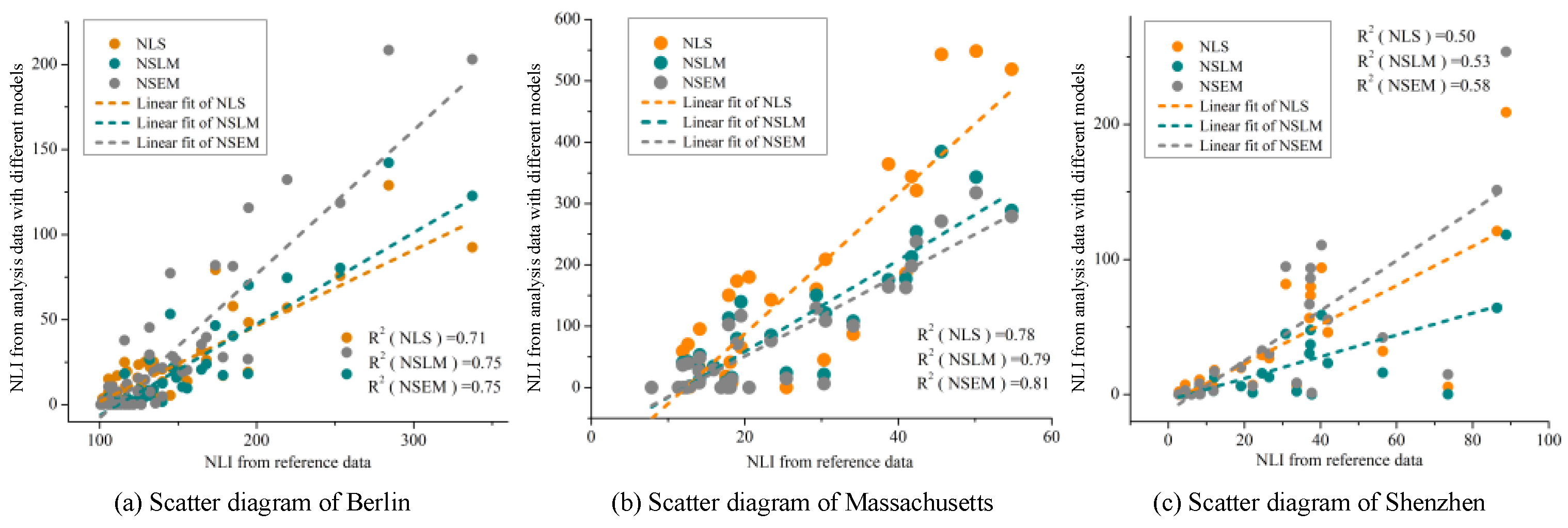
In order to compare the performance of the models, we adopted linear regression to analyze the fitting of NLI values for all land use types. As sensors are different, the NLI values represent different units of brightness among images. Therefore, the NLIs derived from different nighttime light images may vary on the same land use map and cannot be compared directly. Considering that there were 52, 32 and 26 land use types in three study areas respectively, the R² values were satisfactory, showing that the estimated NLIs from NPP/VIIRS data reflected the actual NLIs of different land use types. The higher goodness-of-fit indicated better estimation accuracy and better capability to reflect the relationships between NLI and land use types in our case [33]. Figure 5 shows the scatter diagrams and the linear regression results.

As illustrated in Figure 5, NSEM had the highest R² value of regression among the three models, while NLS had the lowest goodness of fit for all three study areas. We also found that the R² values in Shenzhen were lower than those of other two areas, as there is a three-year gap between the NPP/VIIRS imagery and LuoJia-01 imagery. However, R² values of NSLM and NSEM were still higher than NLS in Shenzhen, which demonstrated that the estimated NLI by NSLM and NSEM models was closer to reality. In general, NSLE and NSEM have a better performance for explaining the relationships between NLI and land use types.

The fitting confidence of the regression models in the three experimental areas were further evaluated via Akaike information criterion (AIC), which is widely used in factor analysis, regression and latent class analysis [57]. AIC is capable of taking both descriptive accuracy and parsimony into account [58]. AIC is defined as Equation (12).

$$AI{C}_i= -2\log L_i+2V_i$$

(12)

where $L_i$ is the maximum likelihood for model i, which is determined by adjusting the free parameters $V_i$ to maximize the probability to generate the data observed by the candidate model. The AIC values of NLS, NSL and NSE models are shown in

Table 2. Akaike information criterion (AIC) values of the three regression models in the three study areas.

Study Area	AIC
	NLS	NSLM	NSEM
Berlin	5462.47	4326.10	4358.73
Massachusetts	269,392.46	182,997.35	184,658.20
Shenzhen	62,316.81	56,429.73	56,482.67

.

From Table 2, we can see that AIC values of NSLM and NSEM were far less than that of NLS; there was no significant difference between NSLM and NSEM. It indicated that NSLM and NSEM had better performances by leveraging the accuracy and the complexity of the model, when compared with NLS. Although our models had more free parameters (i.e., spatial lag variable $\rho$ for NSLM), significant improvement in accuracy can be achieved. The AIC values of NSLM are slightly lower than those of NSEM, which may reflect that the spatial lag effect of NLI was more significant than the spatial error effect in the study areas. In addition to calculating the R² between the models and the reference data and the AIC value of the models, we also tested the significance of the regression coefficients (i.e., NLI) of each model. The land use types with large coefficients in the NSLM and NSEM models proposed generally had large t statistics, indicating that they had significant impacts on the brightness value of nighttime lights. Therefore, the proposed two models can measure the NLIs of different land use types more accurately so as to better understand the relationship between night light and land use.

3.2. Spatial Correlation of Residual Error Analysis

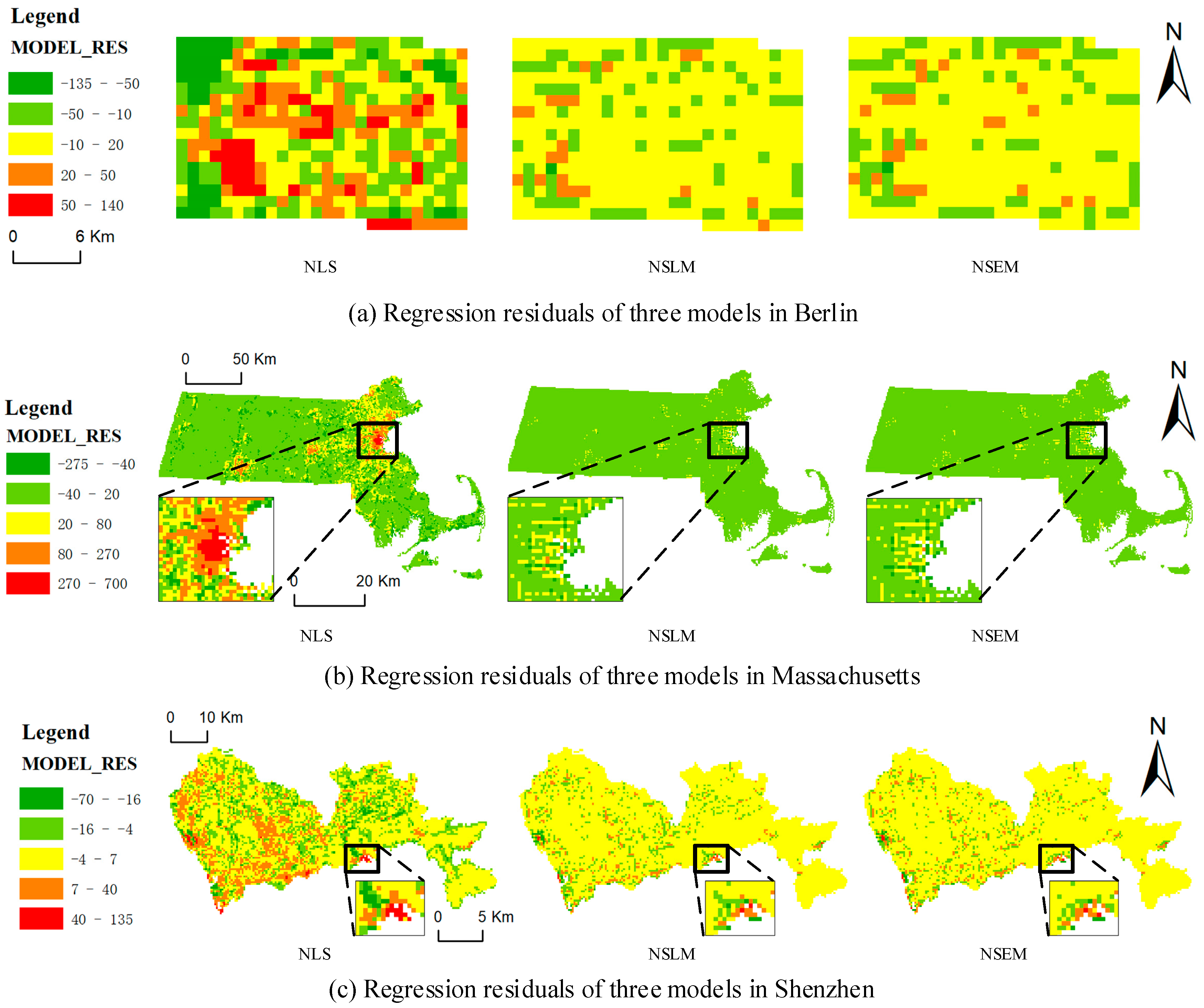
Since Moran’s I analysis in Table A1 of the Appendix A showed a significant spatial autocorrelation effect of the NLIs in the three study areas, the interpretation effect [59,60] on the spatial autocorrelation of NLI values for the three regression models was further compared via regression residuals. The residual within each pixel of different models was calculated by using the NLI of each global land use type and the proportion of land use of each pixel. The residual maps obtained are shown in Figure 6.

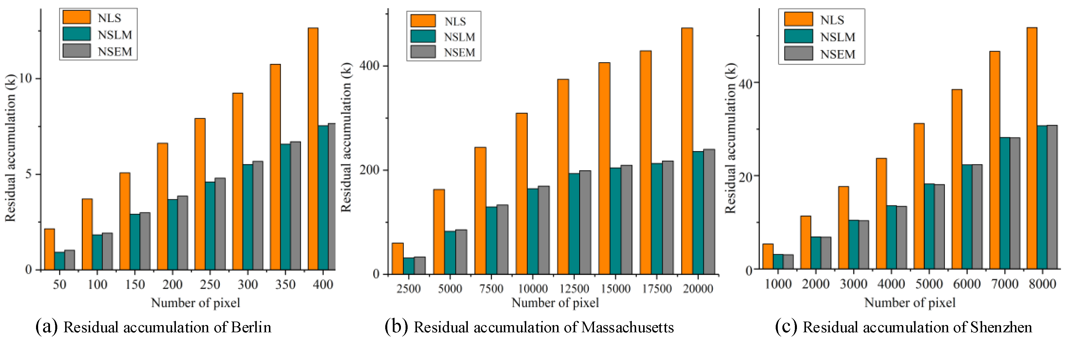
As shown in Figure 6, the regression residuals of NLS were larger than that of spatial autoregressive models, and the residuals were more concentrated in spatial distribution, showing a phenomenon of high–high and low–low aggregation. In order to quantitatively measure the interpretation effect of the three models on the global spatial autocorrelation effect, Moran’s I values and accumulation of the residuals of each model were calculated, as shown in

Table 3. Moran’s I values of regression residuals and residual accumulations in three study areas.

Study Areas	Moran’s I			Residual Accumulation
	NLS	NSLM	NSEM	NLS	NSLM	NSEM
Berlin	0.49	−0.11	−0.08	13,329.59	7887.78	8006.55
Massachusetts	0.64	0.23	0.15	495,257.68	246,287.95	250,681.10
Shenzhen	0.5	0.16	0.12	51,733.93	30,717.50	30,817.50

and Figure 7.

From Table 3, we can also find that Moran’s I values of the regression residuals by NLS were the highest in the three study areas, while those of NSLM and NSEM were much lower. Hence, NSLM and NSEM are more effective than NLS at eliminating the spatial autocorrelation effect of NLI. This result can also be found from the residual accumulation in Figure 7. In all three study areas, the accumulations of the absolute residuals of each pixel for NLS were much larger than those for NSLM and NSEM. This also indicated that NSLM and NSEM had a more accurate fitting effect on the relationship between land use and NLI.

4. Discussion

4.1. Nighttime Light Contribution of Urban Land Use Classes

From the NLIs of different land use types, we found that the major sources of nighttime light in the three areas varied, as illustrated in

Table A5. Top ten lightest and darkest land use types at night in the three study areas.

Top Ten Lightest Land Use Types at Night				Top Ten Darkest Land Use Types at Night
ID	Berlin	Massachusetts	Shenzhen	ID	Berlin	Massachusetts	Shenzhen
1	City square/promenade	Multifamily residential	Airport	11	Large residential areas and free-standing high-rise buildings	Waste disposal	Grassland
2	Core area	Commercial	Open storage yard	12	Concentration in detached house areas	Forest	Water
3	Culture	Marina	Industrial	13	Rural mixed development	Cropland	Mining
4	Church	Urban public/institutional	Parking lot	14	Vilas and urban villas with park-like garden	Pasture	Pool
5	Parking lot	Industrial	Street	15	Row and duplex houses with yard	Open land	Orchard
6	Mixed area without character of residential area, high building density	Spectator recreation	Railway	16	Freestanding single-family house with yard	Water-based recreation	Junkyard
7	Administration	Transportation	Multistory independent building	17	School, old buildings	Cranberry bog	Forest
8	Heterogeneous, inner-city mixed development	Cemetery	Spectator recreation	18	Other youth facilities	Saltwater sandy beach	Cropland
9	Storey residential building	Junkyard	High-density multistory building	19	Campground	Very low density residential	Nursery
10	Utilities area	High-density residential	Impervious surface	20	Vacant area	Brushland/successional	Levee

in the Appendix A. In Massachusetts, residential and commercial areas were the largest sources. Urban public facilities like the city squares and cultural areas were the lightest in Berlin. In Shenzhen, transportation and industrial areas were the main sources of nighttime light. The darkest parts of three study areas were also different. Old buildings and detached houses were darkest at night in Berlin, while in Massachusetts and Shenzhen, land covered with plants gave out the least light.

Different study areas have different types of brighter or darker land use, which may be due to the following reasons: (1) Different nations are at distinct stages of socioeconomic development. In developed countries, e.g., the United States and Germany, human activities at night mainly link with residential and commercial activities. So, residential land and commercial land use and urban public facilities have higher brightness in the night. On the other hand, China’s economy is in a stage of rapid development, and many metropolitan areas are vigorously carrying out urban sprawl, so infrastructure construction, transportation and industrial production are still very active in the night [61,62]. (2) Different countries have different policies on night lighting. Germany has stricter night lighting laws on nighttime light pollution and energy conservation than the United States, so night lighting is mainly concentrated in urban public facilities [10,63]. (3) The times of data collection were different. With development of the economic and technological progress, the role of different land use types in urban developments is gradually changing, and the amount of nighttime activities performed on them is changing accordingly.

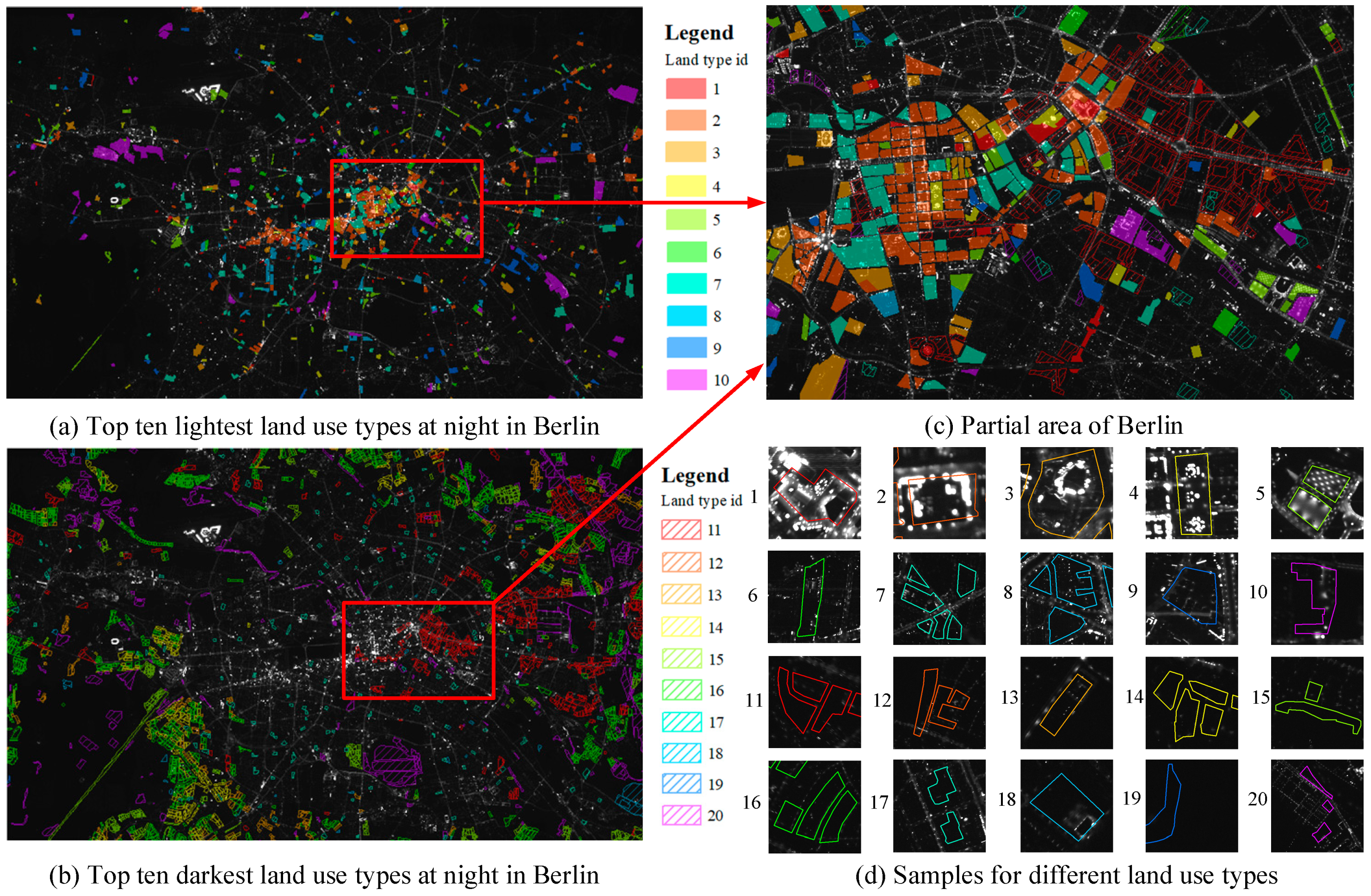
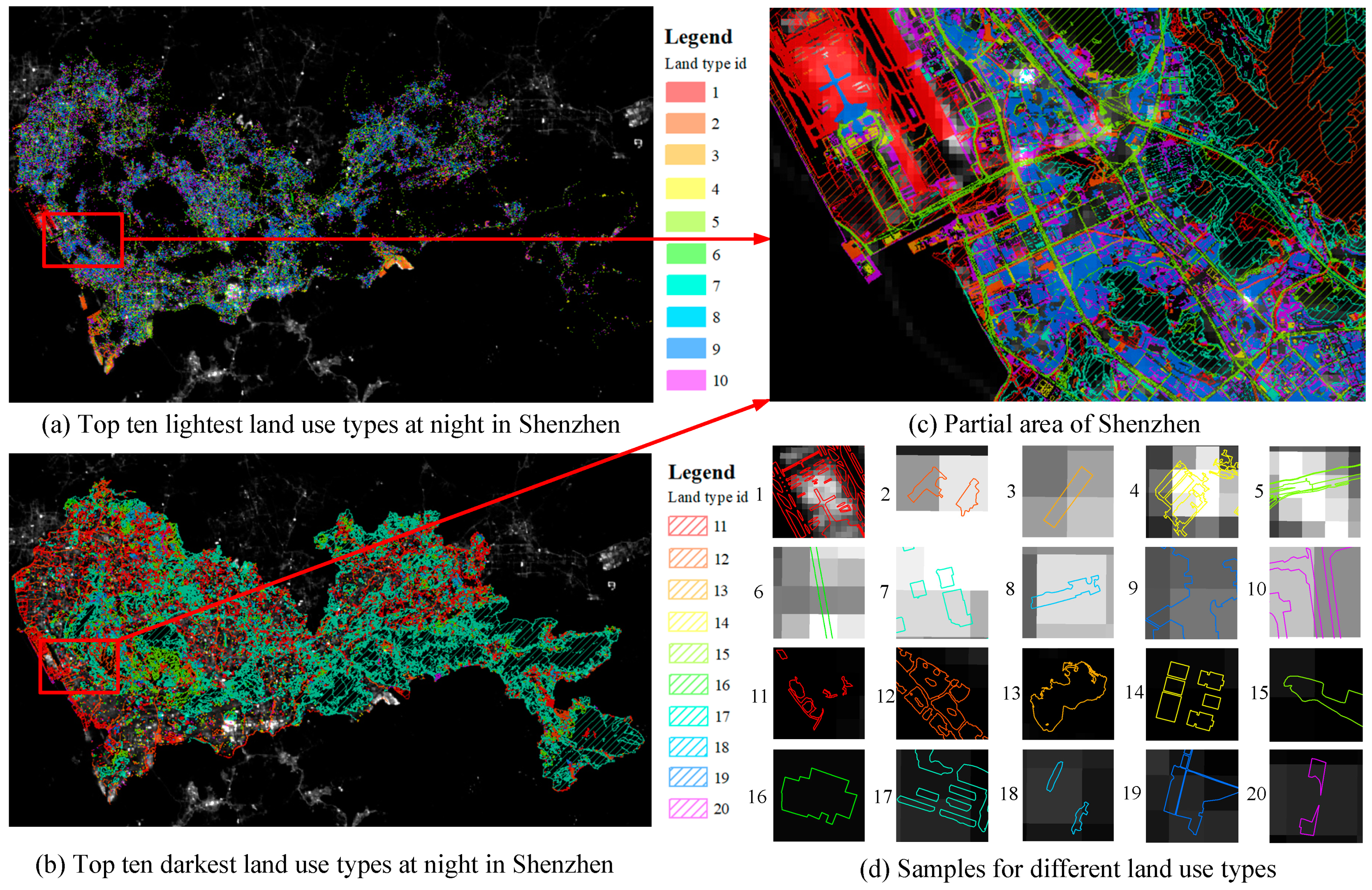
To intuitively illustrate the relationship between night lights on reference data and land use type, the top ten lightest and darkest land use types in Berlin through NLI calculated by NSLM (the land use types selected by NSEM and NSLM were same in the three areas) are shown in Figure 8, and the other two study areas are shown in Figure A1 and Figure A2 in the Appendix A.

From Figure 8 we can see that the land use type with large NLI was usually distributed in the bright area in the night light image, while the land use type with the smallest NLI was distributed in the dark area on the edge of the city. Therefore, our method can reflect the correlation between night light and land use, so as to better understand the component of night light. However, there are also some bright parts in the image that are not covered by specified land use types in Figure 8, which may be due to following reasons: (1) There is a difference between the acquisition time of land use and night light, and the areas with higher brightness may be new construction land. (2) NLI calculated by the proposed model reflects the global relationship between land use types and nighttime light. Even though some small areas had strong brightness values in the night light image, the average NLI for this land use type in the whole study area was low, so it was not identified as the top ten lightest. We may divide the study area into small patches to explore the relationships between NLI and land use type in different urban functional zones in future research.

4.2. Main Cause and Distance Threshold of Spatial Autocorrelation

The threshold of spatial autocorrelation effects and the setting of spatial weight matrixes have a great influence on the solution of the coefficient [45,47]. In order to analyze the application scenarios of NSLM and NSEM, different distance thresholds for calculating the spatial weight matrix were studied according to spatial neighborhood settings in Section 2.2.2. Since the image resolutions of Massachusetts, Berlin and Shenzhen were 1 km, 500 m and 500 m respectively, the distance thresholds of 1.5 pixels (k = 8) and three pixels (k = 24) of the three areas were different. R² values of linear fitting NLI values of various land use types were used to analyze the accuracies of the two models, and the results are shown in

Table 4. R² of linear fitting NLI values of two models under different distance thresholds.

Study Area	Distance threshold
	0.75 km		1.5 km		3 km
	NSLM	NSEM	NSLM	NSEM	NSLM	NSEM
Berlin	0.75	0.75	0.68	0.69	0.25	0.22
Massachusetts	/		0.79	0.81	0.63	0.56
Shenzhen	0.53	0.58	0.4	0.42	0.35	0.31

.

As illustrated in Table 4, with the increasing of the distance threshold, the fitting accuracy of the two models decreased significantly. This result shows that the eight first-order adjacent pixels had the greatest influence on the central pixel. A large threshold may degrade the fitting and even generated worse results than the traditional NLS model. This phenomenon indicated that the spatial autocorrelation effect of the night light image had a certain distance threshold, and an overlarge threshold will introduce noise and weaken the weight of the current pixel. Therefore, when studying the correlation between NLI and land use, the distance threshold needs to be carefully considered.

In addition, we also found that when the distance threshold was less than 1.5 km, the fitting accuracy of NSEM was higher than that of NSLM; when the distance threshold was greater than 1.5 km, NSLM had better performance. The difference in the model performance within and beyond the 1.5 km bandwidth may be due to the difference in the dominant role of spatial autocorrelation characteristics. The spatial autocorrelation in the spatial lag model is mainly derived from the dependent variable, while the spatial autocorrelation in the spatial error model is mainly derived from the error, or the independent variable not considered [64,65]. The sensor radiation characteristics or meteorological conditions may be the main contributors to spatial autocorrelation within the distance threshold of 1.5 km, while when the distance threshold is greater than 1.5 km, the dependent variable related to light refraction and reflection may be the dominant factor. The findings from the above experiments may provide guidelines for selecting regression models. When the resolution of night light data is high, the spatial error model may get a better fitting effect. When the resolution of night light data is low, priority should be given to the spatial lag model.

4.3. Potential Use Case

The data sources, acquisition time and classification accuracy values of the three study areas were different, so NLIs of the same land use types obtained cannot be compared. In order to study the differences between NLIs of the same land use types in different regions and their influencing factors, we used Finer Resolution Observation and Monitoring of Global Land Cover (FROM-GLC) 2015 data (http://data.ess.tsinghua.edu.cn/fromglc2015_v1.html) from Tsinghua University and the NPP/VIIRS nighttime light images to solve the NLI of each land use type in different cities in China by using NSEM with threshold of the eight nearest neighbors.

FROM-GLC maps are the first 30 m resolution global land cover maps produced using Landsat Thematic Mapper (TM) and Enhanced Thematic Mapper Plus (ETM+) data. We used NSEM to calculate the NLIs of seven first-level classifications of land uses in five provincial capital cities in China. These cities are located in different regions of China with different levels of economic development, which can help us find the relation between NLIs of land use types and economic development. The estimated NLIs are listed in

Table 5. Estimated NLIs of the five provincial capital cities in China.

Land Use Type	Shenzhen	Shanghai	Wuhan	Taiyuan	Harbin
Cropland	20.08	8.40	2.60	2.07	0.17
Forest	8.05	6.53	1.18	0.17	0.07
Grass	19.96	11.05	8.14	0.79	0.51
Shrub	9.95	10.79	0.86	0.14	0.06
Wetland	28.75	8.60	3.57	2.20	0.08
Water	17.41	2.99	2.78	4.85	0.56
Impervious surface	31.34	29.16	24.16	21.43	9.37
Bare land	41.45	16.55	20.63	5.67	1.83

.

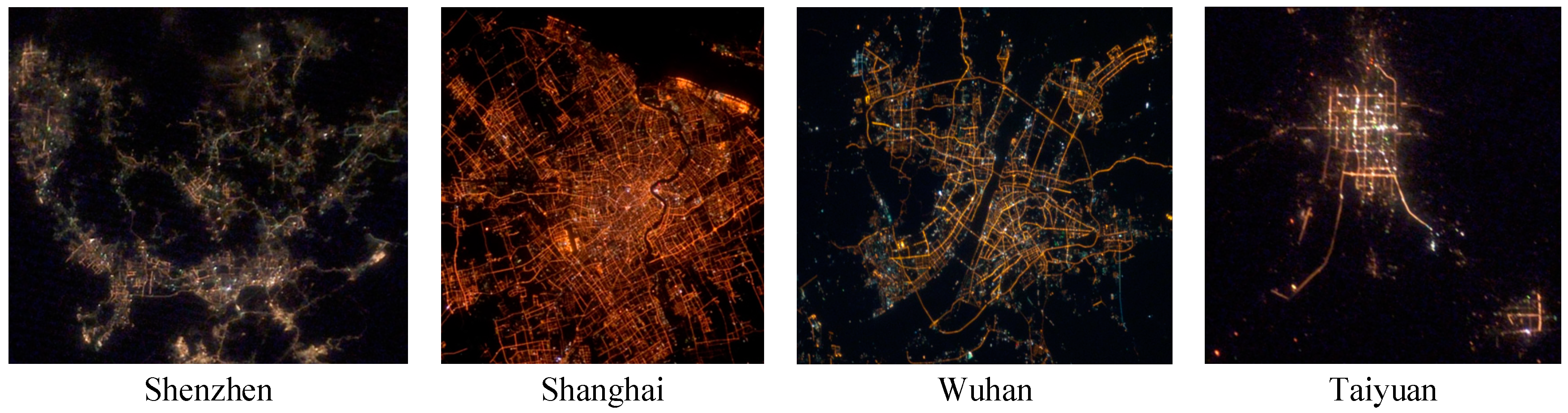
As shown in Table 5, there were significant differences in the NLI for each land use type between different cities. All land use types in Shenzhen and Shanghai had higher brightness values, while those in Taiyuan and Harbin were lower. By observing NLIs of the same land use types in different cities, we found that forests and shrubs had relatively small NLIs in each city, while impervious surfaces and bare land had large NLIs. Shenzhen was the only city for which bare land had the largest NLIs; meanwhile impervious surfaces were the lightest land use type in other cities. Moreover, bare land and impervious surfaces had relatively close NLIs in Shenzhen, Shanghai and Wuhan; the brightness of impervious surfaces was significantly higher than those values of other land use types in Taiyuan and Harbin.

This phenomenon may reflect the different development speeds and stages of different cities, and Nighttime photographs from the International Space Station shown in Figure 9 can help explain it. Shenzhen is in the midst of rapid urban expansion. The bare lands in the suburbs of the city are construction sites and, therefore, have a higher brightness than the built impermeable surfaces. However, Taiyuan and Harbin have had relatively slow or even stagnant urban expansion in recent years [66,67,68]. Most of the bare lands were stagnant construction land or cultivated land, so the brightness was far lower than for the impervious surfaces.

To verify our observation and compare the stage of urban construction, official statistics of the experimental cities [69,70,71,72] were also collected. Harbin was not included in the comparison due to the administrative division adjustment in 2015. The investment completed in the current year and the cost of new construction in 2015 were chosen to study the urban construction situation, which are shown in

Table 6. Index of urban construction in the four experimental cities.

City	Shenzhen	Shanghai	Wuhan	Taiyuan
Area (Square Kilometer)	1997	6341	8596	1500
Investment Completed in Current Year (100 million Yuan)	3298.31	2880.45	7680.89	2025.60
Cost of New Construction (100 million Yuan)	2521.82	1837.92	3306.86	1016.50
Proposition of New Construction in all investment	76%	64%	43%	50%

. As we can see from the table, new construction projects in Shenzhen and Shanghai accounted for a large proportion in the total investment, about 76% and 64% respectively. This indicated that the urban constructions in Shenzhen and Shanghai were dominated by new construction projects, and plenty of bare lands were under construction in 2015. This is consistent with the modeling and analysis of night light data. Although the proposition of new construction investment in Wuhan is relatively small, the total amount is much higher than those values of other cities. Therefore, the urban sprawl speed is relatively fast in Wuhan, and the bare land may have a higher luminous brightness. In contrast, the new construction projects in Taiyuan accounted for a relatively low proportion in the total investment, and the total cost of new construction is also small compared with Shenzhen, which has a similar area, indicating that urban sprawl does not play a prominent role in Taiyuan.

The above analysis demonstrates that the NLIs calculated by our models can reflect the relation between land use types and night light more accurately than an NLS model with an appropriate distance threshold, and it is helpful to identify urban construction situations. It can better reveal the difference in the contribution of land use to night light so as to discover the differences in economic development stages and night light policies (Section 4.1) between different regions. Moreover, our models could facilitate other potential applications, such as light pollution prevention, traffic volume estimation and GDP composition. For example, when the land use types are of high classification accuracy, the contributions of different buildings types to nighttime brightness can be identified, and they could assist in establishing environmental policies for preventing light pollution in urban residential areas and ecological protection areas. When transportation land types are known in detail, the traffic volume of different transportation modes can be estimated according to NLI. In conclusion, the proposed regression models could be extended in different application scenarios to interpret the influences of human activities on nighttime light.

5. Conclusions

This study proposed two non-negative spatial autoregressive models to study the correlation of night light with land use types, which used a space adjacency matrixes to consider the spatial autocorrelation effect of nighttime light remote sensing data. Analysis of influential factors in the spatial autocorrelation effect provides a reference for model selection and adjacency matrix parameter setting. Compared with the traditional NLS model, the results of our models are closer to the verified data in the three study areas with the distance threshold of 1.5 pixels. The regression residual and its spatial autocorrelation issue are better eliminated. Meanwhile, the empirical experiments verified that the main source of night light varied in countries and regions due to different levels of economic development. In economically developed countries and regions, commercial land, public facilities and residential land have high brightness; in regions with rapid economic development, traffic, construction and industrial land are the main sources of nighttime light. Therefore, the proposed models can quantify the relation between nighttime light data and land use more accurately, and in turn benefit applications of nighttime light data in light pollution control, traffic volume estimation and urbanization stage analysis.

The paper also has the following shortcomings. (1) The NLIs of surface features were solved as homogeneous global variables in each study area. The value of each pixel in the same land use type may have great variance. So, the proposed method lacks a fine-grained analysis of the difference of NLIs within the same land use types. (2) Results of our models are greatly influenced by experimental data. Experimental dataset of land use have different classification standards, and the acquisition time varies greatly, so the results cannot be used for the comparison between these areas exactly. In order to obtain a generic conclusion on causes of nighttime lighting, further experiments are needed with the support of accurate and detailed experimental data.

References

- Welch, R. Monitoring urban population and energy utilization patterns from satellite data. Remote Sens. Environ. 1980, 9, 1–9. [Google Scholar] [CrossRef]
- Elvidge, C.D.; Baugh, K.E.; Kihn, E.A.; Kroehl, H.W.; Davis, E.R.; Davis, C.W. Relation between satellites observed visible-near infrared emissions, population, economic activity and electric power consumption. Int. J. Remote Sens. 1997, 6, 1373–1379. [Google Scholar] [CrossRef]
- Shi, K.; Yu, B.; Huang, Y.; Hu, Y.; Yin, B.; Chen, Z.; Chen, L.; Wu, J. Evaluating the Ability of NPP-VIIRS Nighttime Light Data to Estimate the Gross Domestic Product and the Electric Power Consumption of China at Multiple Scales: A Comparison with DMSP-OLS Data. Remote Sens. 2014, 6, 1705–1724. [Google Scholar] [CrossRef] [Green Version]
- Zhuo, L.; Ichinose, T.; Zheng, J.; Chen, J.; Shi, P.J.; Li, X. Modelling the population density of China at the pixel level based on DMSP/OLS non-radiance-calibrated night-time light images. Int. J. Remote Sens. 2009, 30, 1003–1018. [Google Scholar] [CrossRef]
- Bagan, H.; Yamagata, Y. Analysis of urban growth and estimating population density using satellite images of nighttime lights and land-use and population data. Gisci. Remote Sens. 2015, 52, 765–780. [Google Scholar] [CrossRef]
- Liu, Z.; He, C.; Zhang, Q.; Huang, Q.; Yang, Y. Extracting the dynamics of urban expansion in China using DMSP-OLS nighttime light data from 1992 to 2008. Landsc. Urban Plan. 2012, 106, 62–72. [Google Scholar] [CrossRef]
- Keola, S.; Andersson, M.; Hall, O. Monitoring Economic Development from Space: Using Nighttime Light and Land Cover Data to Measure Economic Growth. World Dev. 2015, 66, 322–334. [Google Scholar] [CrossRef]
- Liu, J.; Li, W. A nighttime light imagery estimation of ethnic disparity in economic well-being in mainland China and Taiwan (2001–2013). Eurasian Geogr. Econ. 2014, 55, 691–714. [Google Scholar] [CrossRef]
- Feng, J.; Bai, L.; Wang, K.; Zhang, X.; Xie, N.; Ran, Q.; Guo, M.; Xu, L. Analysis of Spatial Pattern of Urban System along the Overland Silk Road Economic Belt Using DMSP-OLS Nighttime Light Data. IOP Conf. Ser. Earth Environ. Sci. 2017, 57, 012052. [Google Scholar] [CrossRef]
- Kyba, C.; Garz, S.; Kuechly, H.; de Miguel, A.; Zamorano, J.; Fischer, J.; Hölker, F. High-Resolution Imagery of Earth at Night: New Sources, Opportunities and Challenges. Remote Sens. 2014, 7, 1–23. [Google Scholar] [CrossRef] [Green Version]
- Ma, T. Multi-Level Relationships between Satellite-Derived Nighttime Lighting Signals and Social Media–Derived Human Population Dynamics. Remote Sens. 2018, 10, 1128. [Google Scholar] [CrossRef] [Green Version]
- Zhao, M.; Cheng, W.; Zhou, C.; Li, M.; Wang, N.; Liu, Q. GDP Spatialization and Economic Differences in South China Based on NPP-VIIRS Nighttime Light Imagery. Remote Sens. 2017, 9, 673. [Google Scholar] [CrossRef] [Green Version]
- Li, X.; Wang, X.; Zhang, J.; Wu, L. Allometric scaling, size distribution and pattern formation of natural cities. Palgrave Commun. 2015, 15017. [Google Scholar] [CrossRef]
- Nakayama, Y.; Tanaka, S.; Mitsugi, R. An analysis of characteristics for change in night light distribution from 1980s to 1990s by the time series global dmsp mosaic data. In Proceedings of the 34th COSPAR Scientific Assembly, Houston, TX, USA, 10–19 October 2002. [Google Scholar]
- Yu, B.; Shu, S.; Liu, H.; Song, W.; Wu, J.; Wang, L.; Chen, Z. Object-based spatial cluster analysis of urban landscape pattern using nighttime light satellite images: A case study of China. Int. J. Geogr. Inf. Sci. 2014, 28, 2328–2355. [Google Scholar] [CrossRef]
- Li, D.; Yu, H.; Li, X. The Spatial-Temporal Pattern Analysis of City Development in Countries along the Belt and Road Initiative Based on Nighttime Light Data. Wuhan Daxue Xuebao (Xinxi Kexue Ban)/Geomat. Inf. Sci. Wuhan Univ. 2017, 42, 711–720. [Google Scholar]
- Han, P.; Huang, J.; Li, R.; Wang, L.; Hu, Y.; Wang, J.; Huang, W. Monitoring Trends in Light Pollution in China Based on Nighttime Satellite Imagery. Remote Sens. 2014, 6, 5541–5558. [Google Scholar] [CrossRef] [Green Version]
- Bennie, J.; Davies, T.W.; Duffy, J.P.; Inger, R.; Gaston, K.J. Contrasting trends in light pollution across Europe based on satellite observed night time lights. Sci. Rep. 2014, 4, 3789. [Google Scholar] [CrossRef] [Green Version]
- Cao, Z.; Wu, Z.; Kuang, Y.; Huang, N.; Wang, M. Coupling an Intercalibration of Radiance-Calibrated Nighttime Light Images and Land Use/Cover Data for Modeling and Analyzing the Distribution of GDP in Guangdong, China. Sustainability 2016, 8, 108. [Google Scholar] [CrossRef] [Green Version]
- Garrido-Jiménez, F.J.; Magrinyá, F.; del Moral-Ávila, M.C.; Rodríguez-García, G. The Relationship Between Urban Morphology and Street Lighting Operating Costs: Evidence from Medium-sized Spanish Cities. Appl. Spat. Anal. Policy 2017, 10, 381–399. [Google Scholar] [CrossRef]
- Imhoff, M. Using nighttime DMSP/OLS images of city lights to estimate the impact of urban land use on soil resources in the United States. Remote Sens. Environ. 1997, 59, 105–117. [Google Scholar] [CrossRef]
- Chen, Q.; Hou, X.; Zhang, X.; Ma, C. Improved GDP spatialization approach by combining land-use data and night-time light data: A case study in China’s continental coastal area. Int. J. Remote Sens. 2016, 37, 4610–4622. [Google Scholar] [CrossRef] [Green Version]
- Tan, M.; Li, X.; Li, S.; Xin, L.; Wang, X.; Li, Q.; Li, W.; Li, Y.; Xiang, W. Modeling population density based on nighttime light images and land use data in China. Appl. Geogr. 2018, 90, 239–247. [Google Scholar] [CrossRef]
- Small, C. Global population distribution and urban land use in geophysical parameter space. Earth Interact. 2004, 8, 1–18. [Google Scholar] [CrossRef]
- Gaston, K.J.; Bennie, J.; Davies, T.W.; Hopkins, J. The ecological impacts of nighttime light pollution: A mechanistic appraisal. Biol. Rev. 2013, 88, 912–927. [Google Scholar] [CrossRef]
- Cheng, X.; Shao, H.; Li, Y.; Wang, Y.; Yuan, Y. Evaluation model of urban land intensive use based on nighttime light remote sensing data. Trans. Chin. Soc. Agric. Eng. 2018, 34, 262–267. [Google Scholar]
- Kim, M.; Hong, S.H. Relationship between the reflected brightness of artificial lighting and land-use types: A case study of the University of Arizona campus. Landsc. Ecol. Eng. 2015, 11, 39–45. [Google Scholar] [CrossRef]
- Kuechly, H.U.; Kyba, C.M.; Ruhtz, T.; Lindemann, C.; Wolter, C.; Fischer, J.; Hölker, F. Aerial survey and spatial analysis of sources of light pollution in Berlin, Germany. Remote Sens. Environ. 2012, 126, 39–50. [Google Scholar] [CrossRef]
- Elvidge, C.D.; Baugh, K.E.; Dietz, J.B.; Bland, T.; Sutton, P.C.; Kroehl, H.W. Radiance Calibration of DMSP-OLS Low-Light Imaging Data of Human Settlements. Remote Sens. Environ. 1999, 68, 77–88. [Google Scholar] [CrossRef]
- Wei, Y.; Pan, L.; Guo, H. Semi-supervised learning via nonnegative least squares regression. In Proceedings of the 7th International Conference on Internet Multimedia Computing and Service, Zhangjiajie, China, 19–21 August 2015. [Google Scholar]
- Pan, C.; Bai, J.; Yang, G.; Wong, D.S.; Jang, S. An inferential modeling method using enumerative PLS based nonnegative garrote regression. J. Process. Control. 2012, 22, 1637–1646. [Google Scholar] [CrossRef]
- Groenen, P.J.F.; van Os, B.J.; Meulman, J.J. Optimal scaling by alternating length-constrained nonnegative least squares, with application to distance-based analysis. Psychometrika 2000, 65, 511–524. [Google Scholar] [CrossRef]
- Li, X.; Ge, L.; Chen, X. Quantifying Contribution of Land Use Types to Nighttime Light Using an Unmixing Model. IEEE Geosci. Remote Sens. Lett. 2014, 11, 1667–1671. [Google Scholar] [CrossRef]
- Sun, W.; Zhang, X.; Wang, N.; Cen, Y. Estimating Population Density Using DMSP-OLS Night-Time Imagery and Land Cover Data. IEEE J. Sel. Top. Appl. Earth Obs. Remote Sens. 2017, 10, 2674–2684. [Google Scholar] [CrossRef]
- Yang, X.; Yue, W.; Gao, D. Spatial improvement of human population distribution based on multi-sensor remote-sensing data: An input for exposure assessment. Int. J. Remote Sens. 2013, 34, 5569–5583. [Google Scholar] [CrossRef]
- Song, G.; Yu, M.; Liu, S.; Zhang, S. A dynamic model for population mapping: A methodology integrating a Monte Carlo simulation with vegetation-adjusted night-time light images. Int. J. Remote Sens. 2015, 36, 4054–4068. [Google Scholar] [CrossRef]
- Ma, T. Quantitative responses of satellite-derived night-time light signals to urban depopulation during Chinese New Year. Remote Sens. Lett. 2019, 10, 139–148. [Google Scholar] [CrossRef]
- Zhan, X.; Pan, W.; Zheng, P.; Cai, Y. Spatial correlation analysis of GDP at township scale of Fujian based on nighttime light data. In Proceedings of the International Workshop on Earth Observation & Remote Sensing Applications, Guangzhou, China, 4–6 July 2016; IEEE: Piscataway, NJ, USA, 2016. [Google Scholar]
- Zhang, F.; Zhang, X. Landscape spatial autocorrelation analysis of TM remote sensing data: A case study of Changping District, Beijing, China. Acta Ecol. Sin. 2004, 24, 2853–2858. [Google Scholar]
- Statistical Report: Residents in the state of Berlin on 31 December 2018; Tastomat Druck GmbH: Berlin-Brandenburg, Germany, 2018; pp. 4, 13, 18–22. Available online: https://www.statistik-berlin-brandenburg.de/produkte/kleinestatistik/AP_KleineStatistik_EN_2018_BE.pdf (accessed on 2 December 2019). (In German).
- Available online: https://www.census.gov/quickfacts/MA (accessed on 2 December 2019).
- Shenzhen Statistics Bureau. Shenzhen Statistical Yearbook 2017; China Statistical Press: Beijing, China, 2018. (In Chinese) [Google Scholar]
- Elvidge, C.D.; Baugh, K.; Zhizhin, M.; Hsu, F.C.; Ghosh, T. VIIRS night-time lights. Int. J. Remote Sens. 2017, 38, 5860–5879. [Google Scholar] [CrossRef]
- Hamylton, S.; Spencer, T.; Hagan, A.B. Spatial modelling of benthic cover using remote sensing data in the Aldabra lagoon, western Indian Ocean. Mar. Ecol. Prog. Ser. 2012, 460, 35–47. [Google Scholar] [CrossRef] [Green Version]
- Kelejian, H.H.; Prucha, I.R. A Generalized Spatial Two-Stage Least Squares Procedure for Estimating a Spatial Autoregressive Model with Autoregressive Disturbances. J. Real Estate Financ. Econ. 1998, 17, 99–121. [Google Scholar] [CrossRef]
- Li, H.; Calder, C.A.; Cressie, N. Beyond Moran’s I: Testing for Spatial Dependence Based on the Spatial Autoregressive Model. Geogr. Anal. 2007, 39, 357–375. [Google Scholar] [CrossRef]
- Chen, Y.X.; Qin, K.; Liu, Y.; Gan, S.Z.; Zhan, Y. Feature modelling of high resolution remote sensing images considering spatial autocorrelation. ISPRS Int. Arch. Photogramm. Remote Sens. Spat. Inf. Sci. 2012, XXXIX-B3, 467–472. [Google Scholar] [CrossRef] [Green Version]
- Chen, D.; Wei, H. The effect of spatial autocorrelation and class proportion on the accuracy measures from different sampling designs. ISPRS J. Photogramm. 2009, 64, 140–150. [Google Scholar] [CrossRef]
- Akcay, H.G.; Aksoy, S. Automatic Detection of Geospatial Objects Using Multiple Hierarchical Segmentations. IEEE Trans. Geosci. Remote Sens. 2008, 46, 2097–2111. [Google Scholar] [CrossRef]
- Hale, J.D.; Gemma, D.; Fairbrass, A.J.; Matthews, T.J.; Rogers, C.D.; Sadler, J.P. Mapping Lightscapes: Spatial Patterning of Artificial Lighting in an Urban Landscape. PLoS ONE 2013, 8, e61460. [Google Scholar] [CrossRef] [PubMed] [Green Version]
- Dominoni, D.; Quetting, M.; Partecke, J. Artificial light at night advances avian reproductive physiology. Proc. R. Soc. B Biol. Sci. 2013, 280, 20123017. [Google Scholar] [CrossRef] [Green Version]
- Levin, N.; Duke, Y. High spatial resolution night-time light images for demographic and socio-economic studies. Remote Sens. Environ. 2012, 119, 1–10. [Google Scholar] [CrossRef]
- Campbell, J.B. Spatial Correlation Effects upon Accuracy of Supervised Classification of Land Cover. Photogramm. Eng. Remote Sens. 1981, 47, 313–329. [Google Scholar]
- Dana, R.W. Background reflectance effects in Landsat data. Appl. Opt. 1982, 21, 4106–4111. [Google Scholar] [CrossRef]
- Dubin, R.; Pace, R.K.; Thibodeau, T.G. Spatial Autoregression Techniques for Real Estate Data. J. Real Estate Lit. 1999, 7, 79–96. [Google Scholar] [CrossRef]
- Anselin, L. Spatial Econometrics: Methods and Models; Springer: Haarlem, The Netherlands, 1988. [Google Scholar]
- Legendre, P. Spatial Autocorrelation: Trouble or New Paradigm? Ecology 1993, 74, 1659–1673. [Google Scholar] [CrossRef]
- Wagenmakers, E.J.; Farrell, S. AIC model selection using Akaike weights. Psychon. Bull. Rev. 2004, 11, 192–196. [Google Scholar] [CrossRef] [PubMed]
- Cliff, A.; Ord, K. Testing for Spatial Autocorrelation Among Regression Residuals. Geogr. Anal. 1972, 4, 267–284. [Google Scholar] [CrossRef]
- Mardia, K.V.; Marshall, R.J. Maximum Likelihood Estimation of Models for Residual Covariance in Spatial Regression. Biometrika 1984, 71, 135–146. [Google Scholar] [CrossRef]
- Wu, Y.; Zhu, Q.; Zhu, B. Comparisons of decoupling trends of global economic growth and energy consumption between developed and developing countries. Energy Policy 2018, 116, 30–38. [Google Scholar] [CrossRef]
- Wang, H.; Yang, Y.; Keller, A.A.; Li, X.; Feng, S.; Dong, Y.N.; Li, F. Comparative Analysis of Energy Intensity and Carbon Emissions in Wastewater Treatment in USA, Germany, China and South Africa. Appl. Energy 2016, 184, 873–881. [Google Scholar] [CrossRef] [Green Version]
- Sutton, P. Census from Heaven: An estimate of the global human population using night-time satellite imagery. Int. J. Remote Sens. 2001, 22, 3061–3076. [Google Scholar] [CrossRef]
- Lambert, D.M.; Brown, J.P.; Florax, R.J.G.M. A two-step estimator for a spatial lag model of counts: Theory, small sample performance and an application. Reg. Sci. Urban Econ. 2010, 40, 241–252. [Google Scholar] [CrossRef] [Green Version]
- Zimmerman, D.L.; Cressie, N. Mean squared prediction error in the spatial linear model with estimated covariance parameters. Ann. Inst. Stat. Math. 1992, 44, 27–43. [Google Scholar] [CrossRef]
- Liu, F.; Zhang, Z.; Shi, L.; Wang, X. Urban expansion modes of major cities in China in the past four decades. In Proceedings of the International Workshop on Earth Observation & Remote Sensing Applications, Guangzhou, China, 4–6 July 2016; IEEE: Piscataway, NJ, USA, 2016. [Google Scholar]
- Xu, M.; He, C.; Liu, Z.; Dou, Y. How Did Urban Land Expand in China between 1992 and 2015? A Multi-Scale Landscape Analysis. PLoS ONE 2016, 11, e0154839. [Google Scholar] [CrossRef] [Green Version]
- Wang, Z.; Lu, Z. Urban land expansion and its driving factors of mountain cities in China during 1990–2015. J. Geogr. Sci. 2018, 28, 1152–1166. [Google Scholar] [CrossRef] [Green Version]
- Shanghai Statistics Bureau. Shanghai Statistical Yearbook 2016; China Statistical Press: Beijing, China, 2016. [Google Scholar]
- Shenzhen Statistics Bureau. Shenzhen Statistical Yearbook 2016; China Statistical Press: Beijing, China, 2016. [Google Scholar]
- Wuhan Statistics Bureau. Wuhan Statistical Yearbook 2016; China Statistical Press: Beijing, China, 2016. [Google Scholar]
- Shanxi Statistics Bureau. Shanxi Statistical Yearbook 2016; China Statistical Press: Beijing, China, 2016. [Google Scholar]
Figure 1.
Experimental framework for comparing R2 with reference data and residual errors between the proposed non-negative spatial autoregressive models and nonnegative least square (NLS) model.
Figure 2.
Three selected study areas: Berlin, Massachusetts and Shenzhen.
Figure 3.
Spatial weight matrix setting.
Figure 4.
Original and improved calculation procedure of spatial autoregressive model.
Figure 5.
Scatter diagrams and R2 values of estimated nighttime light intensity (NLI) data and reference data in three study areas for the three regression models.
Figure 6.
Spatial distributions of residuals of the three regression models in the three study areas.
Figure 7.
Accumulations of absolute residual of the three regression models in the three study areas.
Figure 8.
Top ten lightest and darkest land use types at night in Berlin.
Figure 9.
Satellite photography of the four experimental cities.