Estimation of Poverty Using Random Forest Regression with Multi-Source Data: A Case Study in Bangladesh
by
 , , , , ,
Xizhi Zhao
1,2,3 ,
,
Bailang Yu
1,2,*,
Yan Liu
3,*,
Zuoqi Chen
1,2,
Qiaoxuan Li
1,2,
Congxiao Wang
1,2 and
Jianping Wu
1,2 1
Key Laboratory of Geographic Information Science (Ministry of Education), East China Normal University, Shanghai 200241, China
2
School of Geographic Sciences, East China Normal University, Shanghai 200241, China
3
School of Earth and Environmental Sciences, The University of Queensland, Brisbane, QLD 4072, Australia
*
Authors to whom correspondence should be addressed.
Remote Sens. 2019, 11(4), 375; https://doi.org/10.3390/rs11040375
Submission received: 20 January 2019
/
Revised: 2 February 2019
/
Accepted: 9 February 2019
/
Published: 13 February 2019
(This article belongs to the Special Issue Advances in Remote Sensing with Nighttime Lights)
Abstract
:Spatially explicit and reliable data on poverty is critical for both policy makers and researchers. However, such data remain scarce particularly in developing countries. Current research is limited in using environmental data from different sources in isolation to estimate poverty despite the fact that poverty is a complex phenomenon which cannot be quantified either theoretically or practically by one single data type. This study proposes a random forest regression (RFR) model to estimate poverty at 10 km × 10 km spatial resolution by combining features extracted from multiple data sources, including the National Polar-orbiting Partnership Visible Infrared Imaging Radiometer Suite (NPP-VIIRS) Day/Night Band (DNB) nighttime light (NTL) data, Google satellite imagery, land cover map, road map and division headquarter location data. The household wealth index (WI) drawn from the Demographic and Health Surveys (DHS) program was used to reflect poverty level. We trained the RFR model using data in Bangladesh and applied the model to both Bangladesh and Nepal to evaluate the model’s accuracy. The results show that the R2 between the actual and estimated WI in Bangladesh is 0.70, indicating a good predictive power of our model in WI estimation. The R2 between actual and estimated WI of 0.61 in Nepal also indicates a good generalization ability of the model. Furthermore, a negative correlation is observed between the district average WI and the poverty head count ratio (HCR) in Bangladesh with the Pearson Correlation Coefficient of -0.6. Using Gini importance, we identify that proximity to urban areas is the most important variable to explain poverty which contribute to 37.9% of the explanatory power. Compared to the study that used NTL and Google satellite imagery in isolation to estimate poverty, our method increases the accuracy of estimation. Given that the data we use are globally and publicly available, the methodology reported in this study would also be applicable in other countries or regions to estimate the extent of poverty.
1. Introduction
Poverty reduction has been an important mission for all countries around the world, especially for the less developed countries. The United Nations (UN) has proposed 17 Sustainable Development Goals (SDGs) for 2015–2030, including the elimination of all forms of poverty in the world [1]. According to the 2018 World Bank report, 10% of the world’s population still lived in poverty in 2015 [2]. Monitoring poverty is vital for both policy makers and researchers to analyze the living conditions of the poor as well as to formulates poverty reduction strategies. Traditional ways of poverty measurements largely rely on survey data, including income, consumption, health, education, and housing [3,4]. However, obtaining survey data is time-consuming and costly and these surveys are generally conducted once every 3–5 years [3]. In between surveys, there is still a need to provide detailed poverty data. Furthermore, countries that are extremely poor or in war can even lack of these survey data for years. Remote sensing data have the advantage of offering large-scale, multiple spatial and temporal resolution information about the land surface and have been used widely to estimate socioeconomic conditions including poverty. The most commonly used remote sensing data to estimate poverty include nighttime light (NTL) remote sensing data, high resolution remote sensing data, and other visible spectral remote sensing data.
NTL data can record artificial lights from human settlements at night and have been proved to have good ability to estimate various socioeconomic parameters such as gross domestic product (GDP) [5,6], population [7,8], electric power consumption [9,10,11,12], carbon dioxide (CO2) emissions [13,14] and others [15,16]. It has also been used to analyze urban structures [17,18,19,20]. The most commonly used NTL data include data acquired by the Defense Meteorological Satellite Program’s Operational Line Scan System (DMSP-OLS) and the Suomi National Polar-orbiting Partnership (S-NPP) Visible Infrared Imaging Radiometer Suite (VIIRS) Day-Night Band (DNB). DMSP-OLS data have some limitations such as coarse radiometric accuracy, low spatial resolution, lack of on-board calibration and limited dynamic range [21]. NPP-VIIRS DNB have provided NTL data with a higher spatial and radiometric accuracy since 2012 [22]. Both DMSP-OLS and NPP-VIIRS DNB data have been used in estimating poverty. For instance, Noor et al. [23] examined the correlation between a survey based Wealth Asset Index and three indices derived from DMSP-OLS NTL data (including mean brightness of NTL, mean distance to NTL, and proportion of area covered by NTL) for 338 states in 37 African countries, with the Pearson correlation coefficient of 0.64, 0.63, and −0.61, respectively. Elvidge et al. [24] produced a global poverty map at 30 arc second resolution by dividing the population count by the DMSP-OLS NTL value. Yu et al. [25] evaluated the ability of NPP-VIIRS DNB monthly composite data in estimating poverty at the county level in China; their results showed a good correlation between the survey based Integrated Poverty Index (IPI) and the Average Light Index (ALI) in 38 counties of Chongqing city and a general agreement between the national poor counties and the counties with low ALI values.
High-resolution remote sensing data such as Google satellite imageries, Quickbird imageries and moderate resolution remote sensing data such as Landsat TM/ETM+ data have been used to estimate poverty. Varshney et al. [26] estimated the proportion of thatched and metal roofs in each village using Google satellite images and targeted the villages with large percentages of thatched roofs as poor villages. Duque et al. [27] extracted land cover, urban texture and urban structure features from Quickbird imageries and found that these features can explain up to 59% of the variability in a survey-based Slum Index, which was used to indicate poverty level. Jean et al. [28] proposed a transfer learning method to estimate poverty at a 10-km spatial resolution for five countries in Africa by using features extracted from the Google satellite imagery. Gary et al. [29] extracted land cover variables from Landsat ETM+ data and found that female literacy was related to some of these variables.
Apart from remote sensing data, other publicly available data such as road maps were also used in the literature to estimate poverty. Weiss et al. [30] produced a global map of travel time to cities and found a clear association between higher household wealth and greater accessibility to population centers.
These data can be used to estimate poverty in the absence of poverty survey data because each data type can reflect some of the environmental characteristics that are associated with poverty. For example, NTL brightness can directly reflect the level of economic development. High- and moderate-resolution remote sensing data contain landscape information of human settlements that could be correlated with human living conditions. Accessibility to roads and cities is related to poverty because communities in remote locations away from roads and developed regions often have poor access to infrastructure and services such as education, health facilities, transportation and participate in the market economy [31], resulting in a high concentration of poverty. However, each data type is only capable of providing information about a particular aspect of poverty. Given that the causes of poverty and the characteristics of poor households are complex, poverty variation is difficult to explain by a single data type theoretically and in practice. For example, NTL data displays little variation in lower poverty levels and has difficulty distinguishing between poor, densely populated areas and wealthy, sparsely populated areas [28]. NTL radiance and landscape features have limited ability to reflect accessibility of communities to roads and cities. This study aims to fill in this research gap by developing a Random Forest Regression (RFR) model using data from different sources to estimate the multidimensional construct of poverty in the developing country context.
The RFR was first introduced by Breiman et al. [32] as a type of effective machine learning models for regression which has been used in many different applications [33,34,35,36,37]. Compared to other methods, the RFR model is less sensitive to noise and overfitting and has the ability to handle high data dimensionality and multicollinearity [35,38]. It has shown good performance on multi-source data with different spatial-resolution and units [39]. In this study, we propose a RFR model to estimate poverty at 10-km resolution by integrating multi-source datasets, including NTL data, Google satellite imagery, land cover data, road data and division headquarter location data. The remainder of the article is organized as follows. Section 2 introduces the study area, data and methods used in this study. Section 3 and Section 4 present the results and discussion, respectively. Conclusions are summarized in Section 5.
2. Materials and Methods
2.1. Study Area
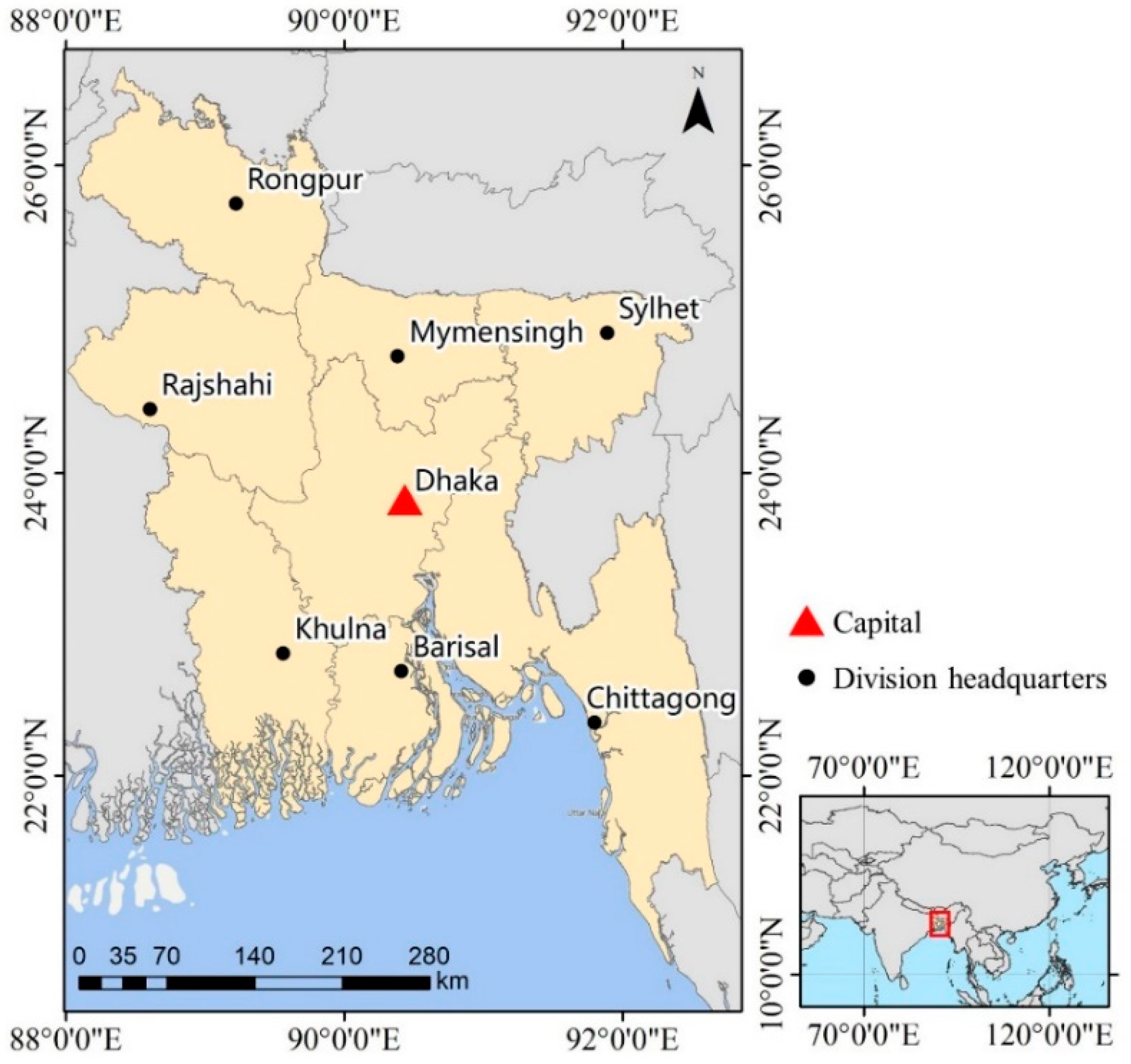
Bangladesh is a South Asian country consisting of eight administrative divisions, with Dhaka being its capital and the largest city (Figure 1). It is one of the most densely populated countries in the world with a sizable population still living in poverty. In 2014, the population and GDP in Bangladesh were $0.16 billion and $173 billion (USD), respectively [40]. It was a lower-middle income country at the time, according to the World Bank’s classification of countries by income. The poverty headcount ratio at national poverty lines (percentage of the population) was 31.5% in 2010 and 24.3% in 2016 [40]. In addition, Bangladesh possesses a highly complex and challenging physical environment, encountering yearly natural disasters such as floods, droughts and cyclone surges [41]. When faced with natural disasters, poor people are more likely to get injured or sick, but harder to recover [42]. Due to this, targeting the poverty in Bangladesh is important for both understanding the situation of poor people and developing policies to help them.
2.2. Data
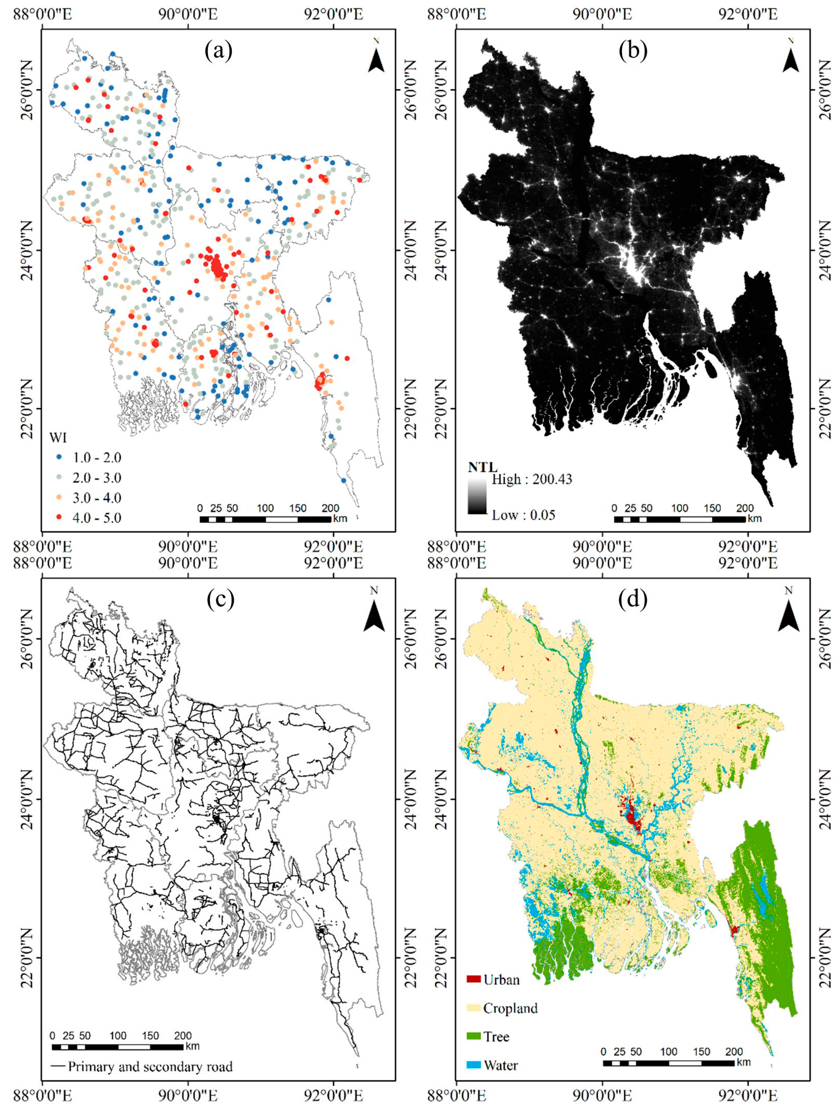
The Wealth Index (WI) (Figure 2a) drawn from the Demographic and Health Surveys (DHS) program [43,44,45] was used as the dependent variable of the poverty estimation model. WI is computed as the first principal component of household’s ownership of selected assets (such as televisions and bicycles, materials used for housing construction, types of water access and sanitation facilities) and has been used as a reflection of household poverty level in previous studies [28,30,46]. The WI value is an integer ranging from 1 to 5, indicating the lowest, second, middle, fourth, and the highest asset levels. The DHS provides WI for each household participating in the survey. Instead of specific household locations this dataset provides the average latitude and longitude of the groupings of households, known as household clusters. To further preserve the anonymity of survey respondents, the data collection agency displaced the positions of clusters by adding up to 5 km positional errors in each direction (1% of rural clusters contain up to 10 km positional error). We averaged the WI across households within the cluster to get the average WI of each cluster. In this study, the latest WI data in 2014 was used to represent the poverty level in Bangladesh. The final WI data consist of 598 household clusters, each of which contains between 3 to 30 households. The average and median number of households in each cluster were 28.8 and 29.
The VIIRS Cloud Mask–Outlier Removed (vcm–orm) annual composite NPP-VIIRS DNB data (Figure 2b) collected from the National Oceanic and Atmospheric Administration’s National Centers for Environmental Information (NOAA/NCEI) of the United States [47] were used to reflect the NTL intensity in Bangladesh. The annual composite NTL data were calculated as the average radiance values of the daily DNB data that had undergone stray light correction, lunar irradiance correction, cloud removal, and outlier removal procedure. The resolution of the data is 15 arc-second (~500 m). As the annual composite NTL data in 2015 and 2016 are the only available data, we chose the data in 2015 to minimize the temporal differences between the WI data, NTL data and the Google satellite images.
Google provides high resolution satellite images of cities around the world. In this study, Google satellite images were used to extract the structure and texture features of the landscape. We downloaded the Google satellite images at zoom level 16 with the size of each image being 224 × 224 pixels using the Google Static Maps API [48]. The spatial resolution of the image was ~2.39 m which is high enough to reflect the detailed landscape. The size of each image is ~535 m × 535 m (calculated as 224 × 2.39 m), which is similar in size to the NPP-VIIRS NTL pixel size. The dates of most Google images we used were from 2015 to 2017, which we downloaded in January 2018. The dates were close to WI data and other environmental data used in this study.
Maps illustrating the primary and secondary roads (Figure 2c) acquired from Open Street Map (OSM) [49] were used to calculate the accessibility of the region. Land cover maps at a 300-m resolution for 2015, acquired from the European Space Agency (ESA) Climate Change Initiative (CCI) project [50], were used to extract urban area as well as other land cover features. We integrated land cover types into four categories: urban, cropland, tree, and water (Figure 2d). The Administrative boundary and division headquarter data (Figure 1) were obtained from a geo-spatial data storing and sharing website provided by Bangladesh government [51].
2.3. Methods
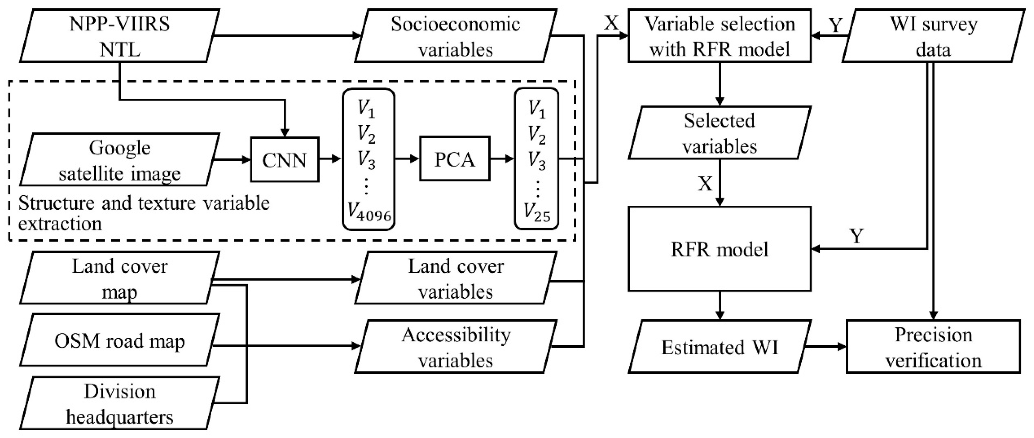
A flowchart of the RFR model to estimate WI is illustrated in Figure 3. We first extracted various features from multiple data sources described above and used these features as independent variables to develop and train a RFR model; these features were used to estimate the WI as the dependent variable in the model. Given that there is up to 5 km of positional error added for each WI cluster location, we generated a 10 km × 10 km grid centered at each cluster location to ensure that the true location falls within the grid. The 10 km × 10 km grid was then used as the basic unit of analysis and features were extracted for each grid.
2.3.1. Feature Extraction
We extracted four types of variables from multiple data sources. Table 1 lists the descriptions of all variables we used and the data source used to define and quantify the variables. Socioeconomic variables included three indices derived from NTL data (Mean, Min, and Max NTL). We used NTL indices to reflect socioeconomic conditions because NTL has proven to be correlated with many socioeconomic indicators [5,52,53]. Generally, the lower NTL intensity indicates less developed economy and high probability to be poor.
The physical living environment of households was reflected by structure and texture variables as well as land cover variables. Structure and texture variables were abstract variables that can reflect the detailed landscape feature such as the presence/absence of buildings, roads, and water [28], which are useful to quantify the detailed living environment. The structure and texture variables (PC1~PC25) were extracted from Google satellite images combined with NTL data by adapting a transfer learning model introduced by Jean et al. [28]. The procedures we took to extract structure and texture variables are described as follows.
Firstly, by fitting a Gaussian mixture model to the relative frequencies of the NTL intensity values across Bangladesh, the NTL values were classified into three classes, with the classes ranging from 0.0–0.65, 0.65–2.55, 2.55–200.43 , indicating low, medium, and high NTL intensity, respectively. Secondly, we fine-tuned a convolutional neural network (CNN) model named VGG-F [54] to predict NTL classes from the corresponding Google satellite images. Since NTL can reflect economic activities, the features that explain variation in NTL intensity is also predictive of economic outcomes such as poverty [28], which serves as a basis for the transfer learning method. The fine-tuned CNN model was then used as a feature extractor to extract these features. Thirdly, as the dimension of features extracted from the CNN model was large (4096-dimensions), we used the principal component analysis (PCA) to reduce the vector dimension to prevent overfitting to the relatively small training sets. The first 25 principal components retained 90% of data variation and were used in the following RFR model. Because each 10 km × 10 km grid covered 400 NTL and Google images, we got 400 feature vectors from each grid. We then averaged these feature vectors to obtain one feature vector for each grid.
Land cover variables described the composition of the surface landscape in terms of the amount of basic land cover types (including urban, cropland, tree, and water), which could reflect the overall living environment of the area. Land cover variables were computed as the proportion of each land cover type in each grid.
Accessibility features describe the convenience of households to access roads, urban, and division headquarters. Communities in remote locations away from roads and developed regions often have a large concentration of poverty because people in these communities often have poor access to infrastructure such as education, health facilities, transportation and participate in the market economy [31]. Accessibility features were computed as the distance from the grid center to roads, urban area, and division headquarters as well as the total road length in a grid. The urban areas were extracted from the land cover map (Figure 2d).
2.3.2. The RFR Model
RFR is a combination model that consists of a large number of regression trees. A regression tree [55] is defined as a flowchart-like structure in which the input dataset is repeatedly split into increasingly homogeneous subsets at each node and ends with a series of terminal nodes. Once a regression tree is trained using the training data, the predictions for new observations are determined by sending the input variables down the tree and taking the means of the response variables within the terminal node into which the observation fall [56]. In a RFR, each regression tree is constructed using a subset of training samples that is independently selected, with replacement from the original data set [32]. For each node per tree, only a small subset of variables is randomly selected to determine the split. This strategy increases the diversity between trees to avoid over-fitting and increases the robustness of the model. The final RFR predictor is formed by taking the average over all trees. The samples that are not used to grow the tree are called Out-Of-Bag (OOB) data. To estimate the model accuracy, the RFR gives an error of estimate called the OOB error by calculating the difference in the mean square errors between the OOB data and the data used to grow the regression trees [32]. To assess the explanatory power of each variable, Gini importance was used. Gini importance is defined as the total decrease in node impurity (weighted by the probability of reaching that node) averaged over all trees [57] and can be used as a general indicator of feature relevance. The sum of the Gini importance of all variables is 1.0. A higher Gini importance value indicates that the variable is relatively more important.
In our study, we implemented RFR by using a Python package named scikit-learn [58]. Firstly, we standardized the input variables, that is, features extracted from multiple data sources, by removing the mean and scaling to unit variance. Secondly, we used backward elimination method [59] to select variables that would offer the best predictive ability of the RFR model. We started the RFR model with all the variables and removed the least important variable at each iteration. If the OOB error of the model increased, we added this variable back to the model. We repeated this until no further improvement was observed on removal of variables. After that, we used the remaining variables to train the RFR model. When training the model, several parameters need to be determined. Table 2 shows the parameters that we optimized in the RFR model. The values of parameters were determined by the grid search method [60] using all the samples as the training data.
We estimated the WI values for 598 household clusters using a 10-fold cross validation approach, that is, the household clusters were randomly partitioned into 10 equal sized subsamples among which the WI values for each subsample were estimated using the model that was trained using the other nine subsamples. The R2 between the actual and estimated WI was used to evaluate the model performance. Once validated, the resulting RFR model was applied to the entire Bangladesh to obtain an estimate of the WI at 10 km × 10 km resolution.
2.3.3. Collinearity Analysis of Variables
To measure the collinearity between the variables used in the RFR model, we first calculated the Pearson correlation coefficient r between any two variables (except between any two principal components extracted from the Google satellite imagery given that the PCA ensures no correlation between principal components). Then, we calculated two indicators—tolerance and Variance Inflation Factor (VIF)—to further check the multicollinearity between variables:
where is the coefficient of determination of a regression of explanatory variable j on all the other explanators. A tolerance of less than 0.2 or a VIF of 5 and above indicates the existence of a multicollinearity problem [61].
3. Results
3.1. Variables Selection Results
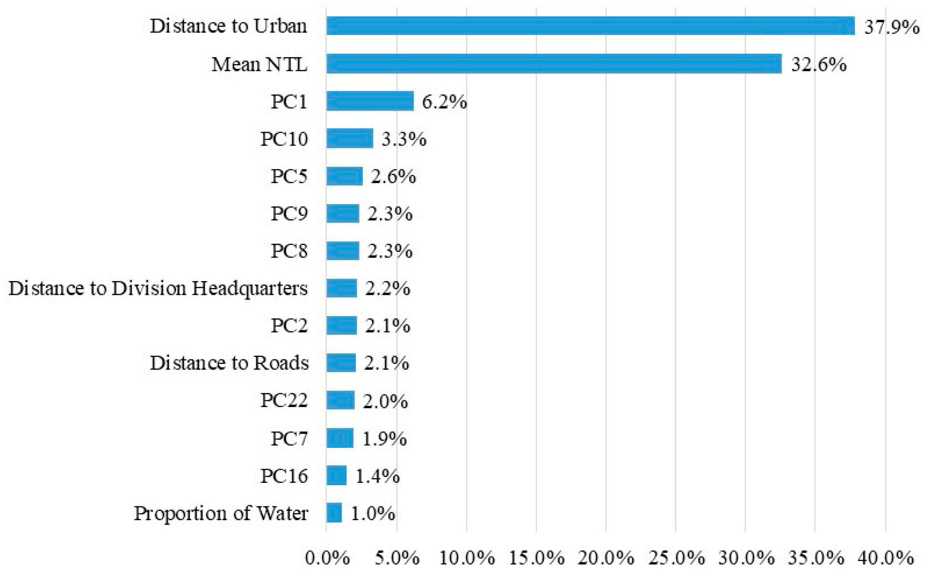
Selected variables ordered by Gini importance are shown in Figure 4. It shows that 14 out of the 36 variables were selected, with distance to urban being the most important variable with an importance weight of 37.9%. Amongst the four types of variable sets, accessibility variables (including distance to urban, distance to roads, and distance to division headquarters) were the most important variables with a total importance weight of 42.2%, indicating that accessibility was the key factor to estimate poverty level. On the other hand, 9 out of the 25 structure and texture variables extract from Google satellite images were selected (including PC1, PC10, PC5, PC8, PC9, PC2, PC7, PC22, and PC16) with a collective importance weightage of 24.1%. The mean NTL was the only socioeconomic variable that was retained with an importance weight of 32.6%, whereas the proportion of water was the only land cover variable that was retained with a marginal importance weight of 1.0%.
3.2. Accuracy Evaluation of the RFR Model
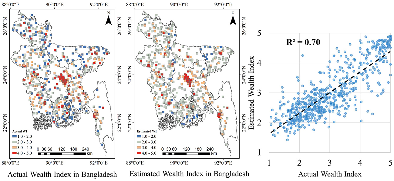
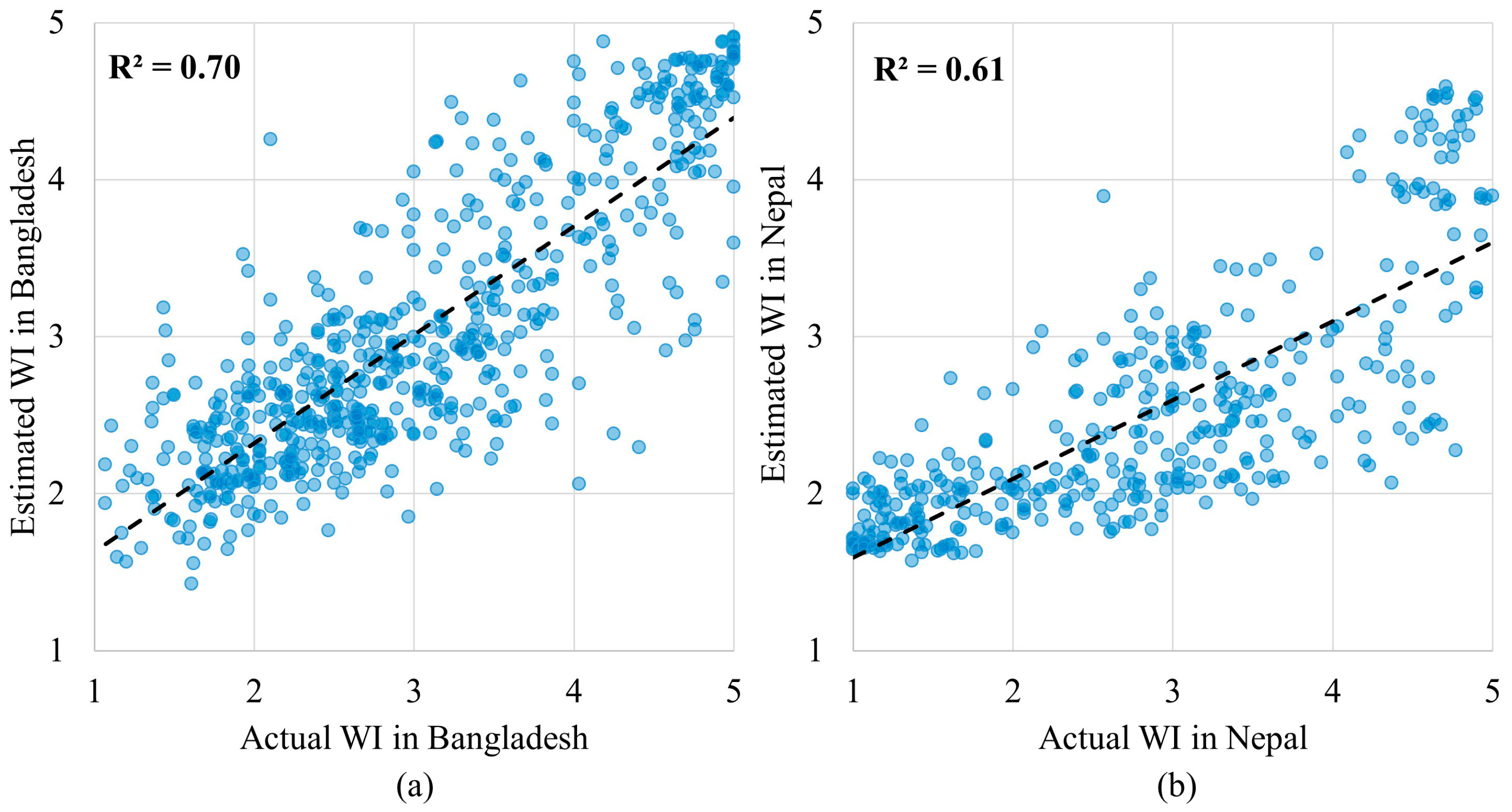
To evaluate the accuracy of the proposed RFR model, we calculated the R2 between the actual and estimated WI in Bangladesh (Figure 5a). The R2 of 0.70 indicates a strong correlation between the actual and estimated WI, showing a good performance of the RFR model. To test whether the model trained using data from Bangladesh could be used to estimate the poverty in other countries, we applied the model to estimate the WI in Nepal by using variables extracted from multiple data sources in Nepal as model inputs. We chose Nepal because it is geographically close to Bangladesh and is a low-income country according to the World Bank’s classification of countries by income. More importantly, the DHS provided WI data for Nepal in 2016, which can be used to validate the model results. We compared the estimated WI with the actual WI in Nepal (Figure 5b). The R2 of 0.61 indicates a good generalization ability of our model.
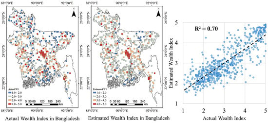
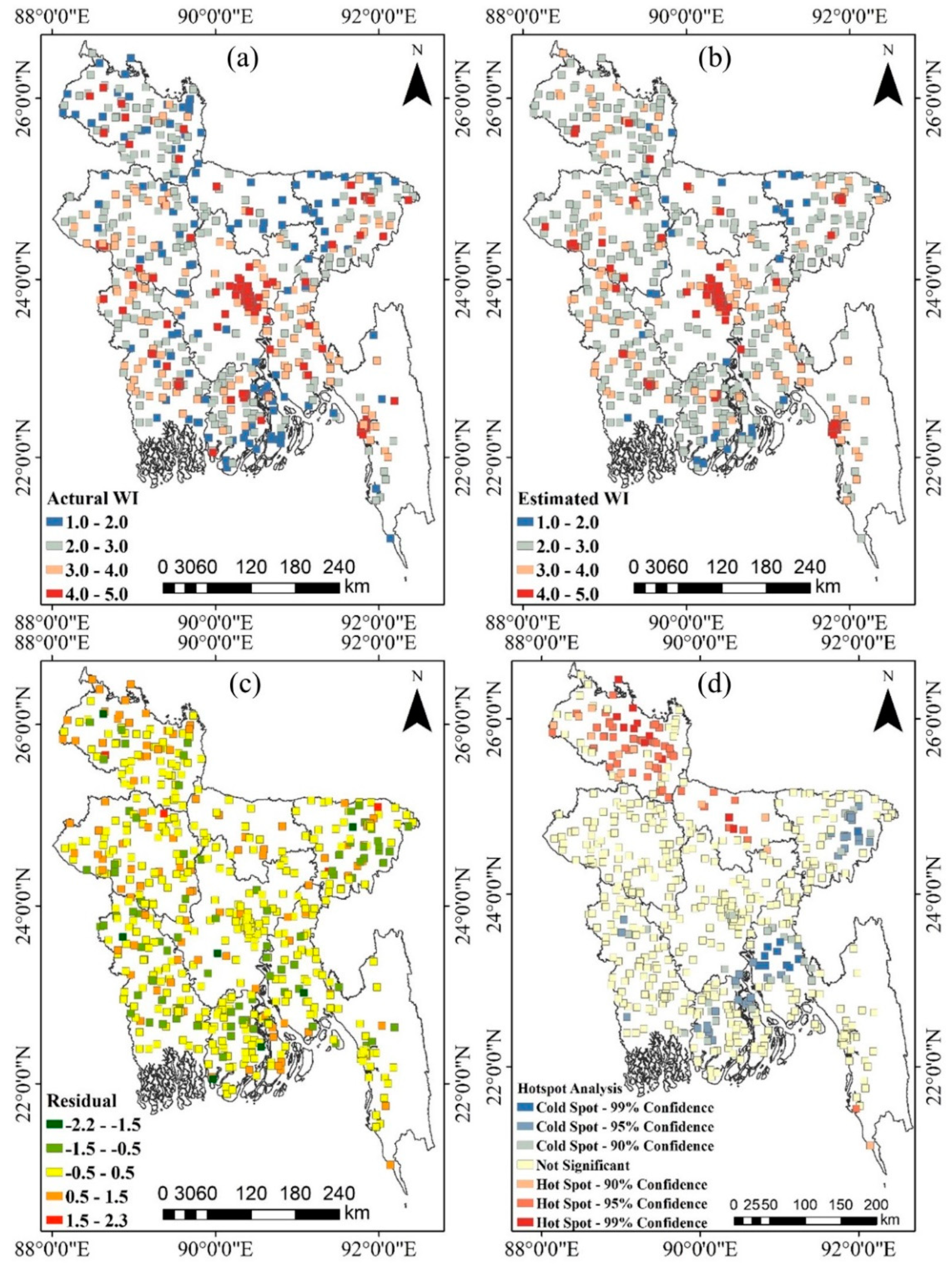
Figure 6a,b presents the spatial distribution of the actual and estimated WI in Bangladesh, respectively. The actual and the estimated WI distribute very similar patterns geographically across Bangladesh. However, the range of the estimated WI (from 1.43 to 4.91) was smaller than that of the actual WI (from 1.07 to 5.0), indicating that the proposed method has compressed the data range to some extent. Figure 6c shows the residuals between the actual and the estimated WI, calculated as the estimated WI minus the actual WI. Most of the residuals fall within the −0.5 to 0.5 range (represented in yellow color in Figure 6c), indicating an overall small difference between the actual and estimated WI. In order to further analyze the spatial distribution of residuals, we conducted a hotspot analysis of the residuals using the Getis–Ord (Gi*) statistic [62]. The result showed that the cold spots were mainly distributed in places with high WI values, while the hot spots were mainly distributed in places with low WI value (Figure 6d), indicating that the proposed method tends to underestimate the high WI values and overestimate the low WI values.
3.3. Accuracy Evaluation by A Comparison with District-Level Census Data
Using the RFR model, we reconstructed the 10 km × 10 km poverty map for the whole of Bangladesh (Figure 7a). Areas where the model assigns a low WI were colored blue, while areas assigned a high WI were colored red. We aggregated the estimated WI to the district level by calculating the average WI value of all grids in each district (Figure 7b). As a validity check, we compared the aggregated WI against the most recent poverty Head Count Rate (HCR) map (Figure 7c), which was derived based on the 2015 survey data [63]. Both the WI map and poverty HCR map were classified into five grades using the Jenks natural breaks [64] classification method. The patterns shown in these two maps are largely similar.
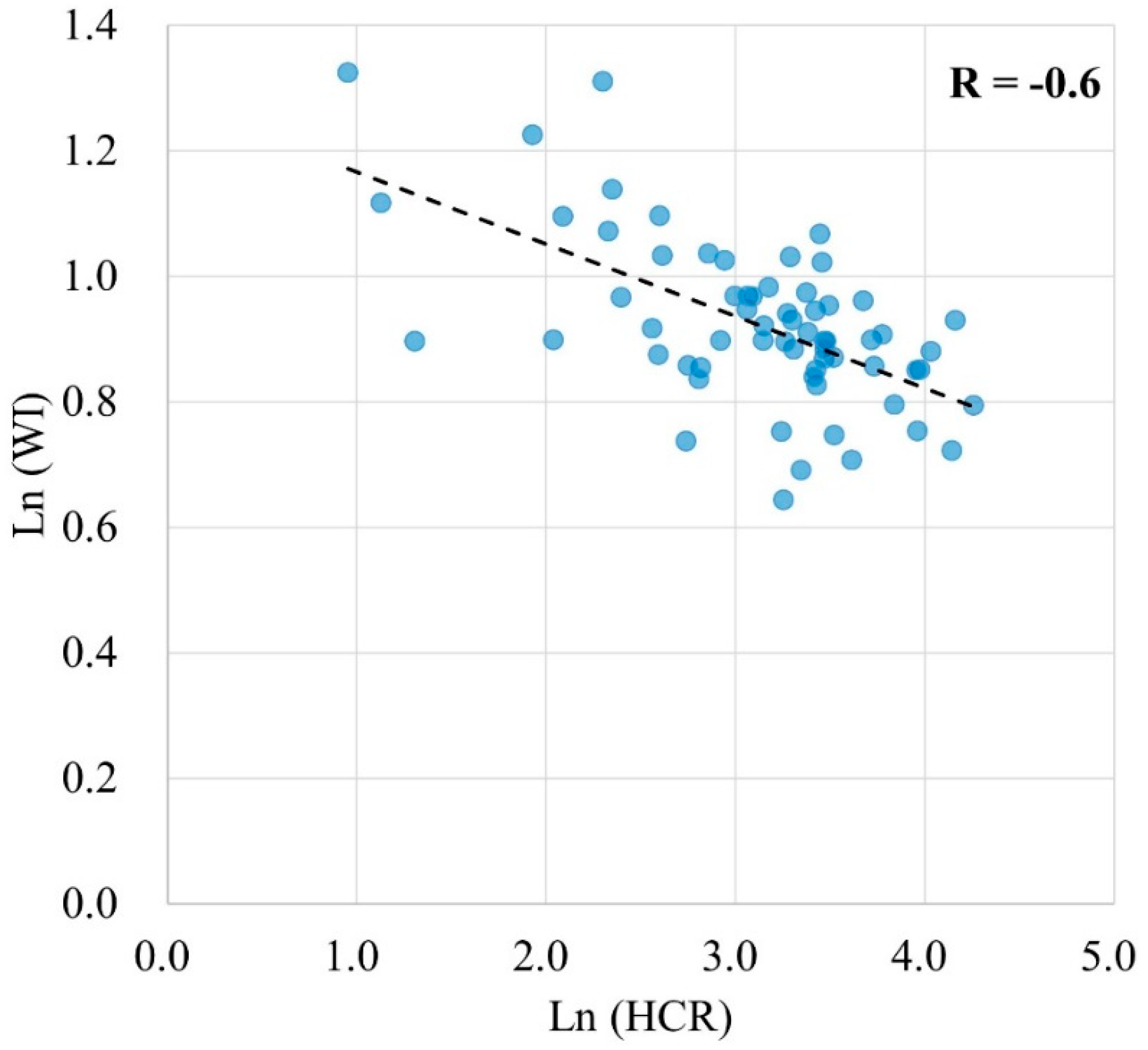
Furthermore, we calculated the Pearson correlation coefficient (r) between the log-transformed poverty HCR and estimated WI. The log transformation was applied to decrease the variability of data and make the data conform more closely to a normal distribution. The r of −0.60 (p < 0.001) indicates a negative correlation between the log-scaled poverty HCR and WI (Figure 8).
3.4. Collinearity of Variables
Table 3 lists the Pearson correlation coefficient r between any two variables used in the RFR model (except between any two principal components extracted from Google satellite image). There was a strong correlation between the mean NTL and PC1 (r = 0.90). Apart from this set of variables, the r values between any other pair of variables were less than 0.50, indicating no strong correlation between them.
Table 4 lists the tolerance and VIF of all variables used in the RFR model. The tolerance of mean NTL and PC1 were both under 0.2, and the VIF larger than 5, indicating the existence of the multicollinearity problem. However, both of them were indispensable since discarding either of them would result in a substantial decrease in the accuracy of the model.
4. Discussion
This study applies a RFR model for estimating poverty at 10 km × 10 km spatial resolution using variables extracted from multiple data sources in Bangladesh. The R2 between the estimated WI from 10-fold cross validation and the actual WI in Bangladesh is 0.70, which is relatively high compared to the results in previous research [23,25,27,28]. By applying the model trained in Bangladesh to Nepal, we tested the replicability of the model in different geographical context. The R2 between the estimated and actual WI of 0.61 in Nepal indicated a relatively good generalization ability compared to the previous research [28], which used a model trained in one country to estimate WI in other five countries with R2 between estimated and actual WI ranging from 0.24 to 0.71. Our results show that a relatively accurate estimation can be made by using multiple environmental data sources. Therefore, for countries that lack survey data, the RFR model can be used by using training data in other countries to estimate poverty.
The overall small residuals indicate a relatively accurate predictive power of our model. However, the results of the residual analysis also indicate that the proposed RFR model tends to underestimate high WI values and overestimate low WI values. That is because the final result of a RFR model is the average result over all the trees that formed the RFR. Therefore, it is impossible to predict either beyond the range of response values in the training data, or within the entire range of the response values [65]. That would result in the underestimation of high values and overestimation of low values. This is an inherent limitation of the RFR model. When we aggregate the data to the district-level, and valid the model results with the HCR data, a negative correlation between the average WI and the poverty HCR was established, which is in line with our perception that poor areas tend to have lower average household assets and a higher proportion of poor people. The correlation between them was not very high (r = −0.60) due to the different measuring methods. WI was calculated based on household’s ownership of several assets as a reflection of wealth, whereas poverty HCR was computed as the proportion of poor people in each division. Despite this difference, it still shows that the aggregated WI can partially reflect the district-level poverty HCR.
To test whether our RFR model improves upon the direct use of Google satellite images or NTL to estimate WI, we compared the results from our RFR model with the outcome from two other models. The first was a transfer learning model that used the 4096-dimensional feature vector from the Google satellite images along with the WI data to train a ridge regression model to estimate the WI [28]. The second model used a linear regression to estimate the WI from the log-transformed NTL data [65]. We also compared our results with a RFR model that excludes variables extracted from Google satellite images. This comparison was practiced to assess the extent the model without Google satellite images can estimate WI given that time-consuming nature for computing the Google image data. Table 5 shows the R2 between the estimated and actual WI from all four methods.
The R2 of the linear regression model using the log-transformed NTL was 0.58, which was lower than the R2 of our proposed RFR model. The R2 of the transfer learning model was 0.63. Previous research [28] using the same method got the R2 values of 0.55, 0.58, 0.66, 0.69, and 0.75 for five countries in Africa. Our result was within this range, indicating that the transfer learning model can be applied to Bangladesh and our estimation was reasonable. Compared to models that used NTL and Google satellite imagery in isolation to estimate poverty, our RFR model had a higher accuracy. This proves that our RFR model can increase the poverty estimation accuracy by adding different types of data. The R2 of the RFR model that excludes features extracted from Google satellite images was 0.66, which was slightly lower than the proposed RFR model and higher than the transfer learning model that used Google satellite images only. Considering the time-consuming nature of computing the Google image data, the RFR-based model without using Google satellite images was more efficient and accurate than the transfer learning model.
The analysis of the variables’ importance shows that accessibility variables were the most import variables to estimate poverty, indicating that the variations in distance to roads, urban and division headquarters are most likely to lead to variations in poverty level. This also illustrates that communities in regions that are far from roads, urban and large cities tend to have limited resources and are therefore more inclined to poverty. Socioeconomic variables can directly reflect the economic condition and were assessed to be the second important variables. Amongst the three socioeconomic variables, minimum NTL and maximum NTL radiance were discarded because their variations can be expressed by the variation of the mean NTL. Amongst the land cover variables, the proportion of urban, cropland, and tree were discarded probably because the features extracted from Google satellite images can reflect more detailed land cover information by providing the spatial distribution of each type of land cover rather than the proportion.
The collinearity analysis of the variables shows that there is strong collinearity between PC1 and mean NTL. Besides, the correlation between some other variables, although not strong, was statistically significant. Despite this, the RFR model still has good ability to estimate poverty. The analysis of the importance of variables shows that all of these variables contribute to the RFR model. In addition, discarding either of them would result in a decrease in accuracy of the model, indicating that the differences between them still contribute to the RFR model. This shows that RFR model has the ability to handle multicollinearity because the variables used to train each tree in a RFR model are different given that each of them were selected randomly from all variables. Therefore, the RFR model is not constrained to selecting only independent variables to estimate poverty.
5. Conclusions
There is pressing need to identify reliable data for poverty estimation in the absence of poverty survey data. While remote sensing data and road maps can reflect some of the environmental characteristics that are associated with poverty, existing studies are limited in using such data in isolation rather than collectively to represent the multidimensional construct of poverty and improve the accuracy of estimation. This study explores an integration of multi-source data and a RFR model to estimate poverty at 10 km × 10 km resolution. The WI for household clusters was used as the dependent variable to reflect poverty level and model training was conducted in Bangladesh. Thirty-six independent variables representing four poverty dimensions including socioeconomic status, structure and texture, land cover, and accessibility were extracted from NPP-VIIRS NTL data, Google satellite imagery, land cover map, OSM road map, and the division headquarter map. Following a vigorous variable selection procedure, 14 variables that offered the best predictive ability of the RFR model were reserved to train the final RFR model. After training the RFR model, we verified the accuracy of the model in three ways. Firstly, we calculated the R2 between the actual WI and the WI estimated from 10-fold cross validation in Bangladesh. A high overall accuracy of our RFR model with an R2 of 0.70 was obtained to estimate poverty at 10 km × 10 km resolution. Analysis of the residuals shows that the RFR model tends to underestimate the high WI values and overestimate the low WI values. Secondly, the trained RFR model was applied to Nepal to test whether the model trained in one country can be used to estimate poverty in another country. The R2 between the actual and estimated WI in Nepal was 0.61, indicating a good generalization ability of our model. Thirdly, we calculated the average WI of each district and compared it to the district level poverty HCR. The r of −0.60 showed a relatively strong negative correlation between them, indicating that the results of our RFR model can reflect poverty HCR at the district level to some extent. Gini importance was used to assess the explanatory power of each variable. Accessibility variables were the most important variables to estimate WI with the total importance of 42.2%, followed by socioeconomic variables (32.6%), structure and texture variables (24.1%), and land cover variables (1.0%). Although there was multicollinearity between variables, the proposed RFR had good ability to estimate poverty, which confirmed the finding that the RFR model has the ability to handle multicollinearity [35,38]. Compared to other methods that used NTL or Google satellite imagery in isolation to estimate poverty, our method has produced higher accuracy by using multi-source data. All data we use in this study, including NPP-VIIRS NTL data, Google satellite imagery, land cover data, OSM road map, and division headquarter location map, are publicly and globally available. Therefore, the proposed model can be easily applied to other countries or regions.
This study has some limitations. Firstly, the acquisition time of the data in use was different. The WI survey data were obtained in 2014, while the NTL and land cover data were obtained in 2015, the road map was in 2018 and Google satellite data were from 2015 to 2017. As the Bangladesh government has been working to eradicate poverty, the poverty level could be changing every year. Therefore, differences in data acquisition time could result in reduced estimation accuracy. Secondly, the location of the WI data was not accurate due to the up to 5 km of positional errors added by the data collection agencies to protect the privacy of survey respondents, which could also contribute to noise in the model accuracy assessment. Furthermore, given the 5-km positional error, we estimated WI at 10-km resolution, which was relatively rough. Further training and validation of the estimation can be achieved and higher resolution estimation can be conducted as more environmental data and more accurate poverty survey data become available.
Author Contributions
Conceptualization, B.Y., Y.L., X.Z. and J.W.; methodology, X.Z., B.Y., Y.L. and Z.C.; software, X.Z., Z.C., Q.L. and C.W.; formal analysis, X.Z., B.Y., Y.L., Z.C., Q.L. and C.W.; writing—original draft preparation, X.Z.; writing—review and editing, Y.L. and B.Y.; supervision, B.Y., Y.L. and J.W.; funding acquisition, B.Y., Y.L., Z.C. and X.Z.
Funding
This research was funded by the National Natural Science Foundation of China (No. 41871331 and 41801343), the Australian Research Council Discovery Project (DP170104235) and the China Scholarship Council (No. 201706140143) for Xizhi Zhao to conduct the research on which this paper is based at the University of Queensland.
Acknowledgments
The authors would like to thank the editor and two anonymous reviewers for their constructive comments on an earlier version of this paper.
Conflicts of Interest
The authors declare no conflicts of interest.
References
- United Nations. About the Sustainable Development Goals. Available online: https://www.un.org/sustainabledevelopment/sustainable-development-goals/ (accessed on 31 January 2019).
- Decline of Global Extreme Poverty Continues but Has Slowed: World Bank. Available online: http://www.worldbank.org/en/news/press-release/2018/09/19/decline-of-global-extreme-poverty-continues-but-has-slowed-world-bank (accessed on 15 December 2018).
- Coudouel, A.; Hentschel, J.S.; Wodon, Q.T. Poverty measurement and analysis. In A Sourcebook for Poverty Reduction Strategies; Klugman, J., Ed.; World Bank: Washington, DC, USA, 2002; Volume 1, pp. 27–74. [Google Scholar]
- Carvalho, S.; White, H. Combining the Quantitative and Qualitative Approaches to Poverty Measurement and Analysis: The Practice and the Potential; World Bank technical paper; no. WTP 366; The World Bank: Washington, DC, USA, 1997. [Google Scholar]
- Shi, K.; Yu, B.; Huang, Y.; Hu, Y.; Yin, B.; Chen, Z.; Chen, L.; Wu, J. Evaluating the Ability of NPP-VIIRS Nighttime Light Data to Estimate the Gross Domestic Product and the Electric Power Consumption of China at Multiple Scales: A Comparison with DMSP-OLS Data. Remote Sens. 2014, 6, 1705–1724. [Google Scholar] [CrossRef] [Green Version]
- Zhao, N.; Liu, Y.; Cao, G.; Samson, E.L.; Zhang, J. Forecasting China’s GDP at the pixel level using nighttime lights time series and population images. GISci. Remote Sens. 2017, 54, 407–425. [Google Scholar] [CrossRef]
- Sutton, P.; Roberts, D.; Elvidge, C.; Baugh, K. Census from Heaven: An estimate of the global human population using night-time satellite imagery. Int. J. Remote Sens. 2001, 22, 3061–3076. [Google Scholar] [CrossRef]
- Sutton, P.; Roberts, C.; Elvidge, C.; Meij, H. A comparison of nighttime satellite imagery and population density for the continental united states. Photogramm. Eng. Remote Sens. 1997, 63, 1303–1313. [Google Scholar]
- Chand, T.K.; Badarinath, K.; Elvidge, C.; Tuttle, B. Spatial characterization of electrical power consumption patterns over India using temporal DMSP-OLS night-time satellite data. Int. J. Remote Sens. 2009, 30, 647–661. [Google Scholar] [CrossRef]
- Shi, K.; Yu, B.; Huang, C.; Wu, J.; Sun, X. Exploring spatiotemporal patterns of electric power consumption in countries along the Belt and Road. Energy 2018, 150, 847–859. [Google Scholar] [CrossRef]
- Shi, K.; Chen, Y.; Yu, B.; Xu, T.; Yang, C.; Li, L.; Huang, C.; Chen, Z.; Liu, R.; Wu, J. Detecting spatiotemporal dynamics of global electric power consumption using DMSP-OLS nighttime stable light data. Appl. Energy 2016, 184, 450–463. [Google Scholar] [CrossRef]
- Shi, K.; Yang, Q.; Fang, G.; Yu, B.; Chen, Z.; Yang, C.; Wu, J. Evaluating spatiotemporal patterns of urban electricity consumption within different spatial boundaries: A case study of Chongqing, China. Energy 2019, 167, 641–653. [Google Scholar] [CrossRef]
- Shi, K.; Chen, Y.; Yu, B.; Xu, T.; Chen, Z.; Liu, R.; Li, L.; Wu, J. Modeling spatiotemporal CO2 (carbon dioxide) emission dynamics in China from DMSP-OLS nighttime stable light data using panel data analysis. Appl. Energy 2016, 168, 523–533. [Google Scholar] [CrossRef]
- Ghosh, T.; Elvidge, C.D.; Sutton, P.C.; Baugh, K.E.; Ziskin, D.; Tuttle, B.T. Creating a global grid of distributed fossil fuel CO2 emissions from nighttime satellite imagery. Energies 2010, 3, 1895–1913. [Google Scholar] [CrossRef]
- Chen, Z.Q.; Yu, B.L.; Hu, Y.J.; Huang, C.; Shi, K.F.; Wu, J.P. Estimating House Vacancy Rate in Metropolitan Areas Using NPP-VIIRS Nighttime Light Composite Data. IEEE J. Sel. Top. Appl. Earth Obs. Remote Sens. 2015, 8, 2188–2197. [Google Scholar] [CrossRef]
- Shi, K.; Yu, B.; Hu, Y.; Huang, C.; Chen, Y.; Huang, Y.; Chen, Z.; Wu, J. Modeling and mapping total freight traffic in China using NPP-VIIRS nighttime light composite data. GISci. Remote Sens. 2015, 52, 274–289. [Google Scholar] [CrossRef]
- Yu, B.; Shu, S.; Liu, H.; Song, W.; Wu, J.; Wang, L.; Chen, Z. Object-based spatial cluster analysis of urban landscape pattern using nighttime light satellite images: a case study of China. Int. J. Geogr. Inf. Sci. 2014, 28, 2328–2355. [Google Scholar] [CrossRef]
- Shi, K.; Huang, C.; Yu, B.; Yin, B.; Huang, Y.; Wu, J. Evaluation of NPP-VIIRS nighttime light composite data for extracting built-up urban areas. Remote Sens. Lett. 2014, 5, 358–366. [Google Scholar] [CrossRef]
- Chen, Z.; Yu, B.; Song, W.; Liu, H.; Wu, Q.; Shi, K.; Wu, J. A New Approach for Detecting Urban Centers and Their Spatial Structure With Nighttime Light Remote Sensing. IEEE Trans. Geosci. Remote Sens. 2017, 55, 6305–6319. [Google Scholar] [CrossRef]
- Yu, B.; Tang, M.; Wu, Q.; Yang, C.; Deng, S.; Shi, K.; Peng, C.; Wu, J.; Chen, Z. Urban Built-Up Area Extraction From Log-Transformed NPP-VIIRS Nighttime Light Composite Data. IEEE Geosci. Remote Sens. Lett. 2018. [Google Scholar] [CrossRef]
- Elvidge, C.D.; Cinzano, P.; Pettit, D.; Arvesen, J.; Sutton, P.; Small, C.; Nemani, R.; Longcore, T.; Rich, C.; Safran, J. The Nightsat mission concept. Int. J. Remote Sens. 2007, 28, 2645–2670. [Google Scholar] [CrossRef]
- Elvidge, C.D.; Baugh, K.; Zhizhin, M.; Hsu, F.C.; Ghosh, T. VIIRS night-time lights. Int. J. Remote Sens. 2017, 38, 5860–5879. [Google Scholar] [CrossRef] [Green Version]
- Noor, A.M.; Alegana, V.A.; Gething, P.W.; Tatem, A.J.; Snow, R.W. Using remotely sensed night-time light as a proxy for poverty in Africa. Popul. Health Metr. 2008, 6, 5. [Google Scholar] [CrossRef] [PubMed] [Green Version]
- Elvidge, C.D.; Sutton, P.C.; Ghosh, T.; Tuttle, B.T.; Baugh, K.E.; Bhaduri, B.; Bright, E. A global poverty map derived from satellite data. Comput. Geosci. 2009, 35, 1652–1660. [Google Scholar] [CrossRef]
- Yu, B.; Shi, K.; Hu, Y.; Huang, C.; Chen, Z.; Wu, J. Poverty Evaluation Using NPP-VIIRS Nighttime Light Composite Data at the County Level in China. IEEE J. Sel. Top. Appl. Earth Obs. Remote Sens. 2015, PP, 1–13. [Google Scholar] [CrossRef]
- Varshney, K.R.; Chen, G.H.; Abelson, B.; Nowocin, K.; Sakhrani, V.; Xu, L.; Spatocco, B.L. Targeting Villages for Rural Development Using Satellite Image Analysis. Big Data 2015, 3, 41–53. [Google Scholar] [CrossRef] [PubMed]
- Duque, J.C.; Patino, J.E.; Ruiz, L.A.; Pardo-Pascual, J.E. Measuring intra-urban poverty using land cover and texture metrics derived from remote sensing data. Landsc. Urban Plann. 2015, 135, 11–21. [Google Scholar] [CrossRef] [Green Version]
- Jean, N.; Burke, M.; Xie, M.; Davis, W.M.; Lobell, D.B.; Ermon, S. Combining satellite imagery and machine learning to predict poverty. Science 2016, 353, 790–794. [Google Scholar] [CrossRef] [PubMed]
- Watmough, G.R.; Atkinson, P.M.; Hutton, C.W. Predicting socioeconomic conditions from satellite sensor data in rural developing countries: A case study using female literacy in Assam, India. Appl. Geogr. 2013, 44, 192–200. [Google Scholar] [CrossRef]
- Weiss, D.; Nelson, A.; Gibson, H.; Temperley, W.; Peedell, S.; Lieber, A.; Hancher, M.; Poyart, E.; Belchior, S.; Fullman, N. A global map of travel time to cities to assess inequalities in accessibility in 2015. Nature 2018, 553, 333. [Google Scholar] [CrossRef] [PubMed]
- Sen, B. Drivers of escape and descent: Changing household fortunes in rural Bangladesh. World Develop. 2003, 31, 513–534. [Google Scholar] [CrossRef]
- Breiman, L. Random forests. In Machine learning; Schapire, R.E., Ed.; Kluwer Academic Publishers: Boston, MA, USA, 2001; Volume 45, pp. 5–32. [Google Scholar]
- Abdel-Rahman, E.M.; Ahmed, F.B.; Ismail, R. Random forest regression and spectral band selection for estimating sugarcane leaf nitrogen concentration using EO-1 Hyperion hyperspectral data. Int. J. Remote Sens. 2012, 34, 712–728. [Google Scholar] [CrossRef]
- Immitzer, M.; Atzberger, C.; Koukal, T. Tree Species Classification with Random Forest Using Very High Spatial Resolution 8-Band WorldView-2 Satellite Data. Remote Sens. 2012, 4, 2661–2693. [Google Scholar] [CrossRef] [Green Version]
- Wang, L.a.; Zhou, X.; Zhu, X.; Dong, Z.; Guo, W. Estimation of biomass in wheat using random forest regression algorithm and remote sensing data. The Crop Journal 2016, 4, 212–219. [Google Scholar] [CrossRef] [Green Version]
- Stevens, F.R.; Gaughan, A.E.; Linard, C.; Tatem, A.J. Disaggregating census data for population mapping using random forests with remotely-sensed and ancillary data. PLoS ONE 2015, 10, e0107042. [Google Scholar] [CrossRef]
- Yao, Y.; Liu, X.; Li, X.; Zhang, J.; Liang, Z.; Mai, K.; Zhang, Y. Mapping fine-scale population distributions at the building level by integrating multisource geospatial big data. Int. J. Geogr. Inf. Sci. 2017. [Google Scholar] [CrossRef]
- Belgiu, M.; Drăguţ, L. Random forest in remote sensing: A review of applications and future directions. ISPRS J. Photogramm. Remote Sens. 2016, 114, 24–31. [Google Scholar] [CrossRef]
- Van Beijma, S.; Comber, A.; Lamb, A. Random forest classification of salt marsh vegetation habitats using quad-polarimetric airborne SAR, elevation and optical RS data. Remote Sens. Environ. 2014, 149, 118–129. [Google Scholar] [CrossRef]
- The World Bank Data—Bangladesh. Available online: https://data.worldbank.org/country/bangladesh (accessed on 31 October 2018).
- ADB. ADB Annual Report 2005; Asian Development Bank: Mandaluyong, Metro Manila, Philippines, 2005. [Google Scholar]
- Ahmed, S.A.; Diffenbaugh, N.S.; Hertel, T.W. Climate volatility deepens poverty vulnerability in developing countries. Environ. Res. Lett. 2009, 4, 8. [Google Scholar] [CrossRef]
- ICF. The DHS Program. Available online: https://dhsprogram.com/data/ (accessed on 31 October 2018).
- Rutstein, S.O. The DHS Wealth Index: Approaches for Rural and Urban Areas; Macro International: Calverton, MD, USA, 2008. [Google Scholar]
- ICF. Demographic and Health Surveys; Funded by USAID; ICF: Rockville, MD, USA, 2018. [Google Scholar]
- Smith, B.; Wills, S. Left in the dark? oil and rural poverty. J. Assoc. Environ. Resour. Econ. 2016, 5, 865–904. [Google Scholar] [CrossRef]
- Version 1 VIIRS Day/Night Band Nighttime Lights. Available online: https://ngdc.noaa.gov/eog/viirs/download_dnb_composites.html (accessed on 5 November 2018).
- Google Maps Platform-Maps Static API. Available online: https://developers.google.com/maps/documentation/maps-static/intro (accessed on 11 January 2018).
- Open Street Map. Available online: https://www.openstreetmap.org (accessed on 9 March 2018).
- European Space Agency Climate Change Initiatiue Land Cover. Available online: http://maps.elie.ucl.ac.be/CCI/viewer/ (accessed on 6 October 2018).
- GeoDASH. Available online: https://geodash.gov.bd/ (accessed on 11 March 2018).
- Ma, T.; Zhou, C.H.; Pei, T.; Haynie, S.; Fan, J.F. Responses of Suomi- NPP VIIRS- derived nighttime lights to socioeconomic activity in China’s cities. Remote Sens. Lett. 2014, 5, 165–174. [Google Scholar] [CrossRef]
- Zhou, Y.K.; Ma, T.; Zhou, C.H.; Xu, T. Nighttime Light Derived Assessment of Regional Inequality of Socioeconomic Development in China. Remote Sens. 2015, 7, 1242–1262. [Google Scholar] [CrossRef] [Green Version]
- Chatfield, K.; Simonyan, K.; Vedaldi, A.; Zisserman, A. Return of the devil in the details: Delving deep into convolutional nets. In Proceedings of the British Machine Vision Conference, Nottingham, UK, 1–5 September 2014. [Google Scholar]
- Venables, W.N.; Ripley, B.D. Tree-based methods. In Modern Applied Statistics with S; Springer: New York, NY, USA, 2002; pp. 251–269. [Google Scholar]
- Dasgupta, A.; Sun, Y.V.; König, I.R.; Bailey-Wilson, J.E.; Malley, J.D. Brief review of regression-based and machine learning methods in genetic epidemiology: the Genetic Analysis Workshop 17 experience. Genetic Epidemiology 2011, 35, S5–S11. [Google Scholar] [CrossRef] [Green Version]
- Breiman, L. Classification and Regression Trees; Routledge: New York, NY, USA, 1984. [Google Scholar] [CrossRef]
- Scikit-Learn. Available online: https://scikit-learn.org/stable/index.html (accessed on 10 December 2018).
- Guyon, I.; Elisseeff, A. An introduction to variable and feature selection. J. Mach. Learn. Res. 2003, 3, 1157–1182. [Google Scholar] [CrossRef]
- Lerman, P. Fitting segmented regression models by grid search. Appl. Stat. 1980, 77–84. [Google Scholar] [CrossRef]
- O’brien, R.M. A Caution Regarding Rules of Thumb for Variance Inflation Factors. Qual. Quant. 2007, 41, 673–690. [Google Scholar] [CrossRef]
- Getis, A.; Ord, J.K. The analysis of spatial association by use of distance statistics. Geogr. Anal. 1992, 24, 189–206. [Google Scholar] [CrossRef]
- Bangladesh Bureau of Statistics. Preliminary Report on Household Income and Expenditure Survey 2016; Bangladesh Bureau of Statistics: Dhaka, Bangladesh, October 2017.
- Brewer, C.A.; Pickle, L. Evaluation of methods for classifying epidemiological data on choropleth maps in series. Ann. Assoc. Am. Geogr. 2002, 92, 662–681. [Google Scholar] [CrossRef]
- Kühnlein, M.; Appelhans, T.; Thies, B.; Nauss, T. Improving the accuracy of rainfall rates from optical satellite sensors with machine learning—A random forests-based approach applied to MSG SEVIRI. Remote Sens. Environ. 2014, 141, 129–143. [Google Scholar] [CrossRef]
Figure 1.
Location of Bangladesh and its division headquarters.

Figure 2.
Datasets used in this study. (a) Wealth Index (WI) map, (b) National Polar-orbiting Partnership Visible Infrared Imaging Radiometer Suite (NPP-VIIRS) nighttime light (NTL) image, (c) Open Street Map (OSM) primary and secondary road map, (d) land cover map.
Figure 2.
Datasets used in this study. (a) Wealth Index (WI) map, (b) National Polar-orbiting Partnership Visible Infrared Imaging Radiometer Suite (NPP-VIIRS) nighttime light (NTL) image, (c) Open Street Map (OSM) primary and secondary road map, (d) land cover map.

Figure 3.
Flowchart to estimate WI with the proposed Random Forest Regression (RFR) model.

Figure 4.
The Gini importance of selected variables.

Figure 5.
Scatter plot between the actual WI and the estimated WI in (a) Bangladesh and (b) Nepal.

Figure 6.
The comparison between actual and estimated WI in Bangladesh. (a) Actual WI; (b) estimated WI; (c) residual between the actual and estimated WI; and (d) hotspot analysis of the residuals.
Figure 6.
The comparison between actual and estimated WI in Bangladesh. (a) Actual WI; (b) estimated WI; (c) residual between the actual and estimated WI; and (d) hotspot analysis of the residuals.

Figure 7.
The estimated WI at grid-level and district-level as well as the survey results for comparison. (a) The estimated WI at grid-level; (b) the estimated WI aggregated at the district-level; (c) Poverty Head Count Ratio (HCR) map.
Figure 7.
The estimated WI at grid-level and district-level as well as the survey results for comparison. (a) The estimated WI at grid-level; (b) the estimated WI aggregated at the district-level; (c) Poverty Head Count Ratio (HCR) map.

Figure 8.
Scatter plot between the log-scaled poverty HCR (x-axis) and the estimated WI (y-axis).


Table 1.
Independent variables derived from multi-source data.
| Variable Type | Variable Name | Description | Data Source |
|---|---|---|---|
| Socioeconomic | Mean NTL | The mean radiance value of NTL in each grid. | NPP-VIIRS NTL |
| Min NTL | The minimum radiance value of NTL in each grid. | ||
| Max NTL | The maximum radiance value of NTL in each grid. | ||
| Structure and texture | PC1~PC25 | 25 principal components extracted from Google Satellite Map. | Google satellite image |
| Land cover | Proportion of Urban | Proportion of urban area in each grid. | Land cover map |
| Proportion of Cropland | Proportion of cropland in each grid. | ||
| Proportion of Tree | Proportion of tree cover in each grid. | ||
| Proportion of Water | Proportion of water cover in each grid. | ||
| Accessibility | Road Density | The total length of primary and secondary roads in each grid. | OSM road map |
| Distance to Roads | The distance from the grid center to the nearest primary or secondary roads. | OSM road map | |
| Distance to Urban | The distance from the grid center to the nearest urban area. | Land cover map | |
| Distance to Division Headquarters | The distance from the grid center to the nearest headquarter of divisions. | Division headquarter map |
Table 2.
The descriptions and values of RFR model parameters.
| Parameter Name | Description | Value |
|---|---|---|
| n_estimators | The number of trees in RFR. | 280 |
| max_depth | The maximum depth of the tree. | 56 |
| min_samples_split | The minimum number of samples required to split an internal node. | 2 |
| min_samples_leaf | The minimum number of samples required to be at a leaf node. | 3 |
Table 3.
The Pearson correlation coefficient r between any two variables used in the RFR model.
| Distance to Urban | Mean NTL | Distance to Division Headquarters | Distance to Roads | Proportion of Water | |
|---|---|---|---|---|---|
| Distance to Urban | 1.00 | ||||
| Mean NTL | −0.40 ** | 1.00 | |||
| Distance to Division Headquarters | 0.25 ** | −0.46 ** | 1.00 | ||
| Distance to Roads | 0.34 ** | −0.28 ** | 0.17 ** | 1.00 | |
| Proportion of Water | −0.16 ** | 0.37 ** | −0.21 ** | −0.06 | 1.00 |
| PC1 | −0.49 ** | 0.90 ** | −0.44 ** | −0.30 ** | 0.42 ** |
| PC2 | 0.13 ** | 0.11 ** | 0.07 | −0.03 | 0.01 |
| PC5 | 0.11 ** | 0.11 ** | −0.20 ** | 0.14 ** | 0.10 * |
| PC7 | 0.12 ** | −0.04 | 0.05 | 0.10 * | −0.05 |
| PC8 | −0.02 | 0.03 | −0.03 | −0.02 | 0.09 * |
| PC9 | 0.04 | −0.03 | −0.14 ** | 0.02 | 0.07 |
| PC10 | 0.11 ** | 0.10 * | −0.10 * | 0.07 | 0.03 |
| PC16 | 0.04 | -0.10 * | 0.16 ** | 0.14 ** | −0.01 |
| PC22 | 0.00 | 0.02 | 0.01 | 0.02 | 0.11 ** |
** Correlation is significant at the 0.01 level. * Correlation is significant at the 0.05 level.
Table 4.
The tolerance and variance inflation factor (VIF) of variables.
| Variables | Tolerance | VIF |
|---|---|---|
| Distance to Urban | 0.66 | 1.51 |
| Mean NTL | 0.15 | 6.84 |
| Distance to Division Headquarters | 0.69 | 1.44 |
| Distance to Roads | 0.81 | 1.23 |
| Proportion of Water | 0.78 | 1.29 |
| PC1 | 0.13 | 7.58 |
| PC2 | 0.90 | 1.11 |
| PC5 | 0.84 | 1.19 |
| PC7 | 0.96 | 1.05 |
| PC8 | 0.98 | 1.02 |
| PC9 | 0.96 | 1.04 |
| PC10 | 0.91 | 1.10 |
| PC16 | 0.89 | 1.12 |
| PC22 | 0.98 | 1.02 |
Table 5.
The R2 of four different methods to estimate WI.
| Method | R2 | |
|---|---|---|
| 1 | The proposed RFR model | 0.70 |
| 2 | Linear Regression model (with NTL) | 0.58 |
| 3 | Transfer learning model (with Google satellite imagery and NTL) | 0.63 |
| 4 | RFR model (without the use of Google satellite images) | 0.66 |
© 2019 by the authors. Licensee MDPI, Basel, Switzerland. This article is an open access article distributed under the terms and conditions of the Creative Commons Attribution (CC BY) license (http://creativecommons.org/licenses/by/4.0/).
Share and Cite
MDPI and ACS Style
Zhao, X.; Yu, B.; Liu, Y.; Chen, Z.; Li, Q.; Wang, C.; Wu, J. Estimation of Poverty Using Random Forest Regression with Multi-Source Data: A Case Study in Bangladesh. Remote Sens. 2019, 11, 375. https://doi.org/10.3390/rs11040375
AMA Style
Zhao X, Yu B, Liu Y, Chen Z, Li Q, Wang C, Wu J. Estimation of Poverty Using Random Forest Regression with Multi-Source Data: A Case Study in Bangladesh. Remote Sensing. 2019; 11(4):375. https://doi.org/10.3390/rs11040375
Chicago/Turabian StyleZhao, Xizhi, Bailang Yu, Yan Liu, Zuoqi Chen, Qiaoxuan Li, Congxiao Wang, and Jianping Wu. 2019. "Estimation of Poverty Using Random Forest Regression with Multi-Source Data: A Case Study in Bangladesh" Remote Sensing 11, no. 4: 375. https://doi.org/10.3390/rs11040375
Note that from the first issue of 2016, this journal uses article numbers instead of page numbers. See further details here.