Article

Estimation of the PM2.5 Pollution Levels in Beijing Based on Nighttime Light Data from the Defense Meteorological Satellite Program-Operational Linescan System

School of Information Engineering, China University of Geosciences, Beijing 100083, China
*
Author to whom correspondence should be addressed.
Atmosphere 2015, 6(5), 607-622; https://doi.org/10.3390/atmos6050607
Submission received: 15 March 2015 / Revised: 17 April 2015 / Accepted: 30 April 2015 / Published: 12 May 2015
(This article belongs to the Special Issue Atmospheric Aerosols and Their Radiative Effects)

Abstract

:
Nighttime light data record the artificial light on the Earth’s surface and can be used to estimate the degree of pollution associated with particulate matter with an aerodynamic diameter of less than 2.5 μm (PM2.5) in the ground-level atmosphere. This study proposes a simple method for monitoring PM2.5 concentrations at night by using nighttime light imagery from the Defense Meteorological Satellite Program-Operational Linescan System (DMSP-OLS). This research synthesizes remote sensing and geographic information system techniques and establishes a back propagation neural-network (BP network) model. The BP network model for nighttime light data performed well in estimating the PM2.5 pollution in Beijing. The correlation coefficient between the BP network model predictions and the corrected PM2.5 concentration was 0.975; the root mean square error was 26.26 μg/m3, with a corresponding average PM2.5 concentration of 155.07 μg/m3; and the average accuracy was 0.796. The accuracy of the results primarily depended on the method of selecting regions in the DMSP nighttime light data. This study provides an opportunity to measure the nighttime environment. Furthermore, these results can assist government agencies in determining particulate matter pollution control areas and developing and implementing environmental conservation planning.

1. Introduction

Aerosols have extensive impacts on our climate and our environment [1], and tropospheric aerosols (also known as particulate matter (PM)), in particular, can cause adverse effects on public health [2]. Epidemiologic studies indicate strong links between the concentrations of PM with aerodynamic diameters of less than 10 μm and less than 2.5 μm (PM10 or PM2.5, respectively) with public morbidity, respiratory-related mortality and cardiovascular diseases [3,4,5,6,7,8]. The concentration of PM has become an important index of air pollution and has gained more and more attention from the administrations and organizations of environmental protection, public health and science around the world. Both the European Union (1999) and the United States have set air quality standards that dictate strict limits on PM concentrations in the ambient air.
In recent years, with the rapid development of industrialization and urbanization, PM has become the primary air pollutant in most major cities in China [9]. This pollution not only threatens people’s health, but also causes decreases atmospheric visibility and degrades city scenery [10]. Therefore, the Chinese government has enacted ambient air quality standards [11], which limit the values of PM2.5 concentrations and set air pollution classification rules.
During the daytime, aerosol characteristics, such as aerosol optical thickness (AOT), have been used to monitor the degree of PM concentrations. The relationship between AOT and PM concentrations has been thoroughly researched [12,13,14,15,16,17]. However, studies on nighttime PM pollution monitoring are very rare.
Since the 1970s, the Defense Meteorological Satellite Program-Operational Linescan System (DMSP-OLS) sensors have gathered meteorological data, which is archived by the National Oceanic and Atmospheric Administration (NOAA). DMSP imagery has a spatial resolution of 2.7 km and consists of two spectral bands and one thermal band. However, DMSP images are widely known not for their initial purpose, but for their ability to capture nighttime images of light on the Earth’s surface. Global population density and economic activity are clearly visible from space using this nighttime light imagery.
The DMSP-OLS sensors have a unique capacity for detecting faint light, and many research topics have been studied using this nighttime light imagery. A major application is the mapping of gross domestic product (GDP) and economic activity on global and regional scales [18,19,20,21,22,23]. Public lighting is a valuable indicator of a country’s economic condition and is directly reflected in nighttime light. Moreover, because larger populations need more public lighting, nighttime light also reflects population density [24,25]. Mapping human settlements is also possible because most nighttime light is emitted from human settlements [26,27,28]. Furthermore, a great number of applications involving DMSP-OLS data exist in other areas of study, such as carbon cycling [29], fishing boat mapping [30], energy consumption [31], security evaluation [32] and ecological evaluation [33].
In this study, we explored the relationship between daily DMSP nighttime light images and daily PM2.5 concentrations in Beijing, China. We created a back propagation (BP) neural-network model to estimate PM2.5 concentrations at night.
This article is organized as follows: Section 2 describes our study area and data; presents the analysis of the nighttime light responses to PM2.5 concentrations from both the spatial and temporal perspectives; Section 3 verifies the findings from this study, and discusses future work; and Section 4 summarizes the discoveries of this study.

2. Experimental Section
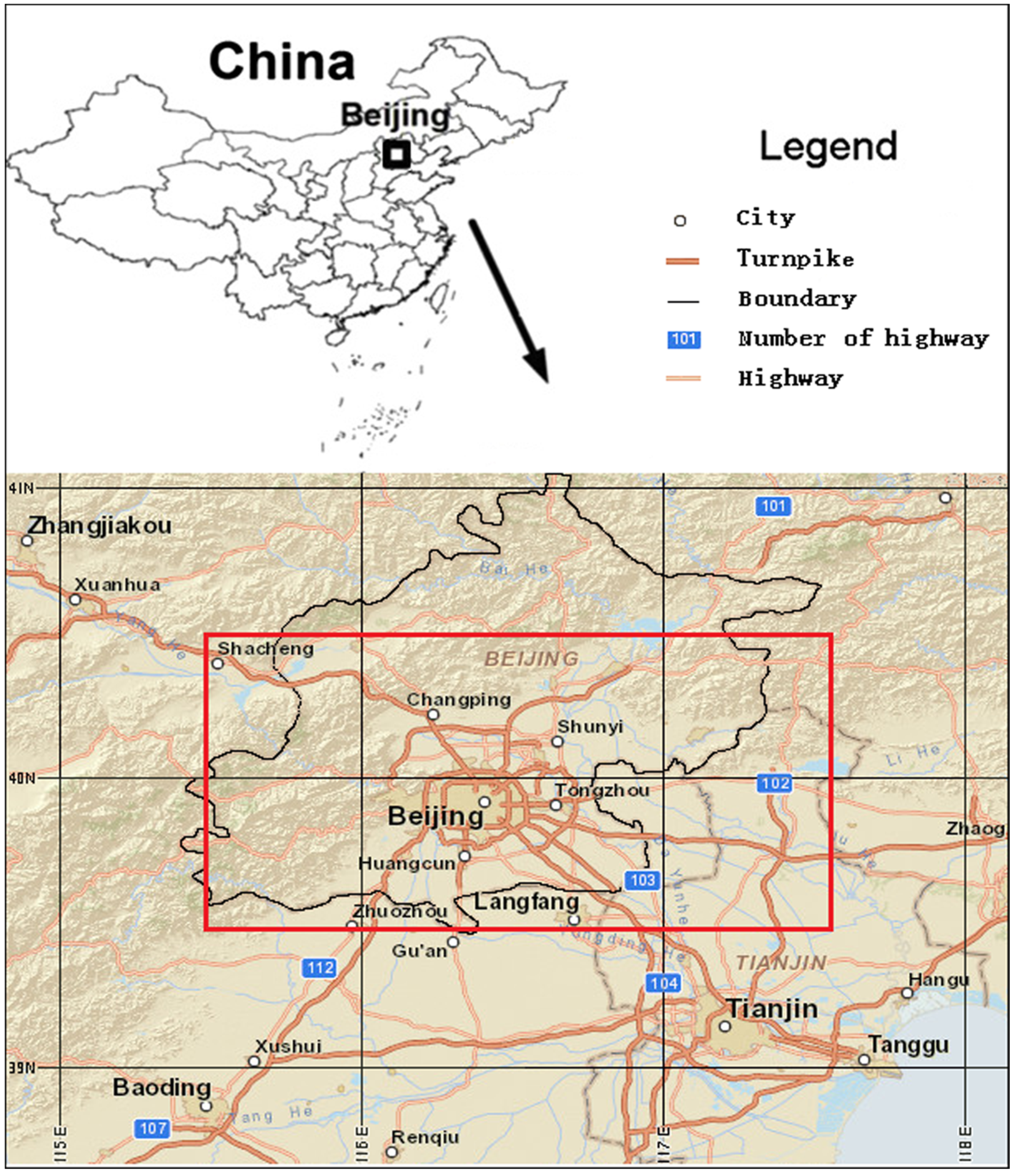
2.1. Study Area

To monitor PM2.5 concentrations using DMSP nighttime satellite images, we selected Beijing (Figure 1) as the study area for analysis. Beijing is situated in the eastern part of China, to the west of the Bohai Sea and covers more than 16,410 square kilometers.
Figure 1. The geographic location of the study area is indicated by the black square on the Chinese national map (upper). The study area (115.5°–117.5°E, 39.5°–40.5°N) is indicated by the red polygon (lower).
Atmosphere 06 00607 g001
Beijing is one of the largest metropolitan areas in the world. Rapid urban sprawl over the past 30 years has put tremendous pressure on the local and regional environment [34]. To improve air quality, the Chinese government implemented aggressive air pollution control measures in Beijing and surrounding areas. All on-road vehicles (including both trucks and passenger cars) that failed to meet the European Level IV emissions standards were banned from Beijing's roads. Mandatory restrictions were implemented to reduce the use of government vehicles and personal vehicles by ~20% by allowing these vehicles on the roads only on alternate days, based on license plate numbers. In addition to mobile sources, several heavily polluting industrial sources, such as power plants, were ordered to reduce their operating capacities or to completely shut down. Although great efforts have been made to control the air pollution, the PM levels remain much higher than the national air quality standard.

2.2. Data and General Procedures

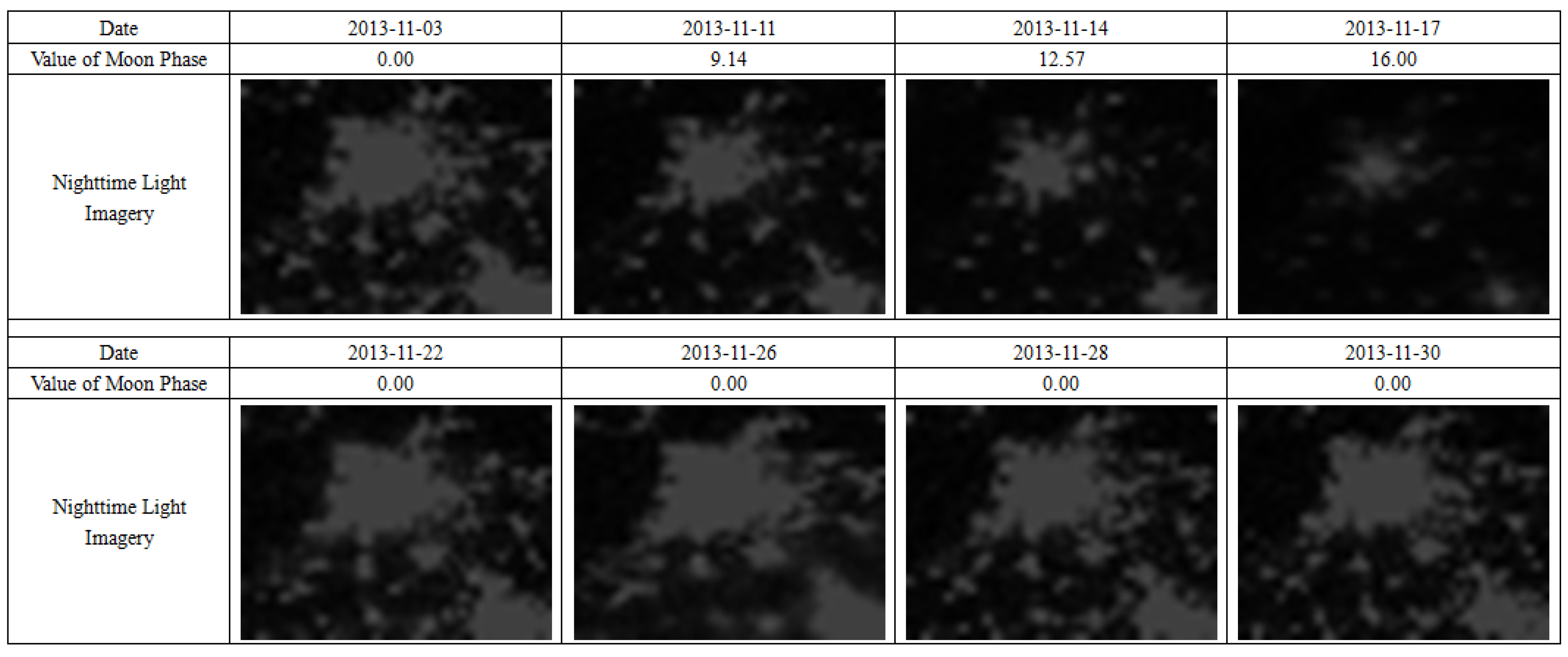
2.2.1. DMSP-OLS Nighttime Light Data

The DMSP-OLS operates satellites in sun-synchronous orbits with nighttime overpasses in the 8:00–10:00 p.m. range (local time) to map artificial lighting present on the Earth’s surface. The OLS is an oscillating scan system, with a swath width of 3000 km and 14 orbits per day; each OLS instrument can generate a complete coverage of nighttime data in a 24-h period. At night, the OLS has a photo-multiplier tube (PMT) to intensify visible-band light to observe faint sources of visible to near-infrared emissions [35].
In this study, we accessed the daily DMSP-OLS nighttime light (NTL) data products, which consist of 85 datasets from 9 October 2013 to 6 February 2014, without cloudy days and without days with snow on the ground. The data are organized into DMSP-OLS Nighttime Lights Global Composites (Version 4) and can be obtained from the National Geophysical Data Center (NGDC) website [36].

2.2.2. Daily PM2.5 Average Concentrations

We accessed the 120 datasets of daily air pollution index (API) for Beijing for the period between 9 October 2013 and 6 February 2014. These data were obtained from the Beijing Municipal Environmental Protection Bureau website [37].
When the primary pollutant was fine particles, the daily average PM2.5 concentrations were derived from the air pollution index (API) via the method presented in Table 1. The method is based on the Chinese Ambient Air Quality Standard (GB3095-2012) [11,38].

2.2.3. Phase of the Moon and Digitization

Step 1: We determined the phase of the moon between 9 October 2013 and 6 February 2014 based on the Internet Observatory of China website [39]. We then digitized the data using the following method: (1) a full moon day was assigned the value 16; (2) the waxing and waning of the moon were assigned the value 8; (3) the last day of a lunar month and the new moon day were assigned the value 0; and (4) the other days’ values were obtained via linear interpolation.
Table 1. Deriving the PM2.5 concentration from the API.
Range of AQI (x: no unit data)Range of PM2.5 Concentration (C:μg/m3)Formula
0 ≤ x ≤ 1000 ≤ C ≤ 75C = 75 × x/100
100 ≤ x ≤ 15075 ≤ C ≤ 115C = (x − 100) × (115 − 75)/(150 − 100) + 75
150 ≤ x ≤ 200115 ≤ C ≤ 150C = (x − 150) × (150 − 115)/(200 − 150) +115
200 ≤ x ≤ 300150 ≤ C ≤ 250C = (x − 200) × (250 − 150)/(300 − 200) + 150
300 ≤ x ≤ 400250 ≤ C ≤ 350C = (x − 300) × (350 − 250)/(400 − 300) + 250
400 ≤ x ≤ 500350 ≤ C ≤ 500C = (x − 400) × (500 − 350)/(500 − 400) + 350
500 = x500 ≤ CC = 500
Step 2: We also determined the time of the rising and setting of the moon between 9 October 2013 and 6 February 2014. These data were obtained from the CalSky website [40]. If the satellite’s passing time was not in the range between the rise and set of the moon, the days value was assigned the value 0.

2.2.4. LANDSAT-8 OLI-TIRS Data of Beijing

We accessed the 1 September 2013 LANDSAT-8 OLI-TIRS data for Beijing. The data set was provided by GSCloud, Computer Network Information Center, and Chinese Academy of Sciences [41].

2.2.5. Beijing Meteorological Data

We compiled the daily ground climate data for Beijing between 1 October 2013 and 1 February 2014 collected by the Chinese international exchange station. The data include temperature, relative humidity (RH), wind speed and barometric pressure, among other data sets. The data were provided by the National Meteorological Information Center of China [42].

2.3. Neural-Network Model Development

2.3.1. Data Pre-Processing Phase

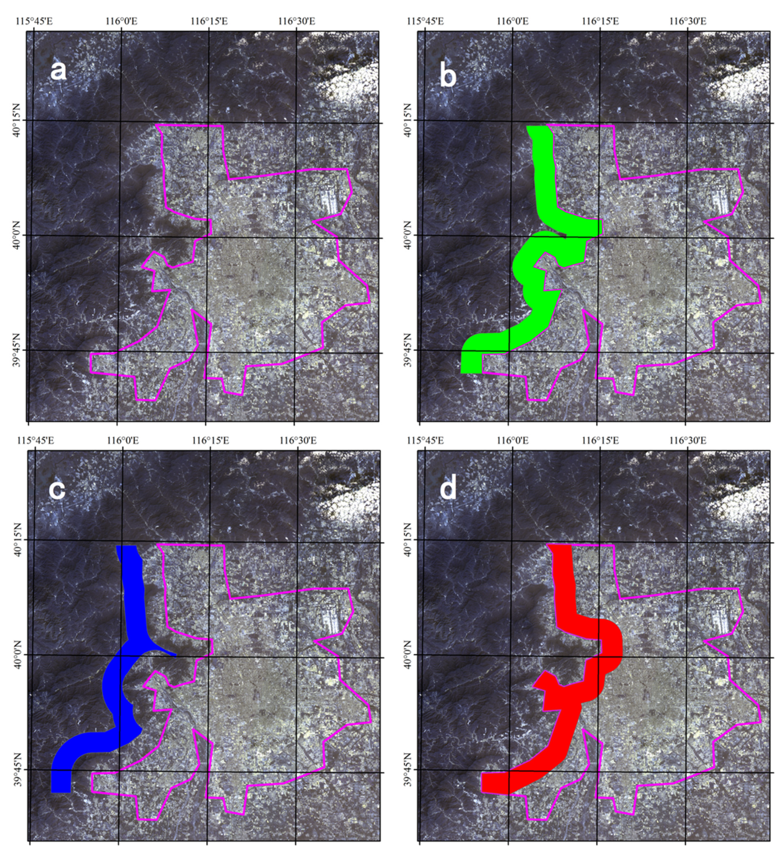
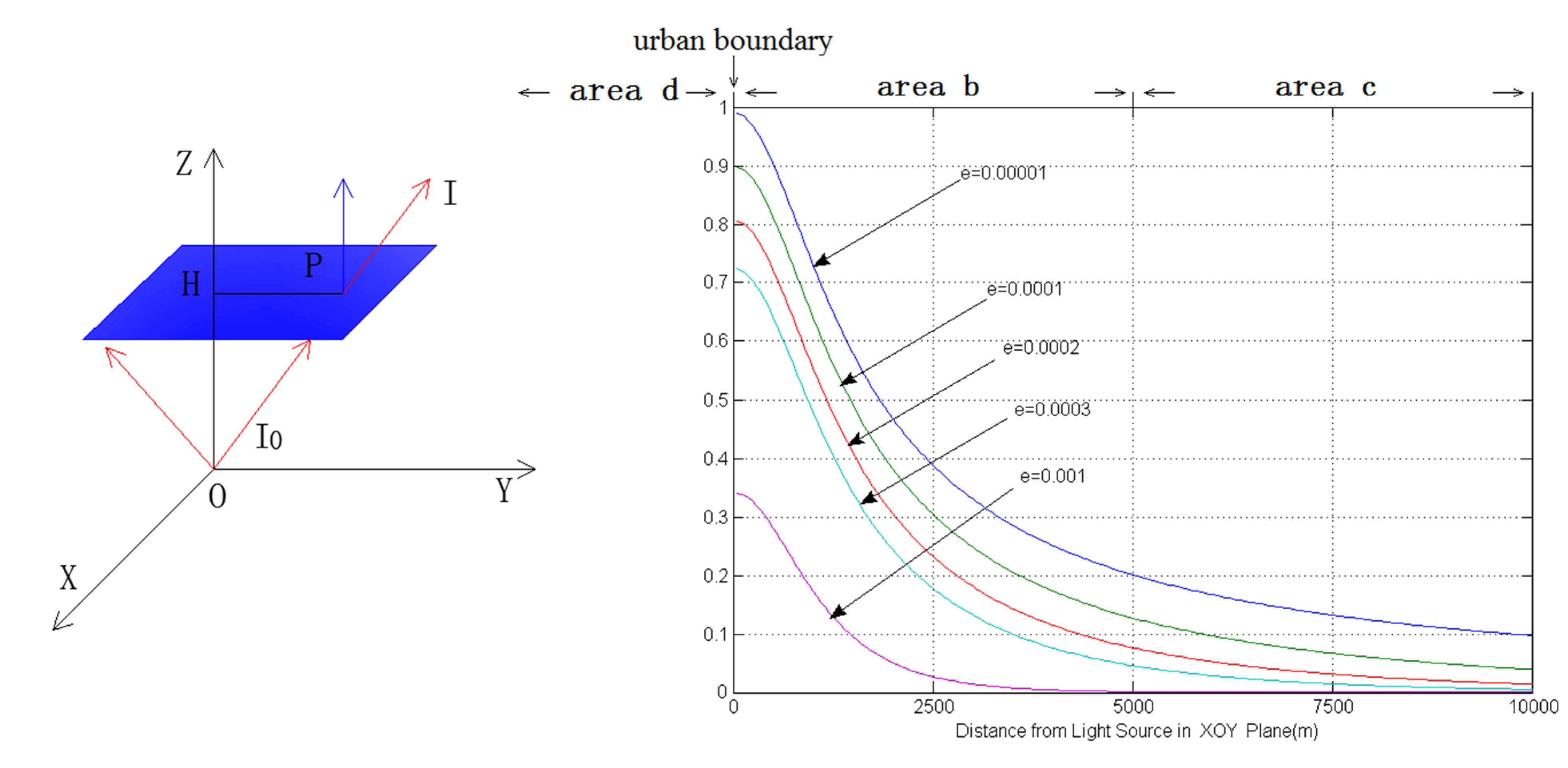
Division of the DMSP-OLS NTL Data into Four Regions

The phase of the moon has a significant influence on the gain settings of the OLS. The gain settings increase as the lunar illumination decreases. Higher gain settings are associated with larger numbers of detected pixels in the nighttime light imagery (Figure 2). During the darkest 10 nights of each lunar cycle, the effects of the along scan gain and bidirectional reflectance distribution function (BRDF) algorithms are minimized, and the gain reaches its maximum monthly level [43]. To avoid the influence of the moon, we selected the darkest nights of each lunar cycle. Thus, the night’s lunar phase was digitized with the value 0. Consequently, the 85 groups of available data decreased to 33 groups.
The primary objective of the on-orbit OLS gain control is the generation of consistent imagery of clouds at all scan angles for visual interpretation by Air Force meteorologists. In normal operations, the video digital gain amplifier (VDGA) is modified to track scene illumination predicted from lunar phase and elevation. The resulting base gains are modified every 0.4 ms by an onboard along-scan gain control (ASGC) algorithm [43]. The imagery presented herein was obtained under a computer control mode known as along-track gain control (ATGC), in which the VDGA gain remains at a fixed value throughout an entire scan [44]. Thus, each pixel in the same scanning line has the same magnification.
Figure 2. Relationship between the value of the moon phase and the nighttime light imagery. The top 4 days (3 November 2013, 11 November 2013, 14 November 2013 and 17 November 2013) demonstrate that the gain settings gradually increase as the lunar illumination decreases. Higher gain settings are associated with larger numbers of detected pixels in the nighttime light imagery. The lower 4 days (22 November 2013, 26 November 2013, 28 November 2013 and 30 November 2013) demonstrate that the gain settings reach maximum values during the darkest 10 nights of a lunar cycle.
Atmosphere 06 00607 g002
The spatial distribution of land use in Beijing includes mountainous areas, forest, and farmland to the west of downtown Beijing. We hypothesized that the urban area emits visible light at night, whereas the mountain, forest and farmland do not. Using visual interpretation, we circled the urban area of Beijing city (area a) using the LANDSAT-8 OLI-TIRS data. In addition to the urban core, three areas were defined according to the western boundary of urban area: one 5-km-wide strip extending westward from the western boundary, another 5-km-wide strip between 5 and 10 km from the western boundary, and a third 5-km-wide strip extending eastward from the western boundary (represented by areas b, c and d in Figure 3, respectively).
Using ArcGIS spatial analysis tools and the 4 defined regions, we divided the daily DMSP-OLS NTL data into four regions. We then summed the regional digital number (DN) values, which yielded SUM_ DNa, SUM_ DNb, SUM_ DNc, SUM_ DNd for areas a, b, c, and d, respectively.

PM2.5 Concentrations Data Corrected By Relative Humidity

Among the various meteorological factors, such as temperature, RH, wind speed and barometric pressure, RH has been determined to significantly affect air pollution levels [45].
In an air sample that is heated to 50 °C [46], the particles in the air sample are almost the “dry mass”. The PM2.5 concentrations measured by tapered-element oscillating microbalances (TEOM) are lower than in ambient air. Therefore, a proper RH correction should be introduced to reduce the impact of the variation in RH on the PM2.5 concentrations. Hence, we define the “RH_corrected PM2.5 concentration” as the “wet” PM2.5 concentration in the ambient air. This correction represents the “dry” PM2.5 concentration obtained under relatively dry conditions multiplied by a hygroscopic growth factor. Based on previous studies [16,47,48], the “RH_corrected PM2.5 concentration” can be written as follows:
R H _ c o r r e c t e d P M 2.5 c o n c e n t r a t i o n = d a i l y a v e r a g e P M 2.5 c o n c e n t r a t i o n 1 R H / 100  (1 < RH < 100)
Figure 3. The 4 daily NTL data regions. The purple polygon (a) is the urban boundary of Beijing. The green region (b) extends westward 5 km from the western boundary of the urban area. The blue region (c) extends westward 5 km from the western boundary of area b (i.e., between 5 and 10 km from the urban boundary). The red region (d) extends eastward 5 km from the western boundary of the urban area.
Atmosphere 06 00607 g003

2.3.2. Data Normalization

To avoid data saturation, the input variables in this study’s model were normalized based on their possible ranges using the following equation:
X n o r m = X i X min X max X min
where xi, xmin, xmax and xnorm are the input variable’s actual value, minimum value, maximum value and normalized value, respectively. The neural-network model’s output is also an indexed value that responds to the input variable. Using the following equation to de-normalize the indexed output value, we obtain a real-value output:
Y a i = Y min + Y n o r m ( Y max Y min )
where yai, ymin, ymax and ynorm are the output variable’s real value, minimum value, maximum value, and the indexed output value from the neural-network model, respectively.

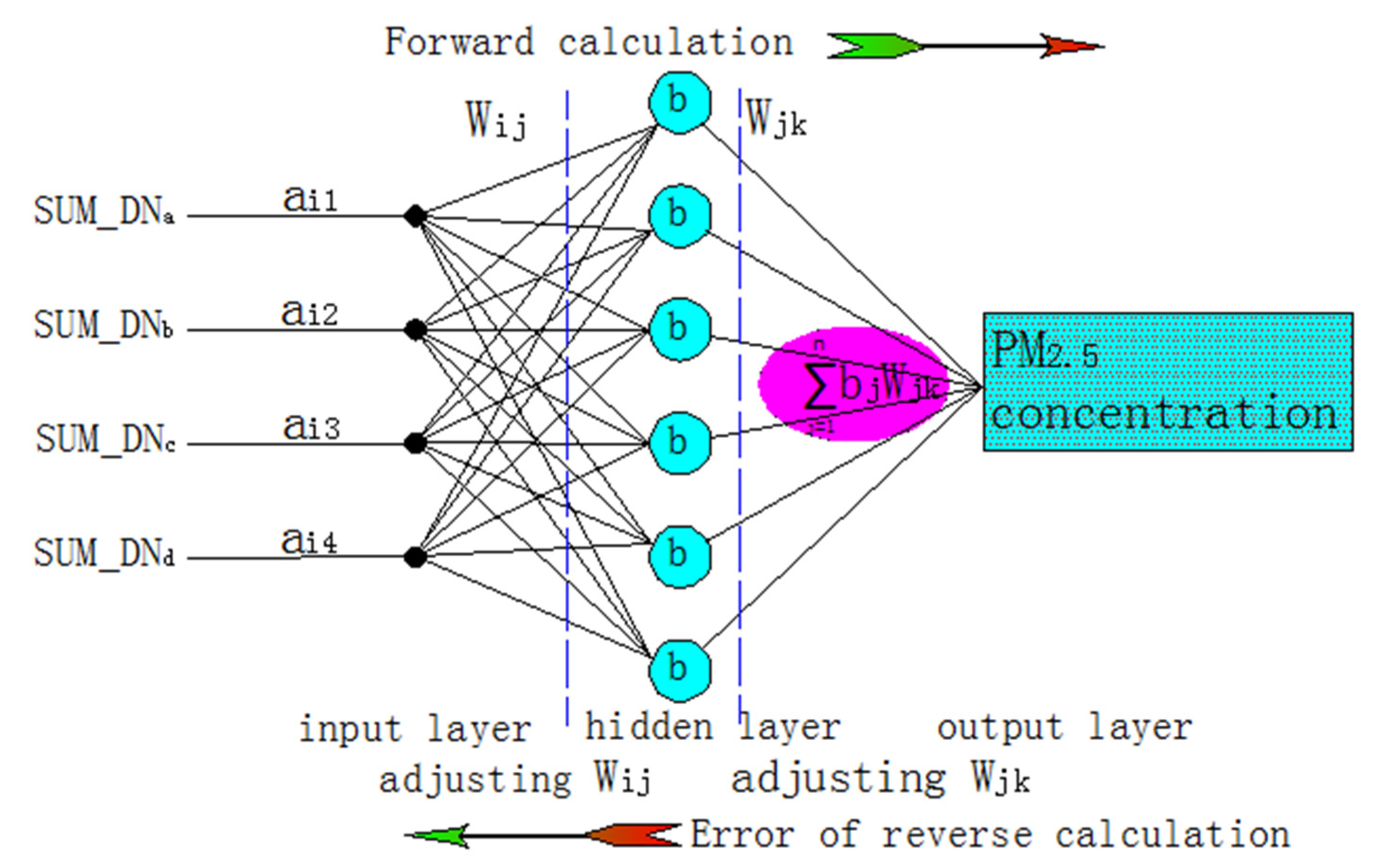
2.3.3. Model Building Phase

Artificial neural network (ANN) models have found wide applications, including prediction, classification, system modeling, signal processing, and noise filtering [49,50,51,52]. BP neutral networks are a popular neutral network architecture [49,50,51,52,53,54]. In this study, a BP neural-network model was established to estimate the RH_corrected PM2.5 concentrations. The input variables for the BP neural-network model were SUM_ DN.a, SUM_ DN b, SUM_ DN c and SUM_ DN d, and the output variable of this model was the RH_corrected PM2.5 concentration.
The topological structure of the BP neural-network model in this paper consisted of four input neurons in the input layer, one output neuron in the output layer and one hidden layer with six neurons. The flowchart of the 4-6-1 structure is shown in Figure 4.
Figure 4. The 4-6-1 topological structure of the BP neural-network model.
Atmosphere 06 00607 g004

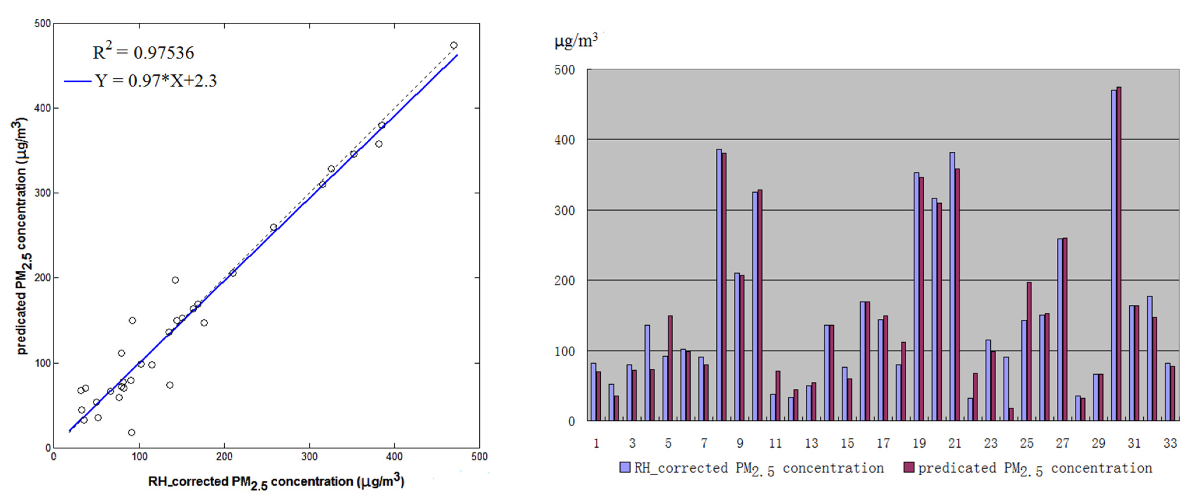
2.3.4. Model Evaluation Phase

Generally, root mean square error (RMSE) and average accuracy have been used to measure the performance of neural-network models [55]. In this study, the parameters were (i) RMSE; (ii) average accuracy (Pav); (iii) R2; (iv) mean bias error (MBE); and (v) index of agreement (IA). The five parameters were computed using Equations (4)–(8), respectively:
R M S E = i = 1 N ( y a i y m i ) 2 N 1
where yai and ymi are the output variable’s real value and the measured variable value, respectively, RMSE is the RMSE between the value of the output variable and measured variable, and N is the sample number. Lower RMSE values indicate better model performance.
P a v = i = 1 N P i N  and  P i = [ 1 | y a i y m i | y m i ]
where Pav and Pi are the average accuracy and the accuracy of the ith result. Pav provides information on the accuracy of the model using a given dataset. Values close to 1 indicate better model performance.
R 2 = [ i = 1 N ( y a i y a ¯ ) i = 1 N ( y m i y m ¯ ) ] 2 i = 1 N ( y a i y a ¯ ) 2 i = 1 N ( y m i y m ¯ ) 2
where R2, ym and ya are the correlation coefficient, average measured variable value and average actual output variable value, respectively. The R2 value represents the correlation between the predicted and measured variables. The predicted and measured variables are assumed to follow a normal distribution. R2 values range from 0 to 1. Higher correlation values represent stronger linear relationships between the actual and predicted variables.
M B E = i = 1 N ( y a i y m i ) N
where yai and ymi are the output variable’s real value and the measured variable value, respectively, and N is the sample number. Lower MBE values indicate better model performance.
I A = 1 i = 1 N ( y a i y m i ) 2 i = 1 N ( | y a i y m ¯ | + | y m i y m ¯ | ) 2
where yai, ymi and ym are the output variable’s real value, the measured variable value and average measured variable value, respectively, and N is the sample number. Values close to 1 indicate better model performance.

3. Results and Discussions

The architecture of the BP neural-network was 4-6-1, and the learning algorithm was a gradient descent BP algorithm, with the learning rate of 0.2 and a momentum coefficient of 0.2. The activation function was a sigmoid tangent function in the input layer and hidden layer and a sigmoid logistic function in the output layer. In total, 23 groups of data were used for training, five groups were used for verification purposes, and five groups were used for testing.
The R2 value of the correlation between the BP network model predictions and the RH_corrected PM2.5 concentrations was 0.975. The RMSE was 26.26 μg/m3 and the MBE value was −1.806 μg/m3, with a corresponding average PM2.5 concentration of 155.07 μg/m3. The Pav value was 0.796 and the IA value was 0.988. The predicted PM2.5 concentrations matched the RH_corrected PM2.5 concentrations well, as shown in Figure 5.
Figure 5. Correlation of the relative humidity corrected (RH_corrected) PM2.5 concentrations and the PM2.5 concentrations predicated by the BP neural-network.
Atmosphere 06 00607 g005
The BP network model using nighttime light data performs well in estimating the PM2.5 pollution degree of Beijing. The best results are obtained via the careful selection of regions in the DMSP-OLS nighttime light data.
Because the temporal difference between the 2013 Landsat 8 OLI-TIRS images and the 2013 nighttime light data is slight, we can compare these data sets to estimate the spatial consistency of urban areas. The lit areas of the city cover a larger area than the urban built-up areas (see Landsat 8 image). In addition, water bodies and urban forests are also illuminated in the DMSP-OLS data. This “blooming” phenomenon was also reported by other researchers [27,56]. The light intensity of the suburbs relative to the urban core contains information on the ground air’s extinction coefficient. Furthermore, the extinction coefficient can be used to estimate the particulate matter content in the air. Thus, the estimation of PM2.5 concentrations is feasible using DMSP-OLS data.
DMSP-OLS sensors capture images every day, but the daily imagery is affected by sensor noise, atmospheric and moonlight variations. The National Oceanic and Atmospheric Administration (NOAA) has attempted to minimize the sensor noise. By using DMSP-OLS data from nights with little or no moonlight, we have minimized the effects of the along-scan gain and bidirectional reflectance distribution function (BRDF) algorithms. Thus, the daily nighttime light data are comparable in terms of the effects of atmospheric variations.
The DMSP-OLS data provide an effective method for estimating extinction coefficient variations in ground air with PM pollution. PM pollution reduces the transmission capability of light, resulting in differences in spatial distribution of nighttime light data (Figure 6 [57]). We presumed that area d was a light-emitting region and that areas b and c were not. The upward luminous flux of areas b and c was radiated from area d. This process is complex and nonlinear. To solve this problem, the BP neural-network was selected to estimate the degree of PM2.5 pollution.
Figure 6. The sketch map (left) describes the position of a point light source and the surface to compute the luminous flux. Point O has a point light source with a light intensity of 1.0 unit (I0). The distance from point O to point H is 1076 meters (The aerosol scale height of Beijing in winter is 1076 meters [57]). A horizontal plane passes through point H and is perpendicular to the Z-axis; this plane is termed the Z = 1076 m Plane. Point P is on the Z = 1076 m Plane. The luminous flux through point P and parallel to the Z-axis is a function of two parameters. One is the distance from point P to point H; the other is the extinction coefficient of atmosphere. The line chart (right) describes the function for a different situation. The X-axis is the distance from point P to point H, and the Y-axis is the upward luminous flux through point P and parallel to the Z-axis. The label e is the extinction coefficient of atmosphere. Area d was a light-emitting region, and areas b and c were not. The upward luminous flux of areas b and c was radiated from area d.
Atmosphere 06 00607 g006
The primary data set of this research is DMSP imagery that provides information on the ground air’s extinction coefficient. We proposed an effective method to split DMSP imagery, intentionally highlighting the differences in the spatial distribution of NTL data. Future studies should focus on the quantitative relationship between PM pollution and DMSP-OLS data throughout the lunar cycle. New sources of high spatial resolution nighttime images, such as the NPP-VIIRS Nighttime Light Data [58,59,60], the EROS-B commercial satellite data [61] and aerial photography [62], may allow for better estimation methods and results.
Meteorological conditions are a significant driver of local ambient air pollution concentrations, especially wind speed and relative humidity. Wind can disperse particulate matter but cannot influence the extinction coefficient. Therefore, relative humidity was used to correct the daily “dry” PM2.5 concentrations. DMSP-OLS data can be obtained only in clear and cloudless days. Other days were not included in this study. Nighttime inversion conditions and upper air meteorological conditions (turbulence, etc.) may impact the light transmission from the ground to satellite, and we will consider these factors in the future studies.

4. Conclusions

By selecting Beijing, the largest and fastest developing city in the world, as the study area, this research synthesizes RS and GIS techniques and estimates the PM2.5 pollution degree of the ground-level atmosphere. This study proposed a simple monitoring method of nighttime PM2.5 concentrations.
The innovation of this research lies in the selection of spatial regions in the data set. Based on the land use type to the west of Beijing, the distribution characteristics of the land and the light scattering from urban to suburban, four regions were defined from which to extract the nighttime light data, instead of constructing various indices from the entire DMSP-OLS imagery data set. The relative numerical ratio of the data extracted from these four regions reflects the extinction coefficient of the atmosphere, and this extinction coefficient can be used to retrieve the aerosol concentration.
Our method and results can provide guidance for developing and implementing environmental conservation planning. Furthermore, these data can assist government agencies in determining PM pollution control areas, initiating regulation projects, and undertaking nighttime environmental purifying measures.

Acknowledgments

We would like to thank NOAA-NGDC for providing the DMSP data and the Beijing Environmental Protection Bureau for the PM2.5 pollution data used in this research. The authors are grateful to the anonymous reviewers for their insightful and helpful comments, which have improved the manuscript.

Author Contributions

Runya Li and Xiangnan Liu conceived and supervised the research topic. Runya Li and Xuqing Li proposed the methods and processed the data. Runya Li analyzed the results and wrote the paper. All authors read and approved the submitted manuscript, agreed to be listed and accepted the version for publication.

Conflicts of Interest

The authors declare no conflict of interest.

References

  1. Kaufman, Y.J.; Tanré, D.; Boucher, O. A satellite view of aerosols in the climate system. Nature 2002, 419, 215–223. [Google Scholar] [CrossRef] [PubMed]
  2. WHO (World Health Organization). Air Quality Guidelines for Europe, 2nd ed.; Chapter 7, WHO Regional Publications, European Series: Geneva, Switzerland, 2000; Volume 91. [Google Scholar]
  3. Pope, C.A. Review: Epidemiological basis for particulate air pollution health standards. Aerosol Sci. Technol. 2000, 32, 4–14. [Google Scholar] [CrossRef]
  4. Wallace, L. Correlations of personal exposure to particles with outdoor air measurement: A review of recent studies. Aerosol Sci. Technol. 2000, 32, 15–25. [Google Scholar] [CrossRef]
  5. Kan, H.D.; Chen, B.H. Analysis of exposure-response relationships of air particulate matter and adverse health outcomes in China. J. Environ. Health 2002, 19, 422–424. (In Chinese) [Google Scholar]
  6. Li, J.J.; Shao, L.Y.; Yang, S.S. Adverse effect mechanisms of inhalable particulate matters. J. Environ. Health 2006, 3, 185–188. (In Chinese) [Google Scholar]
  7. Samoli, E.; Peng, R.; Ramsay, T.; Pipikou, M.; Touloumi, G.; Dominici, F.; Burnett, R.; Cohen, A.; Krewski, D.; Samet, J.; et al. Acute effects of ambient particulate matter on mortality in Europe and North America: Results from the APHENA study. Environ. Health. Perspect. 2008, 116, 1480–1486. [Google Scholar] [CrossRef] [PubMed]
  8. Nastos, P.T.; Paliatsos, A.G.; Anthracopoulos, M.B.; Roma, E.S.; Priftis, K.N. Outdoor particulate matter and childhood asthma admissions in Athens, Greece: A time-series study. Environ. Health 2010, 9. [Google Scholar] [CrossRef]
  9. Li, C.C.; Mao, J.T.; Lau, A.K.; Liu, X.Y.; Liu, G.Q.; Zhu, A. Research on the air pollution in Beijing and its surroundings with MODIS AOD product. Chin. J. Atmos. Sci. 2003, 27, 869–880. (In Chinese) [Google Scholar]
  10. Song, Y.; Tang, X.Y.; Fang, C.; Zhang, Y.; Hu, M.; Zeng, L.; Li, C.; Mao, J.; Michael, B. Relationship between the visibility degradation and particle pollution in Beijing. Acta Sci. Circumst. 2003, 23, 468–471. (In Chinese) [Google Scholar]
  11. The Ministry of Environmental Protection of the People’s Republic of China. Chinese National Standards: Ambient Air Quality Standards (GB3095–2012). Available online: http://bz.mep.gov.cn/bzwb/dqhjbh/dqhjzlbz/201203/t20120302_224165.htm (accessed on 1 May 2014). (In Chinese)
  12. Remer, L.A.; Kaufman, Y.J.; Tanré, D.; Mattoo, S.; Chu, D.A.; Martins, J.V.; Li, R.-R.; Ichoku, C.; Levy, R.C.; Kleidman, R.G.; et al. The MODIS aerosol algorithm, products, and validation. J. Atmos. Sci. 2005, 62, 947–973. [Google Scholar] [CrossRef]
  13. King, M.D.; Kaufman, Y.J.; Tanré, D. Remote sensing of tropospheric aerosols from space: Past, present, and future. B Am. Meteorol. Soc. 1999, 80, 2259. [Google Scholar] [CrossRef]
  14. Chu, D.A.; Kaufman, Y.J.; Zibordi, G.; Chern, J.D.; Mao, J.; Li, C.C.; Holben, B.N. Global monitoring of air pollution over land from the Earth Observing System—Terra Moderate Resolution Imaging Spectroradiometer (MODIS). J. Geophys. Res. 2003, 108, ACH4-1–ACH4-18. [Google Scholar]
  15. Wang, J.; Christopher, A. Intercomparison between satellite-derived aerosol optical thickness and PM2.5 mass: Implications for air quality studies. Geophys. Res. Lett. 2003, 30, 1–4. [Google Scholar]
  16. Li, C.C.; Mao, J.T.; Lau, A.K.; Yuan, Z.B.; Wang, M.H.; Liu, X.Y. Application of MODIS satellite product to the air pollution research in Beijing. Sci. China Ser. D 2005, 35, 177–186. [Google Scholar]
  17. Liu, Y.; Sarnat, J.A.; Kilaru, V.; Jacob, D.J.; Koutrakis, P. Estimating ground-level PM2.5 in the eastern United States using satellite remote sensing. Environ. Sci. Technol. 2005, 39, 3269–3278. [Google Scholar] [CrossRef] [PubMed]
  18. Doll, C.N.H.; Muller, J.P.; Morley, J.G. Mapping regional economic activity from night-time light satellite imagery. Ecol. Econ. 2006, 57, 75–92. [Google Scholar] [CrossRef]
  19. Elvidge, C.D.; Sutton, P.C.; Ghosh, T.; Tuttle, B.T.; Baugh, K.E.; Bhaduri, B.; Bright, E. A global poverty map derived from satellite data. Comp. Geosci. 2009, 35, 1652–1660. [Google Scholar] [CrossRef]
  20. Li, X.; Xu, H.; Chen, X.; Li, C. Potential of NPP-VIIRS nighttime light imagery for modeling the regional economy of China. Remote Sens. 2013, 5, 3057–3081. [Google Scholar] [CrossRef]
  21. Chen, X.; Nordhaus, W.D. Using luminosity data as a proxy for economic statistics. Proc. Natl. Acad. Sci. USA 2011, 108, 8589–8594. [Google Scholar] [CrossRef] [PubMed]
  22. Henderson, V.; Storeygard, A.; Weil, D.N. A bright idea for measuring economic growth. Am. Econ. Rev. 2011, 101, 194–199. [Google Scholar] [CrossRef] [PubMed]
  23. Ghosh, T.; Anderson, S.; Powell, R.L.; Sutton, P.C.; Elvidge, C.D. Estimation of Mexico’s informal economy and remittances using nighttime imagery. Remote Sens. 2009, 1, 418–444. [Google Scholar] [CrossRef]
  24. Zhuo, L.; Ichinose, T.; Zheng, J.; Chen, J.; Shi, P.J.; Li, X. Modelling the population density of China at the pixel level based on DMSP/OLS non-radiance-calibrated night-time light images. Int. J. Remote Sens. 2009, 30, 1003–1018. [Google Scholar] [CrossRef]
  25. Bharti, N.; Tatem, A.J.; Ferrari, M.J.; Grais, R.F.; Djibo, A.; Grenfell, B.T. Explaining seasonal fluctuations of measles in Niger using nighttime lights imagery. Science 2011, 334, 1424–1427. [Google Scholar] [CrossRef] [PubMed]
  26. Zhang, Q.L.; Seto, K.C. Mapping urbanization dynamics at regional and global scales using multi-temporal DMSP/OLS nighttime light data. Remote Sens. Environ. 2011, 115, 2320–2329. [Google Scholar] [CrossRef]
  27. Small, C.; Pozzi, F.; Elvidge, C.D. Spatial analysis of global urban extent from DMSP-OLS night lights. Remote Sens. Environ. 2005, 96, 277–291. [Google Scholar] [CrossRef]
  28. Zhang, Q.; Seto, K. Can night-time light data identify typologies of urbanization? A global assessment of successes and failures. Remote Sens. 2013, 5, 3476–3494. [Google Scholar] [CrossRef]
  29. Prasad, V.K.; Kant, Y.; Gupta, P.K.; Elvidge, C.; Badarinath, K. Biomass burning and related trace gas emissions from tropical dry deciduous forests of India: A study using DMSP-OLS data and ground-based measurements. Int. J. Remote Sens. 2002, 23, 2837–2851. [Google Scholar] [CrossRef]
  30. Waluda, C.; Yamashirob, C.; Elvidge, C.; Hobson, V.; Rodhouse, P. Quantifying light-fishing for Dosidicus gigas in the eastern Pacific using satellite remote sensing. Remote Sens. Environ. 2004, 91, 129–133. [Google Scholar] [CrossRef]
  31. Chand, T.R.K.; Badarinath, K.V.S.; Elvidge, C.D.; Tuttle, B.T. Spatial characterization of electrical power consumption patterns over India using temporal DMSP-OLS night-time satellite data. Int. J. Remote Sens. 2009, 30, 647–661. [Google Scholar] [CrossRef]
  32. Agnew, J.; Gillespie, T.W.; Gonzalez, J.; Min, B. Baghdad nights: Evaluating the US military “surge” using nighttime light signatures. Environ. Plan. A 2008, 40, 2285–2295. [Google Scholar] [CrossRef]
  33. Aubrecht, C.; Elvidge, C.; Longcore, T.; Rich, C.; Safran, J.; Strong, A.; Eakin, C.; Baugh, K.; Tuttle, B.; Howard, A. A global inventory of coral reef stressors based on satellite observed nighttime lights. Geocarto Int. 2008, 23, 467–479. [Google Scholar] [CrossRef]
  34. Liu, Y.; He, K.B.; Li, S.S.; Wang, Z.X.; David, C.C.; Petros, K. A statistical model to evaluate the effectiveness of PM2.5 emissions control during the Beijing 2008 Olympic Games. Environ. Int. 2012, 44, 100–105. [Google Scholar] [CrossRef] [PubMed]
  35. Elvidge, C.D.; Baugh, K.E.; Kihn, E.A.; Kroehl, H.W.; Davis, E.R. Mapping city lights with nighttime data from the DMSP operational linescan system. Photogramm. Eng. Remote Sens. 1997, 63, 727–734. [Google Scholar]
  36. NGDC. The National Geophysical Data Center. Available online: http://maps.ngdc. noaa.gov/viewers/dmsp_mosaic/ (accessed on 6 February 2014).
  37. The Beijing Municipal Environmental Protection Bureau. Available online: http://wsbs.bjepb.gov.cn/air2008/Air.aspx (accessed on 8 February 2014).
  38. The Ministry of Environmental Protection of the People’s Republic of China. Chinese National Environmental Protection Standards: Technical Regulation on Ambient Air Quality Index (on trial) (HJ 633–2012). Available online: http://bz.mep.gov.cn/bzwb/dqhjbh/jcgfffbz/201203/t20120302_224166.htm (accessed on 1 May 2014). (In Chinese)
  39. The Internet Observatory of China. Available online: http://www.astron.ac.cn/list-72-1.htm (accessed on 10 February 2014).
  40. The CalSky website. Available online: http://www.calsky.com/cs.cgi (accessed on 10 February 2014).
  41. GSCloud, Computer Network Information Center, Chinese Academy of Sciences. Available online: http://www.gscloud.cn/ (accessed on 1 May 2014).
  42. The National Meteorological Information Center of China. Available online: http://cdc.nmic.cn/ (accessed on 1 March 2015).
  43. Elvidge, C.D.; Baugh, K.E.; Dietz, J.B.; Bland, T.; Sutton, P.C.; Herbert, W.K. Radiance Calibration of DMSP-OLS Low-Light Imaging Data of Human Settlements. Remote Sens. Environ. 1999, 68, 77–88. [Google Scholar] [CrossRef]
  44. Thomas, A. Croft. The Brightness of Lights on Earth at Night, Digitally Recorded by DMSP Satellite. Available online: http://ngdc.noaa.gov/eog/dmsp_docs.html (accessed on 1 May 2014).
  45. Kit, Y.C.; Le, J. Identification of significant factors for air pollution levels using a neural network based knowledge discovery system. Neurocomputing 2003, 99, 564–569. [Google Scholar]
  46. Lu, F.; Liu, J.G.; Lu, Y.H.; Zhan, K.; Wang, Y.P.; Chen, J. Design of real-time ambient particulate monitoring system based on TEOM technology. J. Atmos. Environ. Opt. 2007, 2, 361–365. [Google Scholar]
  47. Kotchenruther, R.A.; Hobbs, P.V.; Hegg, D.A. Humidification factors for atmospheric aerosols off the mid-Atlantic coast of the United States. J. Geophys. Res. 1999, 104, 2239–2251. [Google Scholar] [CrossRef]
  48. Im, J.; Saxena, V.K.; Wenny, B.N. An assessment of hygroscopic growth factors for aerosols in the surface boundary layer for computing direct radiative forcing. J. Geophys. Res. 2001, 106, 20213–20224. [Google Scholar] [CrossRef]
  49. Pachepsky, V.; Timlin, A.D.; Varallyay, G. Artificial neural networks to estimates oil water retention from easily measurable data. Soil Sci. Soc. Am. J. 1996, 60, 727–733. [Google Scholar] [CrossRef]
  50. Pal, N.R.; Pal, S.; Das, J.; Majumdar, K. SOFM-MLP: A hybrid neural network for atmospheric temperature prediction. IEEE Trans. Geosci. Remote. Sens. 2003, 41, 2783–2791. [Google Scholar] [CrossRef]
  51. Plate, T.; Bert, J.; Grace, J.; Band, P. Visualizing the function computed by a feed forward neural network. Neural Comput. 2000, 12, 1355–1370. [Google Scholar] [CrossRef] [PubMed]
  52. Tumbo, S.D.; Wagner, D.G.; Heinemann, P.H. Hyperspectral-based neural network for predicting chlorophyll status in corn. T. ASAE 2002, 45, 825–832. [Google Scholar]
  53. Ali, M.M.; Swain, D.; Weller, R.A. Estimation of ocean subsurface thermal structure from surface parameters: A neural network approach. Geophys. Res. Lett. 2004, 31, L20308. [Google Scholar] [CrossRef]
  54. Moustris, K.P.; Larissi, I.K.; Nastos, P.T.; Koukouletsos, K.V.; Paliatsos, A.G. Development and Application of Artificial Neural Network Modeling in Forecasting PM10 Levels in a Mediterranean City. Water Air Soil Pollut. 2013, 224, 1–11. [Google Scholar] [CrossRef]
  55. Gautam, R.; Panigrahi, S.; Franzen, D. Neural network optimization of remotely sensed maize leaf nitrogen with a genetic algorithm and linear programming using five performance parameters. Biosyst. Eng. 2006, 95, 359–370. [Google Scholar] [CrossRef]
  56. Henderson, M.; Yeh, E.T.; Gong, P.; Elvidge, C.; Baugh, K. Validation of urban boundaries derived from global night-time satellite imagery. Int. J. Remote Sens. 2003, 24, 595–609. [Google Scholar] [CrossRef]
  57. He, X.; Deng, Z.Z.; Li, C.C.; Alexis, K.L.; Wang, M.H.; Liu, X.Y.; Mao, J.T. Research on Application of MODIS aerosol optical thickness products in the ground PM10 monitoring. Acta Sci. Nat. Univ. Pekin. 2010, 2, 178–184. (In Chinese) [Google Scholar]
  58. Elvidge, C.D.; Baugh, K.E.; Zhizhi, M.; Hsu, F.-C. Why VIIRS data are superior to DMSP for mapping nighttime lights. Proc. Asia Pac. Adv. Netw. 2013, 35, 62–69. [Google Scholar] [CrossRef]
  59. Miller, S.D.; Straka, W.; Mills, S.P.; Elvidge, C.D.; Lee, T.F.; Solbrig, J.; Walther, A.; Heidinger, A.K.; Weiss, S.C. Illuminating the capabilities of the suomi national polar-orbiting partnership (NPP) visible infrared imaging radiometer suite (VIIRS) day/night band. Remote Sens. 2013, 5, 6717–6766. [Google Scholar] [CrossRef]
  60. Kaifang, S.; Bailang, Y.; Yixiu, H.; Yingjie, H.; Bing, Y.; Zuoqi, C.; Liujia, C.; Jianping, W. Evaluating the Ability of NPP-VIIRS Nighttime Light Data to Estimate the Gross Domestic Product and the Electric Power Consumption of China at Multiple Scales: A Comparison with DMSP-OLS Data. Remote Sens. 2014, 6, 1705–1724. [Google Scholar] [CrossRef]
  61. Noam, L.; Kasper, J.; Jorg, M.H.; Stuart, P. A newsource for high spatial resolution night time images—The EROS-B commercial satellite. Remote Sens. Environ. 2014, 149, 1–12. [Google Scholar] [CrossRef]
  62. Christopher, C.M.K.; Stefanie, G.; Helga, K.; Alejandro, S.M.; Jaime, Z.; Jürgen, F.; Franz, H. High-Resolution Imagery of Earth at Night: New Sources, Opportunities and Challenges. Remote Sens. 2015, 7, 1–23. [Google Scholar]

