Evaluating the Effects of Urbanization Evolution on Air Temperature Trends Using Nightlight Satellite Data


1
Department of Environment, Land and Infrastructure Engineering, Politecnico di Torino, 10129 Torino, Italy
2
Department of Civil, Chemical, Environmental and Materials Engineering, Università di Bologna, 40136 Bologna, Italy
*
Author to whom correspondence should be addressed.
Atmosphere 2019, 10(3), 117; https://doi.org/10.3390/atmos10030117
Submission received: 21 December 2018
/
Revised: 26 February 2019
/
Accepted: 26 February 2019
/
Published: 4 March 2019
(This article belongs to the Section Biometeorology)
Abstract
:Confounding factors like urbanization and land-use change could introduce uncertainty to the estimation of global temperature trends related to climate change. In this work, we introduce a new way to investigate the nexus between temporal trends of temperature and urbanization data at the global scale in the period from 1992 to 2013. We analyze air temperature data recorded from more than 5000 weather stations worldwide and nightlight satellite measurements as a proxy for urbanization. By means of a range of statistical methods, our results quantify and outline that the temporal evolution of urbanization affects temperature trends at multiple spatial scales with significant differences at regional and continental scales. A statistically significant agreement in temperature and nightlight trends is detected, especially in low and middle-income regions, where urbanization is rapidly growing. Conversely, in continents such as Europe and North America, increases in temperature trends are typically detected along with non-significant nightlight trends.
1. Introduction
The urban transition leads to alterations in landscape conditions and to important modifications in the urban climate, along with several environmental problems e.g., on water use and quality, on the generation of air pollution, and on the production of solid waste and sewage [1,2]. Because of rapid urbanization growth, even more considerable impacts are expected on a broader scale and especially in developing countries, like higher consumption of energy, goods, services, and resources demand, which have the potential for greater negative impacts on global environments and ecosystems [3,4,5,6,7]. Changes in food supplies, freshwater resources, and increase in extreme weather events (e.g., heatwaves and droughts) are expected to lead to several consequences on human health in terms of e.g., heat stress, cardio-respiratory, and infectious diseases [2,8]. In this regard, we must also consider that 55% of the world population is residing in urban areas in 2018, which is projected to reach 68% by 2050 [9]. In the context of global climate change, it is crucial to better investigate how urban growth affects temperature record trends to consistently attribute the causes of observed warming at wider scales [10,11,12,13,14,15,16].
The impact of urbanization on near surface temperatures has been investigated since the 1980s [17,18]. These studies suggested that a proportion of global warming observed on the last century timescale could be related to local warming induced by urbanization. Rapid urban growth has resulted in the expansion of built-up areas in and around cities, particularly for nations and regions experiencing demographic expansion. This plays a crucial role in the near-surface warming and on temperature measurements [13,19,20,21]. This process is known to affect the planetary boundary layer, to drive local climate changes, and to lead to the relative increase in temperature within the urban area [13,19,20] contributing to the so-called Urban Heat Island (UHI) effect within cities. The UHI effect identifies a sort of microclimate within cities, which leads to a difference of temperature between urban and surrounding non-urban areas, characterized by higher and lower temperatures, respectively, particularly during the night time [13,22]. UHI effects could be mainly ascribed to solar heat retention by building materials (having low albedo and high heat capacity), obstruction of longwave emission by the built environment, changes in land cover and urban geometries (e.g., reduced vegetation in urban areas) causing a generalized reduced evapotranspiration, and anthropogenic heat emissions (e.g., air conditioning, cars, and industrial facilities) [23,24,25]. Additionally, weather and local topographical characteristics contribute to the UHI effect as well [13,26]. As an example, studies suggest that land-sea interactions induce horizontal thermal advection while mountain landscapes are dominated by vertical advection [16,27].
The UHI measurement can be defined for different layers of the urban atmosphere and even surfaces. Since their underlying mechanisms and related measurements are different, it is, thus, important to distinguish between different urban heat islands [18]. Surface UHI refers to the land surface temperature specifically [5] while the atmospheric UHI considers the land air temperature as measured by land-based weather stations [15]. Because land air temperature is commonly used in climate warming analyses, in this paper, we consider atmospheric UHI only.
Previous works highlight how UHI affects the planetary boundary layer and how urban-atmospheric interactions control urban-induced impacts not only at the local scale (i.e., individual cities), but also over regional scales [26,28]. For instance, Georgescu et al. [28] calculated that urban expansion, separate from greenhouse gas-induced climate change, is projected to increase the near-surface temperature up to 2 °C at both a local and regional scale. More recent work has advanced this calculation by looking at the dynamic interaction and relative impact of urban to climate change effects on the near surface temperature through the 24-hour day/night period [29]. Urban extents and shaping impose different dynamics on urbanization-induced warming depending on spatial regional and geographic patterns [27,30]. Based on recent findings [20], the urban area size alone explains nearly 87% of UHI variance, with significant spatial and temporal variation over large areas. At the local level, the contribution of UHI to global warming during the summer is locally important, therefore originating immediate critical situations for human health and well-being [31,32]. At the regional level, urban warming is found to exhibit more relevant effects after some years of urban expansion [27]. Land cover spatial patterns are known to control UHI variation with higher values across regions with homogeneous land cover [20]. Recent regional-scale findings in the US show a marked heterogeneity in subnational temperature trends between large cities in Northeastern and Southern regions of the country. Higher UHI rates are typical of colder or high latitude regions, characterized by large urban areas surrounded by forested biomes. In contrast, southern urban ecosystems and urban areas built in desert-like environments are characterized by lower UHI rates [20,33,34]. The effects of urban expansion on the local climate were also investigated in Asia [35]. For instance, in China, notable regional effects are found during the earlier stage of the urban polycentric sprawl, whereas more drying effects and built-environment warming are locally reinforced in concentrated urbanized areas [27]. In Europe, a recent study on the largest 5000 urban agglomerations reveals that the urban size is the main determinant of UHI and local warming, which is followed by city compactness (i.e., single-centric or poly-centric cities) [36].
How urbanization could influence the assessment of global warming trends has not been thoroughly inspected so far [13,37]. Since the urban population is expected to increase in the future [2], the effect of urbanization trends on local and global warming is a key issue from the climate change perspective. In this regard, it is crucial to quantitatively assess the amplification of global temperature trends by urbanization i.e., to estimate to what extent large urbanized areas may be amplifying warming attributed to climate change on a global scale [34].
Recently, several studies were conducted in order to account and compensate for the effect of urban warming when estimating large scale temperature trends [11,14,15]. Global warming trend analyses are conducted, for example, using adjusted urban temperature data, by comparing observations to the sea surface temperature [11], comparing temperature values in different weather conditions [38], or removing sites with suspected urban warming from global [11] and regional warming analyses [39]. However, very often, the poor spatial coverage of the weather stations network does not guarantee the possibility to compare urban stations with the corresponding rural ones [40]. Most weather station networks are located in heavily anthropized sites [13,15]. Rapid urbanization makes the classification between urban and rural areas difficult in some cases [34].
New techniques and approaches could be helpful in detecting relationships and feedbacks between air temperature and land-use changes. These efforts result in independent and relatively accurate estimates of urban shape and extent. Remote-sensing products, which are primarily MODIS-500 maps [41,42,43,44], Landsat data [45], satellite night time images [3,46], and Synthetic Aperture Radar (SAR) data [47], are widely used to map global urban extent and to identify and geo-localize rural and urban stations [15,39]. In recent studies [46], day–night composites combine nightlights and Landsat to show consistencies in land cover and nightlights brightness. Other relevant works spatially assess the UHI signature on land surface temperature amplitude and its mutual relations with development size, intensity, and in different biomes, for over 3000 cities worldwide combining MODIS and night-time lights products i.e., a nightlight based impervious surface area (ISA) [48]. Nightlight ISA and Landsat ISA for cities in the continental US are first compared to bridge from previous studies. Results highlight significant positive relationships between UHI magnitude, ecological setting and ISA, and that nightlights are good estimators of urban sprawl and are more objective than methods based on population density. Zhou et al. [3] develop a method to map urban extent from nightlights on a global scale and compare it at the pixel level and regionally with five other widely used global urban products, including MODIS [43], GlobCover [49], and GLC2000 [50]. Results show that the nightlight map produced by the author is in high agreement with the other global urban area map products. Bagan and Yamagata [51] also show that the combined use of land cover data and nightlights are both good predictors of population density in Japan. On a local scale, recent studies [52] assess the properties of the temperature station network and the potential urban influence on temperature records by means of land cover, population density, and nightlights at an increasing buffer around the weather station. The three methods are found to be highly correlated, which indicates that nightlights and population density are good proxies of urban areas.
Thus, based on comparison with other existing global urban maps, night-time satellite images are demonstrated to be a good proxy of urban extent and allows for temporal dynamics analyses of urban areas [3,52]. It is shown that satellite nightlights maps (also abbreviated as “nightlights” from now on) allow tracking the spatiotemporal dynamics of the population much better than traditional census and administrative data [53,54]. The fine spatial resolution of nightlights (nearly 1 km at the equator) makes them a valuable proxy for the human presence, which is widely used in many research fields [55]. In the late 1990s, the scientific community started considering nightlights as a proxy for e.g., population density [56]. Many studies followed, focusing mainly on economic activity [31], electric power consumption patterns [32], or the level of poverty estimates [57]. Nightlight imagery are now largely employed to map and measure urban extents [3,56,58] and address environmental topics, e.g., light pollution in Europe [59]. Recently, nightlights data are being employed to relate flood risk to increasing human pressure near rivers on a global scale [60]. The same approach is adopted to study local human exposure to hydrogeological risk, e.g., mapping population exposure to natural hazards [61] and assessing the interaction between water resources and dynamic human systems [62].
In this study, we introduce a new approach to quantify the relationship between urbanization dynamics and thermal impact, by relating the temperature variations in recent years to the corresponding variations in nightlight data. We investigate the presence of possible bias in temperature records induced by land-use change—specifically the growth of urban areas—by means of night time satellite images as a proxy for urbanization.
The work is organized as follows. Nightlights and air temperature data are first repurposed and prepared for the analysis. Then, we assess the relationship between air temperature and nightlight evolution in the last 25 years, by means of trend estimation. We, thus, propose a series of ad hoc statistical techniques in order to shed light on the possible agreement between temperature and nightlight variations in time. Lastly, we discuss our findings and draw some conclusions.
2. Data
2.1. Satellite Nightlights Time Series
Annual time series of nightlights are freely provided from the NOAA National Geophysical Data Center (NGDC) as satellite images, collected under the Defense Meteorological Satellite Program (DMSP), Operational Linescan System (OLS) [63]. OLS consists of two sensors operating, respectively, in the near-infrared (0.4 to 1.1 μm) and in the thermal infrared (10.5 to 12.6 μm) spectrums. Satellite images are collected on a yearly basis for a 22-year period from 1992 to 2013. Six satellites are used, with a total of 34 composite images, which generate a product called stable light [62]. Original satellite images are not onboard calibrated. Thus, before running any additional analysis, we inter-calibrate them, according to standard procedures [31,57]. In case of years presenting overlapping datasets, the averaged night time brightness value, extensively used in recent papers [60], is employed. Each pixel in the final product represents the stable light yearly average in a 6-bit format and it is expressed as a Digital Number i.e., a dimensionless numerical integer, which represents the brightness on the Earth’s surface in each cell. Sensors could identify cloud-free night time lights from e.g., human settlements, fires, and gas flares. In this analysis, signals pertaining to fires and gas flares are removed, since they are not of interest in studying urbanization and human settlement dynamics. Digital Number values are proportional to radiance and range from 0 (pitch dark areas) to 63 (bright areas). When dealing with satellite imagery, possible discrepancies could be related to, for instance, light saturation and blooming effects, which potentially affects nightlight data. Light saturation and blooming occur primarily in highly built-up areas and developing countries, which are characterized by bright pixels surrounded by broad pitch-dark zones [31]. Saturation and blooming effects may lead to an overestimation of the extent of urban areas [64]. In recent years, machine-learning approaches are being used to map urban areas over broad scales, which account for a blooming effect and identify the boundaries of highly bright settlements [65]. Our analysis is based on calibrated images and adjusted nightlights values, which are not saturated at the highest intensities, in order to reduce saturation and blooming bias [60,62]. Moreover, since our analysis focuses on trends in nightlights (i.e., on the slope of the complete time series) rather than the actual level of urbanization (i.e., nightlights absolute values) [66], the potential blooming effect equally affects all years along the time series within the study period, with no significant impact on the overall trend.
Images are provided as raster products with a spatial resolution of 30 arc seconds (0.00833°), i.e., nearly 1 km resolution at the equator, with a spatial extension between 75° N, 65° S latitude, 180° W, and 180° E longitude.
2.2. Air Temperature Datasets
For the purpose of our analysis, nightlights imagery and temperature records should have the same spatiotemporal coverage and resolution. More specifically, (i) the coordinates of air temperature stations should have a spatial resolution of 30 arcsec, (ii) temperature data should be available from 1992 to 2013, and (iii) a global spatial coverage of temperature stations should be guaranteed, including in developing countries. Two temperature datasets are considered in our analysis, which are the Berkeley Earth [67] and the World Meteorological Organization (WMO) [68,69] dataset. More specifically, the Berkeley Earth dataset is used to analyze the temporal trends of temperature records since it is the best compromise between reasonable spatial coverage and temporal availability. The WMO dataset is used as a support to perform a quality control of the geographical position of weather stations.
The Berkeley Earth dataset combines data and metadata from 16 previous existing datasets [67]. The currently-available free dataset, after removing duplicate records, consists of 39000 stations. The dataset consists of three categories of data, as reported in Berkeley Earth [67]: (i) “Source Data”, which include raw temperature data as reported from the original agencies, (ii) intermediate data, where all combined data from the original sources are filtered, merged together, quality-checked, and flagged, which result in the “Quality Controlled” dataset, (iii) output data i.e., the Breakpoint Adjusted Monthly Station data, which are post-processed to correct any discontinuity or heterogeneity and local systematic effects (e.g., UHI effect). The complete description of the data quality check processes can be found in Reference [67].
To avoid bias correction that may have been applied to compensate for UHI, we focus on the intermediate “Quality Controlled” product (that will be termed as “Quality Controlled” from now on), which has not been adjusted to resolve temporal discontinuities and long-term in homogeneities.
3. Data preparation
Data preprocessing entails the following steps:
- geo-localization of air temperature stations,
- pairing of temperature and nightlights data,
- gap-filling procedure for incomplete time series of temperature records.
3.1. Geo-Localization of Air Temperature Stations
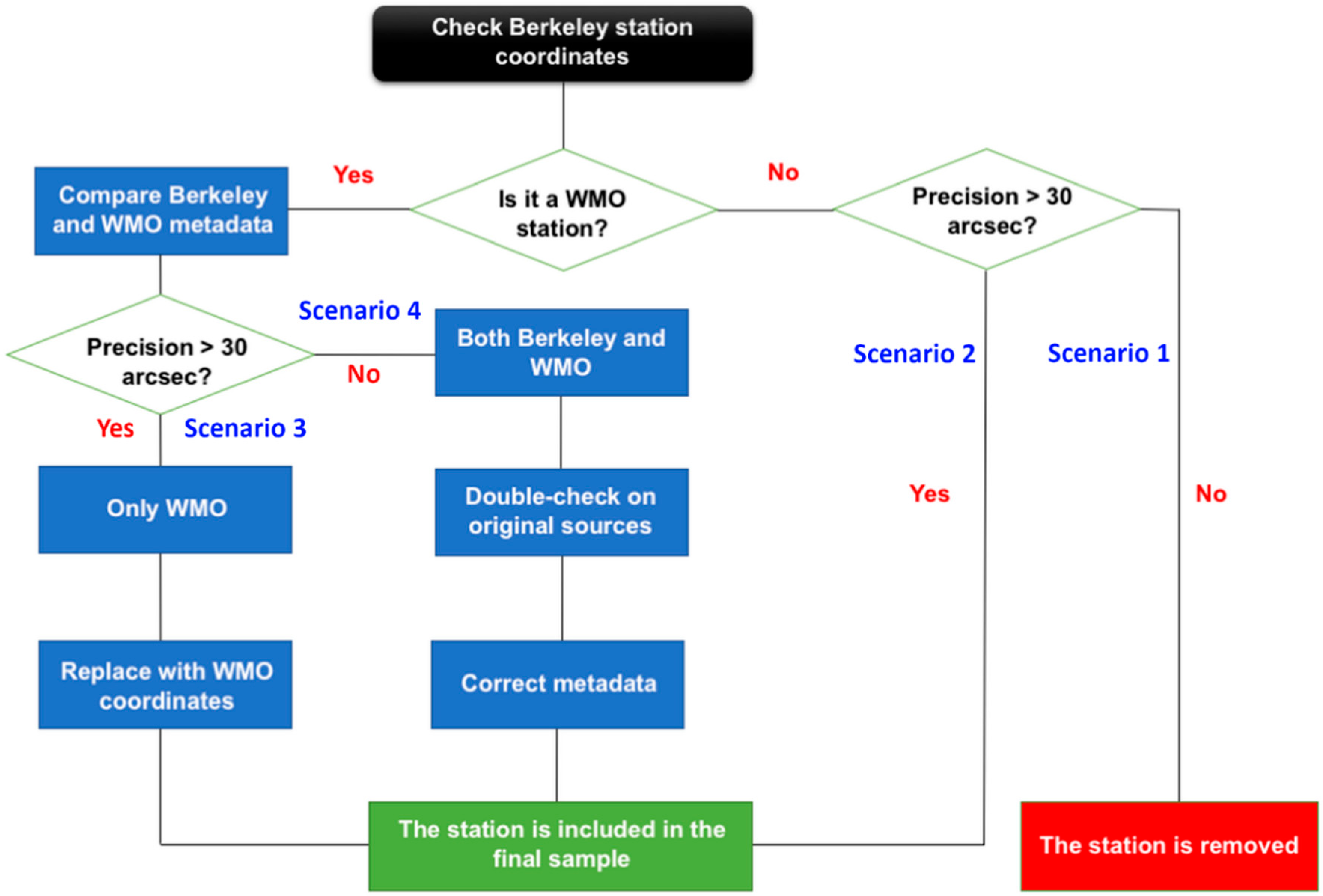
The spatial resolution of temperature data included in the Berkeley Earth dataset is quite heterogeneous, with some stations localized with a 30 arcsec resolution, and others with a lower resolution. This occurs because this dataset includes station data gathered from different sources. To minimize uncertainties, metadata from the Berkeley Earth dataset are compared to official data provided by the WMO weather reports when available [68,69]. WMO weather reports include a full list of all surface and upper-air stations in use at a 30-arcsec resolution (0.00833°) and, thus, provides a precise geo-localization of temperature stations. An iterative statistical-based procedure is performed in order to compare station coordinates in both Berkeley Earth and WMO datasets when available. When inconsistencies in the Berkeley Earth dataset are found, the related coordinates are corrected by using WMO data. Different scenarios could occur. These are described below and we refer to the flowchart in Figure 1 for further details.
- If the weather station from the Berkeley Earth dataset is not available in the WMO list and its spatial resolution is coarser than 30 arcsec, the station is removed.
- If the weather station from the Berkeley Earth dataset is not available in the WMO list and its spatial resolution is equal or more detailed than the 30 arcsec, the station is included in the final sample.
- If the weather station from the Berkeley Earth dataset is included in the WMO list and the spatial resolution provided by the Berkeley Earth dataset is coarser than 30 arcsec, station coordinates are corrected by using those provided by WMO and the station is included in the final sample.
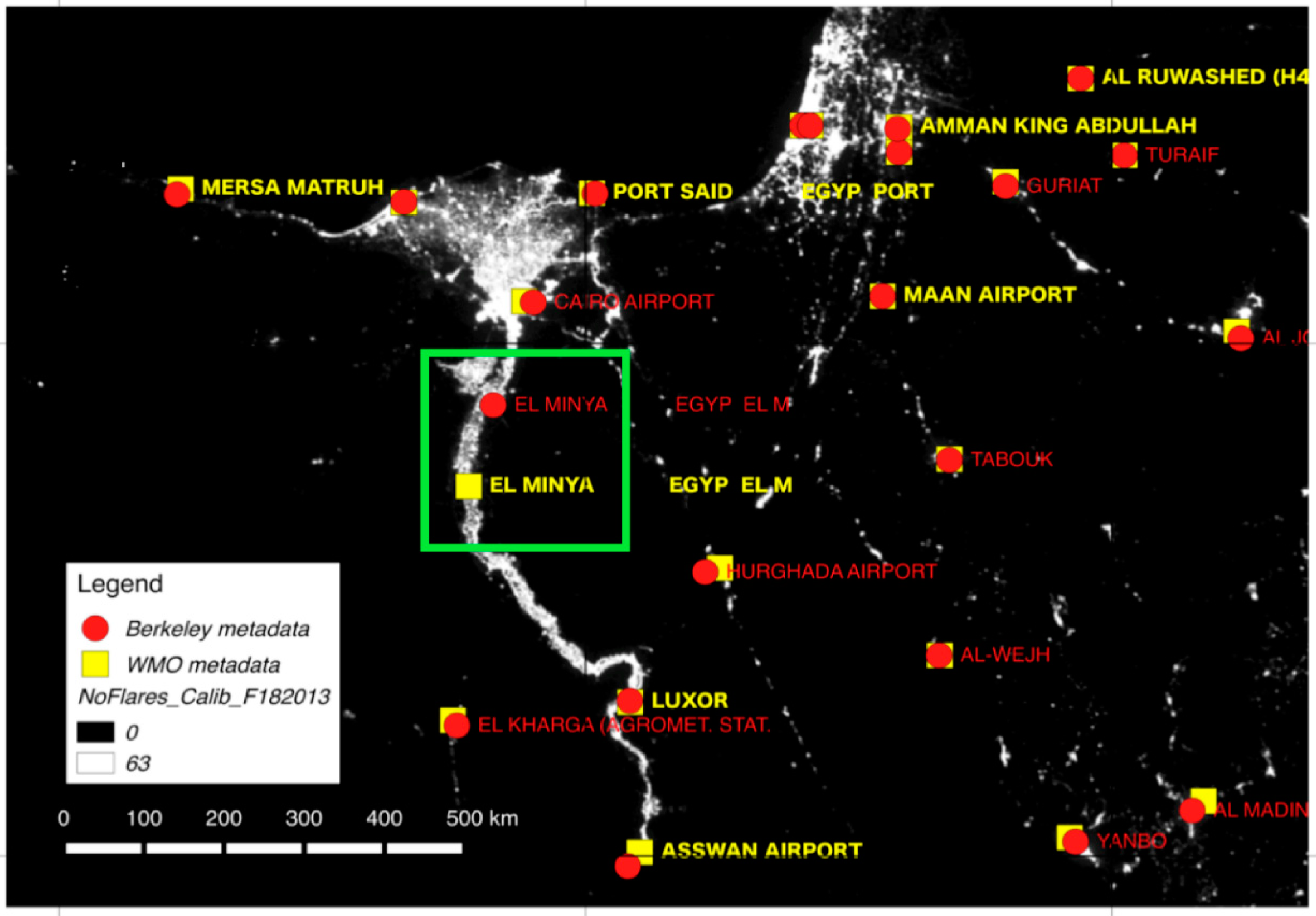
- If the weather station from the Berkeley Earth dataset is included in the WMO list and the spatial resolution provided by the Berkeley Earth dataset is equal or more detailed than 30 arcsec, station coordinates from the two datasets are compared. In case of significant differences (i.e., the station is located in two different grid cells, see Figure 2 as an example), the original sources are consulted to precisely locate the station. Station metadata are, thus, corrected and the station is included in the final sample.
Table S1 in the Supplementary Materials reports the final sample of air temperature stations used in this work, which fulfill the geo-localization procedure (i.e., matching between Berkeley Earth and WMO metadata) [68,69].
3.2. Pairing of Temperature and Nightlights Data
Once the position of the stations has been checked and corrected if necessary, we define a regular square buffer around the pixel where the station is located, which ranges from 3 to 7 pixels (i.e., from 3 to 7 km at the equator approximately). We compute the average annual Digital Number value (L for lights, from now on) for the year i and the station s (Lis) using the equation below.
where Lik is the value in the kth pixel for the year i and ktot is the total number of pixels in the buffer around station s. For example, ktot = 9 in a 3 × 3 km buffer around the station and up to ktot = 49 in a 7 × 7 km buffer. In this regard, indicates that the average is made in 3×3 km buffer, whereas refers to a 7 × 7 km buffer. Buffers smaller than 3 km (i.e., 1 × 1 km and 2 × 2 km) are not considered in order to avoid the spatial noise due to a possible inaccurate geo-localization of air temperature stations. Selected buffers allow one to attenuate this spatial noise (i.e., the local noisy effect is reduced by considering neighboring pixels). The choice of analyzing more than one buffer is due to effects of urban warming that could be detected several kilometers away from the instrument site, even if the major impact is evident in the first kilometer [70].
3.3. Gap-Filling Procedure for Incomplete Time Series of Temperature Records
After having matched temperature and nightlights data, we turn to fill possible gaps in the annual time series of temperature records. The Berkeley Earth dataset provides monthly average data Tij, where i is the year (from 1992 to 2013) and j is the month (from 1 to 12). Yearly data are derived by averaging available monthly data. Since some stations show gaps in monthly data, we apply a statistical procedure to estimate the annual mean temperature in the presence of limited missing data and then fill the gaps (see Text S1 in the Supplementary Materials).
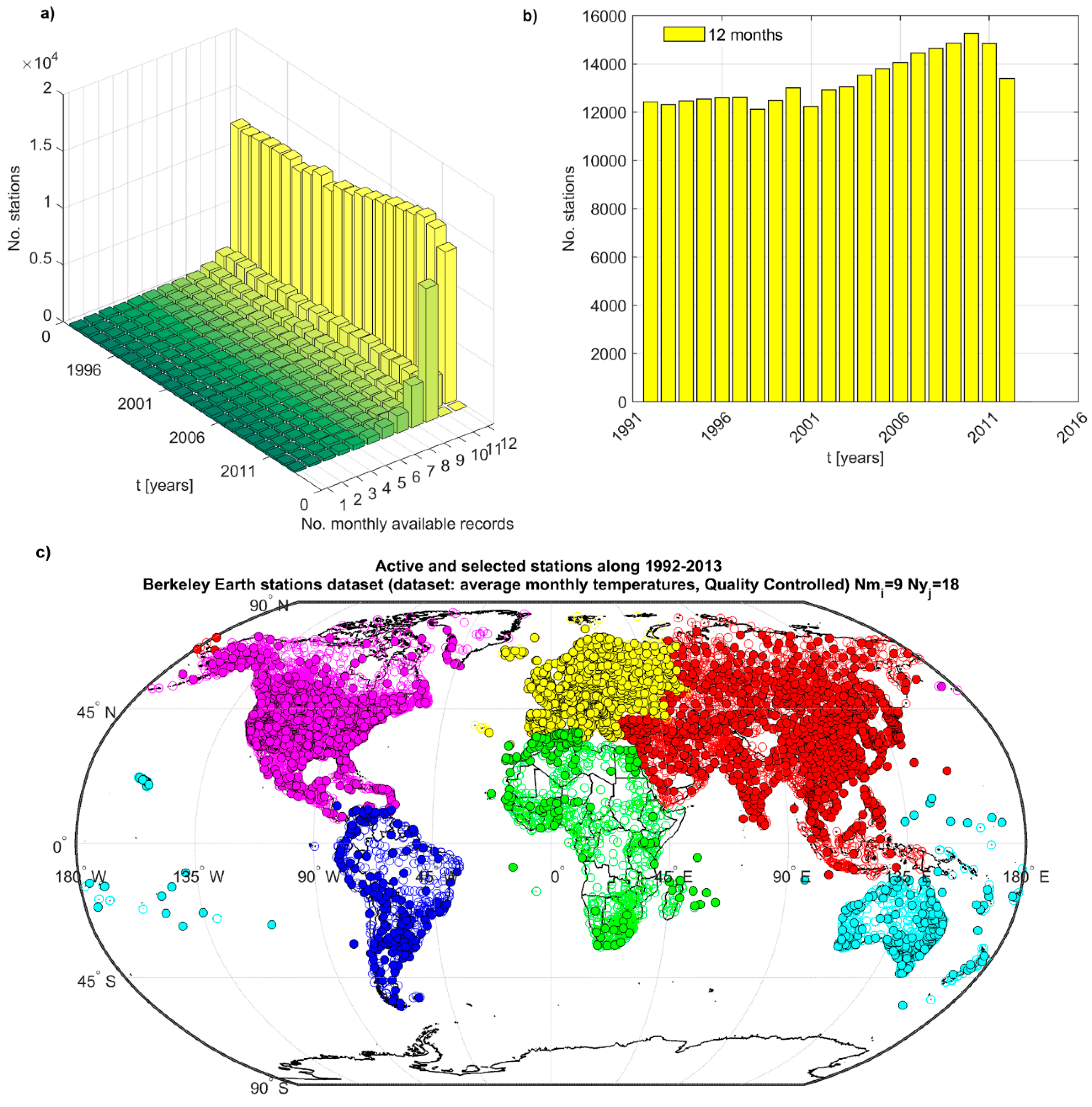
In detail, for a given station s, we call Nmi(s) the number of monthly data available in year i, i = 1992…2013 (0 ≤ Nmi(s) ≤ 12). We also call Nyj(s) the number of available records for month j, j = 1…12 (0 ≤ Nyj(s) ≤ 22). The distribution of Nmi and Nyj values is reported in Figure 3. By performing a sensitivity analysis (see a detailed description of the method and outcomes in S1 Text in the Supplementary Materials), the acceptable number of missing values to perform the gap-filling procedure is identified. The thresholds Nm* = 9 and Ny* = 18 are selected: if Nmi(s) < Nm* (for any i) or Nyj(s) < Ny* (for any j) the air temperature station s is discarded from our analysis. Otherwise, missing data are reconstructed as follows: suppose the temperature observation is missing in station s for month j* in year i*. The reconstructed value is the average of the temperature values available for the same month in other years using the equation below.
where Nyj*(s) is the number of available records for month j* and Tkj*(s) are available temperature data for month j* in year k, k = 1,…,Nyj*(s), respectively. Table S2 in the Supplementary Materials provides an example of application of the performed gap-filling procedure.
Overall, 5530 air temperature stations are selected in this study, meeting both geo-localization and gap-filling requirements (Figure 3c and Table S3 in the Supplementary Materials). The performed data preparation procedure produces a loss of information, from the original 39,000 stations, which show different behaviors across continents. In the case of North America, the loss of information does not significantly influence the analysis, in view of both the high station density and spatial coverage. Conversely, the consistent number of gaps in the temperature datasets in Africa and South America, along with the scarce network coverage, more significantly impacts the consistency of the selected dataset.
4. Methods
In order to investigate the nexus between temperature variations and urbanization trends, as derived from nightlights, a linear regression analysis estimating trends of temperature and nightlights versus time is first performed. A statistical analysis is then proposed to measure the degree of agreement between trends in temperature and nightlights. Results are analyzed on both global and regional (i.e., continental) scales. For the sake of clarity, examples of application are included throughout the text.
4.1. Trend Analysis
Temperature T [°C] and nightlights L [-] trends in the study period from 1992 to 2013 are analyzed through a linear regression model.
For a given station, we fit T values versus time by using the equation below.
where bT identifies the slope of the temperature regression line, aT is the intercept, and t is time. The corresponding linear regression model to fit L values versus time is shown below.
where bL and aL indicate the slope and intercept of the nightlights regression line, respectively.
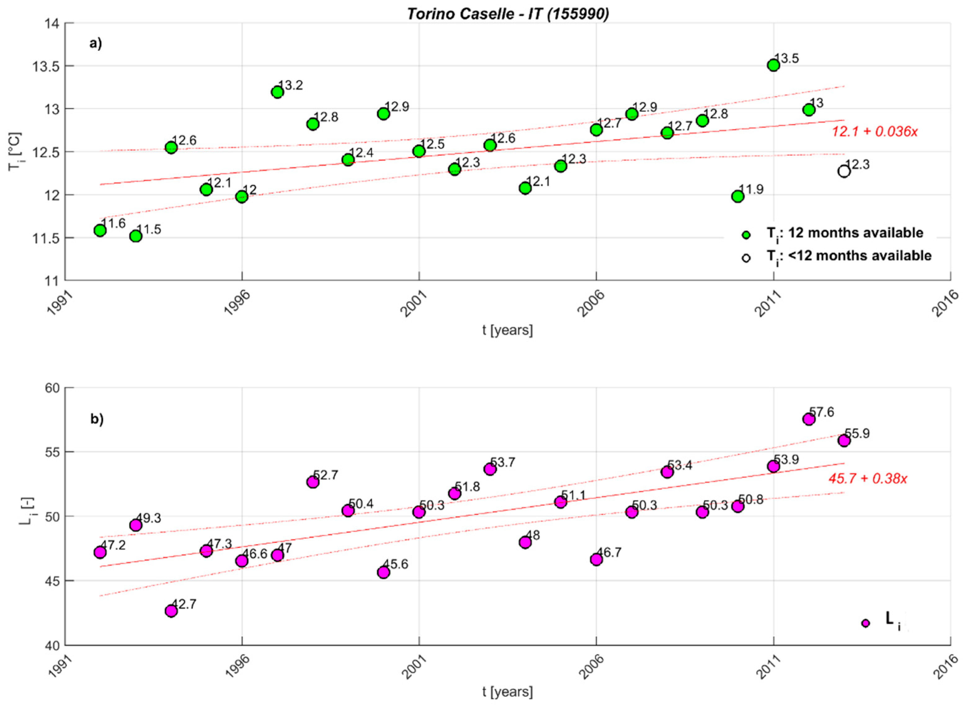
Regression coefficients are estimated via the ordinary least squares method. The slope of the regression line represents the percentage of variation of the temperature (Figure 4a) or the nightlights (Figure 4b) per year.
In order to test the significance of trends, we compute the p-values—pT and pL for temperature and nightlights, respectively—corresponding to the empirically determined slope values on a two-tailed Student’s t distribution with n-2 degrees of freedom, where n = 22 is the sample size, e.g., the length of the observation period in years. The null hypothesis of the test is that there is no trend and we adopt a significance level α = 0.1, i.e., a 0.05 significance level on each tail of the distribution. In the following, we allocate positive significant trends in the class c = 1 (p-value ≥ 0.95), negative significant trends in the class c = 4 (p-value ≤ 0.05), while positive and negative non-significant trends are placed in the classes c = 2 (0.5 < p-value < 0.95) and c = 3 (0.05 < p-value < 0.5), respectively.
Figure 4 shows the application of the linear regression model to a specific station in a 3 × 3 km spatial buffer. In this case, increasing variations in time for both T and L are found, with p-values of the slope regression lines equal to 0.9846 and 0.9998 for temperature and nightlights, respectively. Since both pT and pL are in class 1 (p value ≥ 0.95), this means that significantly positive temperature and nightlight variations occur in the considered buffer.
4.2. Statistical Indicators to Measure the Agreement between Temperature and Nightlights Trends
In order to measure the degree of agreement between the trends of temperature and nightlights, we define an algorithm whose main steps are described below. In the following paragraphs, the results obtained for Asia are used to provide an example of application of the method.
With respect to the considered geographic area (Asia in this case), we compute the percentage of stations with significant (or non-significant) increasing (or decreasing) trends based on related p values. This is performed separately on T and L. We denote these percentages as wTc and wLc, with c = 1,…,4 by using:
where nTc and nLc indicate the number of pT and pL values in the cth class and nTOT the total sample size in the study area. For Asia, nTOT = 1153 (whereas, for the whole globe, nTOT = 5530).
Table 1 shows the percentage of stations in each class of significance c for Asia. For example, 40.8% of stations show a significant and increasing temperature trend and nearly 56% of stations are located in areas of significant increasing luminosity.
We define two variables, denoted as VT and VL, and we assign values to each station and class of significance c: (i) 1 for c = 1, (ii) 0.5 for c = 2 (iii) −0.5 for c = 3, and (iv) −1 for c = 4. Specifically:
The product of VT and VL define the final score assigned to the station. We then compute the expected values of the two variables VT and VL based on the probability of occurrence in class c and value assigned to the stations, which is shown in the equations below.
Likewise, variances are computed using the equation below.
In the case of Asia, the expected values and corresponding variances are E[VT] = 0.42, E[VL] = 0.43, σ2[VT] = 0.42, σ2[VL] = 0.59.
We then define a concordance index CI (which is formally a covariance), which allows one to assess the degree of agreement between the two considered variables VT and VL.
where the product between and represents the contribution of each station to the concordance index. A decreasing index entails a decreasing agreement between pT and pL, which means increasing temperature T (c = 1,2) and decreasing nightlights trends L (c = 3,4) or vice versa. An increasing index is instead associated with increasing agreement. In the case of Asia, CI = 0.22.
If T and L were statistically independent and, therefore, not related, the mean and variance of CI would be computed by using the equation below.
Therefore, Equation (14) provides a reference value to be compared with the CI given by Equation (13) to assess the degree of agreement between T and L. Values of CI can be standardized to make norm-referenced interpretations. We compute a standardized score z using the equation below.
The larger the z value, the more concordant are the variations of temperature and nightlights. Assuming CI is approximately Gaussian-distributed and borrowing some limit values commonly adopted in z-scores interpretation, we have that: if z < −2, T and L variations are strongly discordant. If −2 < z < −1, T and L variations are discordant. If −1 < z < 0, the discordance is weak. If 0 < z < 1, the concordance is weak. If 1 < z < 2, T and L variations are concordant and, if z >2, T and L variations are strongly concordant.
In the case of Asia, we obtain E[CI] = 0.18 σ[CI] = 0.019 and z = 2.1, which has strongly concordant variations in temperature and nightlights.
5. Results
The main outcomes are shown and discussed in the following paragraphs. Hereinafter, we show the results for only the 3 × 3 km buffer. Analyses on larger spatial buffers lead to similar results compared to the 3 × 3 km buffer (see Figures from S1 to S8 in the Supplementary Materials).
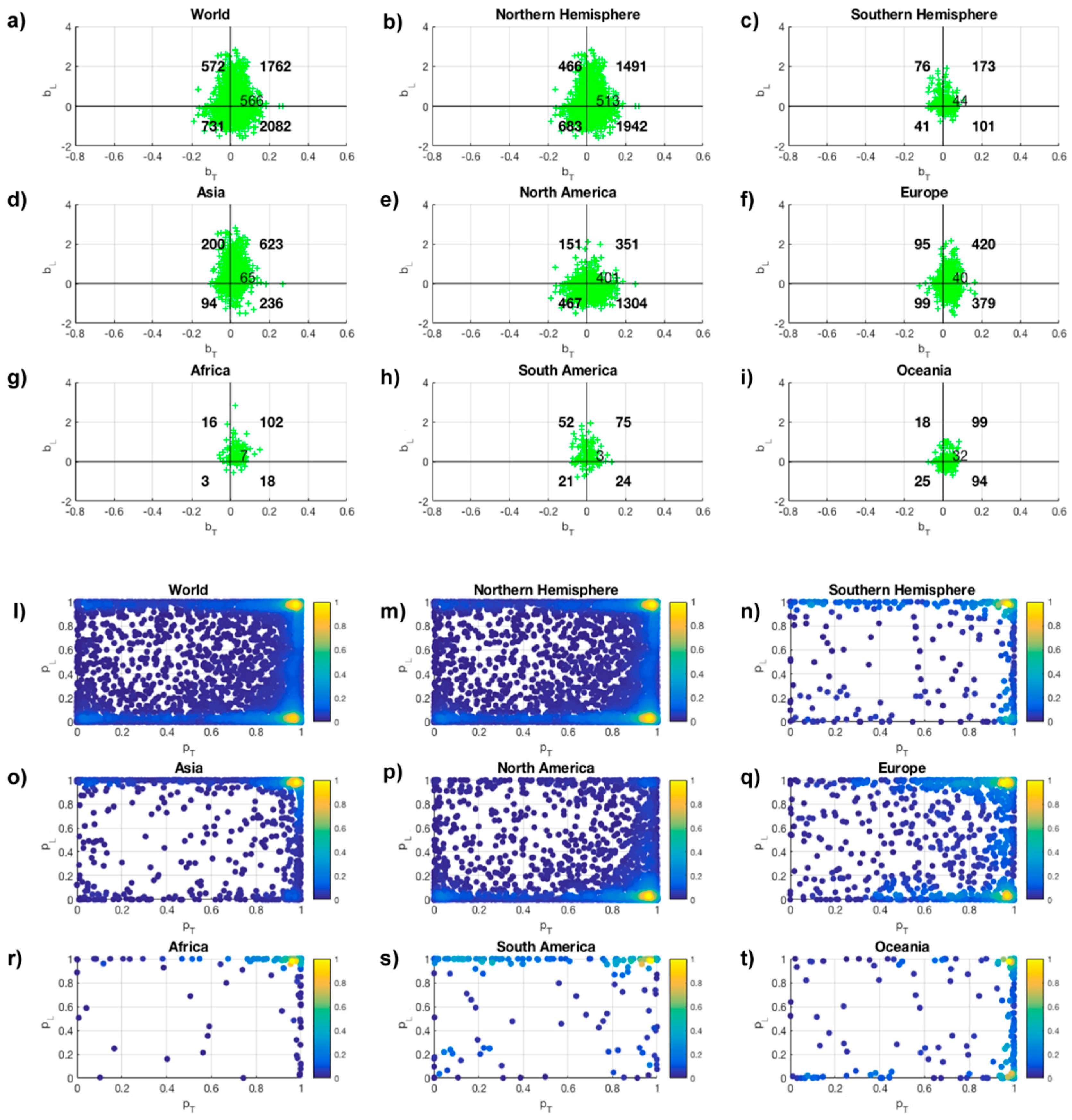
Regression analyses on mean annual T and L are carried out for each station as outlined in the Methods section. Results are reported in Figure 5a–i, where the slopes of T and L regression lines are reported. Sectors 1 and 3 represent positive and negative concordant trends, while sectors 2 and 4 refer to discordant trends, e.g., a rise in temperature in correspondence of a decreasing nightlights trend (sector 4) and vice versa (sector 2). Interesting differences emerge at the continental scale. A positive agreement is detected in more than 50%, 69%, and 43% of stations in Asia, Africa, and South America. In those regions, most stations are located in more and more anthropized areas and experienced an increase of temperature in the period from 1992 to 2013. A unique pattern can be noticed in South America, where 30% of stations are located in areas with increasing nightlights but decreasing temperature trends. In Europe, concordant and discordant patterns are almost balanced. In Oceania, most stations are experiencing warming i.e., more than 70% out of the total, with both increasing (37%) and decreasing (35%) nightlight trends. More than 62% of North American stations show negative luminosity tendency (mostly due to measures to reduce light pollution) in more than 49% of the cases in conjunction with warming trends. This tendency is reflected in the Northern Hemisphere and worldwide due to the large number of stations located in the USA.
Figure 6 summarizes the outcomes from our algorithm to assess the concordance between trends of different variables. As the first outcome, the majority of air temperature stations is experiencing warming trends: pT for more than 70% of the selected stations is in class c equal to 1 and 2 (wT1, wT2), with the sole exception of South America (Figure 6f), where negative and positive temperature trends are almost balanced. The global distribution of L is clearly bimodal, with two peaks in class 1 and class 4 (the latter are mostly related to stations in North America).
The computation of the concordance index CI (Equation (13)) reveals an appreciable degree of concordance between T and L trends in Asia and Europe and a weak positive concordance in Africa, South America, and Oceania. The discordance detected in North America moves the CI toward a negative value on a global scale (Figure 6a,h). The standardized z scores, thus, move in the direction of an overall tendency toward positive concordance, except for North America.
6. Discussion and Conclusions
In this work, we introduce a new way of quantifying the nexus between the evolution in time of thermal impacts and urbanization at multiple scales. Our results confirm the overall tendency of urbanization trends to affect temperature changes. A significant increment of temperature in concomitance with increasing luminosity variations are detected worldwide, and regional-scale results are generally in agreement with this overall trend.
We quantitatively assess the degree of agreement across the four different classes of trend significance using a statistical indicator, which computes the percentage of stations included in each class of significance, based on temperature and nightlights trends. The majority of stations are experiencing warming trends since pT values are mainly included in the first two classes (wT1, wT2).
Recent studies at a very local scale show that the size of the source radius (i.e., buffer) matters when assessing urban influences on station temperature trends, and the near-station surroundings have been demonstrated to be more influential for temperature values [52]. Nevertheless, analyses with larger spatial buffers tend to confirm the patterns detected in the 3 × 3 km buffer (Figures S1–S8 in the Supplementary Materials). Cities expand toward neighboring non-urbanized areas, which cause their edges to become brighter [71]. This shows that (i) anthropogenic pressure still grows towards new and peripheric areas, and (ii) most parts of the suburbs continue to experience warming relative to nearby rural sites [70].
As confirmed by recent findings at the regional scale in Italy, with urban dispersion, peri-urban areas become progressively more and more vulnerable to climate change [72]. Besides the background climate, urban landscape morphology likely plays a major role in shaping the spatial variability of urbanization-induced warming such as for some Chinese regions [27]. From an urban extent point of view, results on a number of European cities confirm that UHI in an urban sprawl, stretched and polycentric cities is less intense [36]. Not only urban expansion, but variation in density within cities is another relevant issue to be further addressed in the future [73].
The analyses on the agreement of temperatures and luminosity variations on a continental scale could provide interesting insights into the sociodemographic and economic features of single continents. For instance, Africa and Asia reveal significant increasing temperature trends along with nightlight increments in recent years, which reflect the fast-evolving and uncontrolled urbanization in these areas. In such areas, recent studies highlight that urban land expansion is explained by different factors. For example, China’s urban land expansion is driven more by economic rise than population while, in India, population growth drives urban land sprawl [74]. Most urban growth around the world, and especially in middle-income and low-income continents such as Africa and Asia, is taking place on prime agricultural land [75]. By being less urbanized, region-specific projections reveal that these areas are expected to experience relatively faster rates of urbanization over the next 30 years [76,77].
Increasing temperatures along with slightly positive or negative nightlight trends mainly correspond to developed continents. It is worth noting that developed countries have already experienced major urbanization expansion in past decades. In such context, the heating effect due to urban sprawl tends to flatten with the increase of urban areas beyond a certain size because the increase in the density of the urban built environment and activities is not infinite [18,20]. As cities grow, temperatures in pre-existing urban areas in some cases are pretty stable, while temperatures only rise in newly urbanized areas [78]. This is confirmed by recent studies showing that, when temperatures rise in pre-existing urban areas, the air temperature change is smaller than newly urbanized ones [79]. Moreover, based on UN projections [9] and other studies, the urban population in some cities across Europe is expected to decline by 2050 [9,76,77].
The significant decrement of night time luminosity detected in North America could be the result of policy-driven initiatives as light pollution abatement programs promoted in these last years in western countries such as in Canada and in at least 18 U.S. states [55,71,80,81]. The same initiative has been undertaken in many countries in Northern Europe such as the United Kingdom and the Netherlands [59,62]. This makes the interpretation of urbanization dynamics more complex on temperature trends. In locations such as North America and parts of Europe, the mere use of nightlights as a proxy of urbanization may lead to the misleading conclusion that T increases independently of the entity of urbanization, which suggests a minimum UHI effect in regional warming. Nevertheless, this is not confirmed by regional analyses worldwide, where the increment of urbanization seems to be of value in explaining temperature variations [28]. Therefore, in such cases, contingent regionally-based studies are crucial in solving the issue [27,28]. Regionally-based studies could reveal more about the importance of scale-dependency of the nexus between climate patterns and urbanization [20,27]. Studies on cities across North America reveal that the local background climate greatly contributes to UHI [82] and that temperature trends differ between northern and southern latitudes because of biomes [20]. Relevant urbanization patterns exist in Europe that can be captured by nightlights and recent studies confirm that there is a strong variation of urbanization dynamics within single countries and regions, which is in line with our findings [66]. Subnational levels of analysis in Europe reveal that changes in nightlights luminosity are influenced by a number of drivers e.g., the socioeconomic context and national and regional policies [66]. Preliminary work reveal that, when analyses on Central-Northern and Southern countries are performed separately, the Mediterranean area countries reveal a clear tendency toward a significant positive concordance, while other factors, such as light pollution abatement programs, could be responsible for the discordance detected in Northern Europe [83]. On the other hand, cooler Northern European cities appear to be more vulnerable to UHI effects than Southern cities, which appear to be well-adapted [84]. These studies, along with our findings, stress the importance of mutual relations and feedbacks between regional warming and urbanization dynamics. Decreasing temperature trends detected in South America could be related to mesoscale effects (i.e., related to meteorological phenomena from approximately 10 to 1000 km in a horizontal extent such as between a microscale and synoptic scale). Recent findings outline that the intensification of the South Pacific Anticyclone during these last years, which is a consequence of global warming, could contribute to the coastal cooling and warming in the continental Chile and Andes [85,86]. Other previous studies show that, in the past, there has been net cooling over Argentina (about −0.04 °C/decade) in contrast to other land areas. This occurs mainly in the areas where precipitation has increased the most likely due to an increase in the moisture transport from the Amazon to Northern Argentina by the low-level jet [87]. Nightlights trends in South America are growing with a slower rate than in Asia and Africa. South America is more urbanized than these regions since the level of urbanization was around 81%, which matches that of North America (82%) as well as many European countries (68%) [9]. Consequently, the rate of urbanization in South America is quite slow compared to other developing regions, as confirmed by previous studies and projections [76].
Although satellite data provide information that is not directly related to the quantitative rise of temperature records, in this work, we prove how these data can support both global and local analyses of urban and global warming-related issues. Our analysis performed over a wide range of spatial scales presents some uncertainty associated with the reliability of urban temperature records, which provides the ground for future discussion on the effect of urban heating on climate data. Further advances in this direction could benefit from the perspectives offered by new approaches and techniques, and from further studies showcasing the multi-scale impacts of urbanization on the climate. Merging high-resolution data as nightlights, which was made available by new advances in remote-sensing, statistical models, and concepts, could represent the opportunity for an unconventional strategy to analyze such issues.
Supplementary Materials
The following are available online at https://www.mdpi.com/2073-4433/10/3/117/s1, Text S1: Reconstruction procedure in annual average temperature data. Table S1: Matching between the final sample of Berkeley Earth and official WMO stations used in this work (5530 stations). Stations are provided with related ID codes, coordinates, and precision. In the case of WMO stations, the precision of the coordinates is not reported since the minimum resolution is always equal or higher than 30 arcsec. When no matching with the WMO station is available, WMO coordinates are denoted as “NaN”. Table S2: Table. Example of application of a reconstruction procedure of annual average temperature. In the selected station Torino Caselle (Berkeley ID 155990) two gaps in November and December 2013 (i = 22) are found. Table S3: Active and selected air temperature stations in the study period from 1992 to 2013 for “Quality Controlled” data derived from the Berkeley Earth dataset. Number of active (i.e., having at least one year of data) stations from 1992 to 2013 and available stations after the application of thresholds for the reconstruction of mean annual temperature from the mean monthly data and spatial localization. The selected thresholds are Nmi ≥ 9 and Nyj ≥ 18. The percentages refer to the total sample of active and selected stations respectively. Figure S1: Slope of T (bT) and L (bL) regression trend lines at a global and continental scale, 4 × 4 km buffer. Sectors 1 and 3 correspond to agreeing trends while sectors 2 and 4 refer to discordant trends. The number of stations included in each sector is in bold as well as the number of stations with L systematically equal to zero (bL = 0) on the horizontal axis. Figure S2: P values density plots at a global and continental scale, 4x4 km buffer. The color scale represents the data density. Figure S3: Slope of T (bT) and L (bL) regression trend lines on a global and continental scale, 5 × 5 km buffer. Sectors 1 and 3 correspond to agreeing trends while sectors 2 and 4 refer to discordant trends. The number of stations included in each sector is in bold as well as the number of stations with L systematically equal to zero (bL = 0) on the horizontal axis. Figure S4: P values density plots at global and continental scales, 5 × 5 km buffer. The color scale represents the data density. Figure S5: Slope of T (bT) and L (bL) regression trend lines at a global and continental scale. 6 × 6 km buffer. Sectors 1 and 3 correspond to agreeing trends, while sectors 2 and 4 refer to discordant trends. The number of stations included in each sector is in bold, as well as the number of stations with L systematically equal to zero (bL = 0) on the horizontal axis. Figure S6: P values density plots at a global and continental scale. 6 × 6 km buffer. The color scale represents the data density. Figure S7: Slope of T (bT) and L (bL) regression trend lines at a global and continental scale. 7 × 7 km buffer. Sectors 1 and 3 correspond to agreeing trends, while sectors 2 and 4 refer to discordant trends. The number of stations included in each sector is in bold, as well as the number of stations with L systematically equal to zero (bL = 0) on the horizontal axis., Figure S8: P values density plots at a global and continental scale, 7 × 7 km buffer. The color scale represents the data density.
Author Contributions
R.P. and S.C. collected and processed all data. F.L. and A.M. supervised the research. All authors conceived the methodology and wrote the manuscript.
Funding
F.L. and R.P. acknowledge support from the ERC project CoG 647473. S.C. and A.M. acknowledge the support of the Italian Ministry of Education, Universities, and Research through the grant “Department of Excellence 2018-2022” awarded to the Department DICAM at the University of Bologna.
Conflicts of Interest
The authors declare no conflict of interest.
References
- Dodman, D. International Encyclopedia of Geography: People, the Earth, Environment and Technology; Environment and Urbanization: Thousand Oaks, CA, USA, 2017; pp. 1–9. ISBN 978-0-470-65963-2. [Google Scholar]
- IPCC. Part A: Global and Sectoral Aspects. (Contribution of Working Group II to the Fifth Assessment Report of the Intergovernmental Panel on Climate Change). In Climate Change 2014–Impacts, Adaptation and Vulnerability; IPCC: Geneva, Switzerland, 2014. [Google Scholar]
- Zhou, Y.; Smith, S.J.; Zhao, K.; Imhoff, M.; Thomson, A.; Bond-Lamberty, B.; Asrar, G.R.; Zhang, X.; He, C.; Elvidge, C.D. A global map of urban extent from nightlights. Environ. Res. Lett. 2015, 10, 054011. [Google Scholar] [CrossRef] [Green Version]
- Santamouris, M.; Cartalis, C.; Synnefa, A.; Kolokotsa, D. On the impact of urban heat island and global warming on the power demand and electricity consumption of buildings—A review. Energy Build. 2015, 98, 119–124. [Google Scholar] [CrossRef]
- Peng, S.; Piao, S.; Ciais, P.; Friedlingstein, P.; Ottle, C.; Bréon, F.M.; Nan, H.; Zhou, L.; Myneni, R.B. Surface urban heat island across 419 global big cities. Environ. Sci. Technol. 2012, 46, 696–703. [Google Scholar] [CrossRef] [PubMed]
- Vörösmarty, C.J.; Green, P.; Salisbury, J.; Lammers, R.B. Global water resources: Vulnerability from climate change and population growth. Science 2000, 289, 284–288. [Google Scholar] [CrossRef] [PubMed]
- Jones, G.A.; Warner, K.J. The 21st century population-energy-climate nexus. Energy Policy 2016, 93, 206–212. [Google Scholar] [CrossRef]
- Kovats, S.; Akhtar, R. Climate, climate change and human health in Asian cities. Environ. Urban. 2008, 20, 165–175. [Google Scholar] [CrossRef] [Green Version]
- UN DESA. World Urbanization Prospects: The 2018 Revision; United Nations: New York City, NY, USA, 2018. [Google Scholar]
- Kalnay, E.; Cai, M. Impact of urbanization and land-use change on climate. Nature 2003, 423, 528–531. [Google Scholar] [CrossRef] [PubMed]
- Hansen, J.; Ruedy, R.; Sato, M.; Lo, K. Global surface temperature change. Rev. Geophys. 2010, 48, RG4004. [Google Scholar] [CrossRef]
- McCarthy, M.P.; Best, M.J.; Betts, R.A. Climate change in cities due to global warming and urban effects. Geophys. Res. Lett. 2010, 37, 1–5. [Google Scholar] [CrossRef]
- Parker, D.E. Urban heat island effects on estimates of observed climate change. Wiley Interdiscip. Rev. Clim. Chang. 2010, 1, 123–133. [Google Scholar] [CrossRef]
- Hausfather, Z.; Menne, M.J.; Williams, C.N.; Masters, T.; Broberg, R.; Jones, D. Quantifying the effect of urbanization on u.s. Historical climatology network temperature records. J. Geophys. Res. Atmos. 2013, 118, 481–494. [Google Scholar] [CrossRef]
- Wickham, C.; Rohde, R.; Muller, R.A.; Wurtele, J.; Curry, J.; Groom, D.; Jacobsen, R.; Perlmutter, S.; Rosenfeld, A.; Mosher, S. Influence of Urban Heating on the Global Temperature Land Average using Rural Sites Identified from MODIS Classifications. Geoinform. Geostatist. 2013, 1, 1–6. [Google Scholar]
- Arnfield, A.J. Two decades of urban climate research: A review of turbulence, exchanges of energy and water, and the urban heat island. Int. J. Climatol. 2003, 23, 1–26. [Google Scholar] [CrossRef]
- Jones, P.D.; Groisman, P.Y.; Coughlan, M.; Plummer, N.; Wang, W.C.; Karl, T.R. Assessment of urbanization effects in time series of surface air temperature over land. Nature 1990, 347, 169–172. [Google Scholar] [CrossRef]
- Oke, T.R. The energetic basis of the urban heat island. Q. J. R. Meteorol. Soc. 1982, 108, 1–24. [Google Scholar] [CrossRef]
- Creutzig, F. Towards typologies of urban climate and global environmental change. Environ. Res. Lett. 2015, 10. [Google Scholar] [CrossRef]
- Li, X.; Zhou, Y.; Asrar, G.R.; Imhoff, M.; Li, X. The surface urban heat island response to urban expansion: A panel analysis for the conterminous United States. Sci. Total Environ. 2017, 605–606, 426–435. [Google Scholar] [CrossRef] [PubMed]
- Chapman, S.; Watson, J.E.M.; Salazar, A.; Thatcher, M.; McAlpine, C.A. The impact of urbanization and climate change on urban temperatures: A systematic review. Landsc. Ecol. 2017, 32, 1921–1935. [Google Scholar] [CrossRef]
- Pielke, R.A.; Matsui, T. Should light wind and windy nights have the same temperature trends at individual levels even if the boundary layer averaged heat content change is the same? Geophys. Res. Lett. 2005, 32, L21813. [Google Scholar] [CrossRef]
- Akbari, H.; Bell, R.; Brazel, T.; Cole, D.; Estes, M.; Heisler, G.; Hitchcock, D.; Johnson, B.; Lewis, M.; McPherson, G.; et al. Reducing Urban Heat Islands: Compendium of Strategies—Urban Heat Island Basics; Environmental Protection Agency: Washington, DC, USA, 2008; pp. 1–22.
- Santamouris, M. Energy and Climate in the Urban Built Environment; Routledge: Abingdon, UK, 2013; ISBN 9781315073774. [Google Scholar]
- Voogt, J.; Oke, T. Thermal remote sensing of urban climates. Remote Sens. Environ. 2003, 86, 370–384. [Google Scholar] [CrossRef]
- Imhoff, M.L.; Zhang, P.; Wolfe, R.E.; Bounoua, L. Remote sensing of the urban heat island effect across biomes in the continental USA. Remote Sens. Environ. 2010, 114, 504–513. [Google Scholar] [CrossRef] [Green Version]
- Cao, Q.; Yu, D.; Georgescu, M.; Wu, J. Impacts of urbanization on summer climate in China: An assessment with coupled land-atmospheric modeling. J. Geophys. Res. 2016, 121, 10,505–10,521. [Google Scholar] [CrossRef]
- Georgescu, M.; Morefield, P.E.; Bierwagen, B.G.; Weaver, C.P. Urban adaptation can roll back warming of emerging megapolitan regions. Proc. Natl. Acad. Sci. USA 2014, 111, 2909–2914. [Google Scholar] [CrossRef] [PubMed] [Green Version]
- Krayenhoff, E.S.; Moustaoui, M.; Broadbent, A.M.; Gupta, V.; Georgescu, M. Diurnal interaction between urban expansion, climate change and adaptation in US cities. Nat. Clim. Chang. 2018, 8, 1097–1103. [Google Scholar] [CrossRef]
- Debbage, N.; Shepherd, J.M. The urban heat island effect and city contiguity. Comput. Environ. Urban Syst. 2015, 54, 181–194. [Google Scholar] [CrossRef]
- Chen, X.; Nordhaus, W.D. Using luminosity data as a proxy for economic statistics. Proc. Natl. Acad. Sci. USA 2011, 108, 8589–8594. [Google Scholar] [CrossRef] [PubMed] [Green Version]
- Chand, T.R.K.; Badarinath, K.V.S.; Elvidge, C.D.; Tuttle, B.T. Spatial characterization of electrical power consumption patterns over India using temporal DMSP-OLS night-time satellite data. Int. J. Remote Sens. 2009, 30, 647–661. [Google Scholar] [CrossRef]
- Bounoua, L.; Zhang, P.; Mostovoy, G.; Thome, K.; Masek, J.; Imhoff, M.; Shepherd, M.; Quattrochi, D.; Santanello, J.; Silva, J.; et al. Impact of urbanization on US surface climate. Environ. Res. Lett. 2015, 10, 084010. [Google Scholar] [CrossRef] [Green Version]
- Stone Jr., B. Short Communication Urban and rural temperature trends in proximity to large US cities: 1951–2000. Int. J. Clim. A J. R. Meteorol. Soc. 2007, 1807, 1801–1807. [Google Scholar]
- Emadodin, I.; Taravat, A.; Rajaei, M. Effects of urban sprawl on local climate: A case study, north central Iran. Urban Clim. 2016, 17, 230–247. [Google Scholar] [CrossRef]
- Zhou, B.; Rybski, D.; Kropp, J.P. The role of city size and urban form in the surface urban heat island. Sci. Rep. 2017, 7, 1–9. [Google Scholar] [CrossRef] [PubMed]
- Georgiadis, T. Urban Climate and Risk. Oxford Handbooks Online; Oxford University Press: Oxford, UK, 2017; pp. 1–29. [Google Scholar] [CrossRef]
- Kassomenos, P.A.; Katsoulis, B.D. Mesoscale and macroscale aspects of the morning Urban Heat Island around Athens, Greece. Meteorol. Atmos. Phys. 2006, 94, 209–218. [Google Scholar] [CrossRef]
- Yang, X.; Ruby Leung, L.; Zhao, N.; Zhao, C.; Qian, Y.; Hu, K.; Liu, X.; Chen, B. Contribution of urbanization to the increase of extreme heat events in an urban agglomeration in east China. Geophys. Res. Lett. 2017, 44, 6940–6950. [Google Scholar] [CrossRef]
- Zhou, L.; Dickinson, R.E.; Tian, Y.; Fang, J.; Li, Q.; Kaufmann, R.K.; Tucker, C.J.; Myneni, R.B. Evidence for a significant urbanization effect on climate in China. Proc. Natl. Acad. Sci. USA 2004, 101, 9540–9544. [Google Scholar] [CrossRef] [PubMed] [Green Version]
- NASA EOSDIS Land Processes DAAC MCD12Q1 V006|LP DAAC: NASA Land Data Products and Services. Available online: https://lpdaac.usgs.gov/dataset_discovery/modis/modis_products_table/mcd12q1_v006 (accessed on 16 January 2019).
- Vancutsem, C.; Ceccato, P.; Dinku, T.; Connor, S.J. Evaluation of MODIS land surface temperature data to estimate air temperature in different ecosystems over Africa. Remote Sens. Environ. 2010, 114, 449–465. [Google Scholar] [CrossRef]
- Schneider, A.; Friedl, M.A.; Potere, D. Mapping global urban areas using MODIS 500-m data: New methods and datasets based on “urban ecoregions”. Remote Sens. Environ. 2010, 114, 1733–1746. [Google Scholar] [CrossRef]
- Friedl, M.; McIver, D.; Hodges, J.C.; Zhang, X.; Muchoney, D.; Strahler, A.; Woodcock, C.; Gopal, S.; Schneider, A.; Cooper, A.; et al. Global land cover mapping from MODIS: Algorithms and early results. Remote Sens. Environ. 2002, 83, 287–302. [Google Scholar] [CrossRef]
- Fu, P.; Weng, Q. A time series analysis of urbanization induced land use and land cover change and its impact on land surface temperature with Landsat imagery. Remote Sens. Environ. 2016, 175, 205–214. [Google Scholar] [CrossRef]
- Small, C.; Elvidge, C.D.; Balk, D.; Montgomery, M. Spatial scaling of stable night lights. Remote Sens. Environ. 2011, 115, 269–280. [Google Scholar] [CrossRef]
- Marconcini, M.; Metz, A.; Esch, T.; Zeidler, J. Global Urban Growth Monitoring by Means of Sar Data. In Proceedings of the 2014 IEEE Geoscience and Remote Sensing Symposium, Quebec City, QC, Canada, 13–18 July 2014; pp. 1477–1480. [Google Scholar]
- Zhang, P.; Imhoff, M.L.; Wolfe, R.E.; Bounoua, L. Characterizing Urban Heat Islands of Global Settlements Using MODIS and Nighttime Lights Products. Can. J. Remote Sens. J. Can. Teledetect. 2010, 36, 185–196. [Google Scholar] [CrossRef]
- Arino, O.; Gross, D.; Ranera, F.; Leroy, M.; Bicheron, P.; Brockman, C.; Defourny, P.; Vancutsem, C.; Achard, F.; Durieux, L.; et al. GlobCover: ESA service for global land cover from MERIS. In Proceedings of the 2007 IEEE International Geoscience and Remote Sensing Symposium, Barcelona, Spain, 23–28 July 2007; pp. 2412–2415. [Google Scholar]
- Bartholomé, E.; Belward, A.S. GLC2000: A new approach to global land cover mapping from Earth observation data. Int. J. Remote Sens. 2005, 26, 1959–1977. [Google Scholar] [CrossRef]
- Bagan, H.; Yamagata, Y. Analysis of urban growth and estimating population density using satellite images of nighttime lights and land-use and population data. GIScience Remote Sens. 2015, 52, 765–780. [Google Scholar] [CrossRef]
- Lindén, J.; Esper, J.; Holmer, B. Using land cover, population, and night light data for assessing local temperature differences in Mainz, Germany. J. Appl. Meteorol. Climatol. 2015, 54, 658–670. [Google Scholar] [CrossRef]
- Peterson, T.C.; Owen, T.W.; Nesdis, N.; Climatic, N.; Carolina, N. Urban Heat Island Assessment: Metadata Are Important. J. Clim. 2005, 18, 2637–2646. [Google Scholar] [CrossRef]
- Wardrop, N.A.; Jochem, W.C.; Bird, T.J.; Chamberlain, H.R.; Clarke, D.; Kerr, D.; Bengtsson, L.; Juran, S.; Seaman, V.; Tatem, A.J. Spatially disaggregated population estimates in the absence of national population and housing census data. Proc. Natl. Acad. Sci. USA 2018, 115, 201715305. [Google Scholar] [CrossRef] [PubMed]
- Cauwels, P.; Pestalozzi, N.; Sornette, D. Dynamics and spatial distribution of global nighttime lights. EPJ Data Sci. 2014, 3. [Google Scholar] [CrossRef] [Green Version]
- Imhoff, M.L.; Lawrence, W.T.; Stutzer, D.C.; Elvidge, C.D. A technique for using composite DMSP/OLS “city lights” satellite data to map urban area. Remote Sens. Environ. 1997, 61, 361–370. [Google Scholar] [CrossRef]
- Elvidges, C.; Suttonb, P.; Ghoshc, T.; Tuttlec, B.T.; Baughc, K.E.; Bhadurid, B.; Brightd, E.; Elvidgea, C.D.; Sutton, P.C.; Ghoshc, T.; et al. A global poverty map derived from satellite data. Comput. Geosci. 2009, 35, 1652–1660. [Google Scholar] [CrossRef]
- Small, C.; Pozzi, F.; Elvidge, C.D. Spatial analysis of global urban extent from DMSP-OLS night lights. Remote Sens. Environ. 2005, 96, 277–291. [Google Scholar] [CrossRef]
- Bennie, J.; Davies, T.W.; Duffy, J.P.; Inger, R.; Gaston, K.J. Contrasting trends in light pollution observed night time lights. Nature 2014, 4, 1–6. [Google Scholar]
- Ceola, S.; Laio, F.; Montanari, A. Satellite nighttime lights reveal increasing human exposure to floods worldwide. Geophys. Res. Lett. 2014, 41, 7184–7190. [Google Scholar] [CrossRef] [Green Version]
- Soto Gómez, A.J.; Di Baldassarre, G.; Rodhe, A.; Pohjola, V.A. Remotely sensed nightlights to map societal exposure to hydrometeorological hazards. Remote Sens. 2015, 7, 12380–12399. [Google Scholar] [CrossRef]
- Ceola, S.; Laio, F.; Montanari, A. Human-impacted waters: New perspectives from global high-resolution monitoring. Water Resour. Res. 2015, 51, 7064–7079. [Google Scholar] [CrossRef] [Green Version]
- NOAA Earth Observation Group—Defense Meteorological Satellite Progam, Boulder|ngdc.noaa.gov. Available online: https://ngdc.noaa.gov/eog/dmsp/downloadV4composites.html (accessed on 13 December 2018).
- Huang, Q.; Yang, X.; Gao, B.; Yang, Y.; Zhao, Y. Application of DMSP/OLS nighttime light images: A meta-analysis and a systematic literature review. Remote Sens. 2014, 6, 6844–6866. [Google Scholar] [CrossRef]
- Goldblatt, R.; Stuhlmacher, M.F.; Tellman, B.; Clinton, N.; Hanson, G.; Georgescu, M.; Wang, C.; Serrano-Candela, F.; Khandelwal, A.K.; Cheng, W.H.; et al. Using Landsat and nighttime lights for supervised pixel-based image classification of urban land cover. Remote Sens. Environ. 2018, 205, 253–275. [Google Scholar] [CrossRef]
- Stathakis, D.; Tselios, V.; Faraslis, I. Urbanization in European regions based on night lights. Remote Sens. Appl. Soc. Environ. 2015, 2, 26–34. [Google Scholar] [CrossRef]
- Berkeley Earth Berkeley Earth. Available online: http://berkeleyearth.org/about-data-set/ (accessed on 4 October 2017).
- WMO OSCAR Observing Systems Capability Analysis and Review Tool. Available online: https://oscar.wmo.int/surface//index.html#/ (accessed on 15 January 2019).
- WMO. Weather Reporting, Observing Stations; WMO: Geneva, Switzerland, 2014; p. 602. [Google Scholar]
- Nel·lo, O.; López, J.; Martín, J.; Checa, J. Energy and urban form. The growth of European cities on the basis of night-time brightness. Land Use Policy 2017, 61, 103–112. [Google Scholar] [CrossRef]
- Kyba, C.C.M.; Kuester, T.; Sánchez de Miguel, A.; Baugh, K.; Jechow, A.; Hölker, F.; Bennie, J.; Elvidge, C.D.; Gaston, K.J.; Guanter, L. Artificially lit surface of Earth at night increasing in radiance and extent. Sci. Adv. 2017, 3, e1701528. [Google Scholar] [CrossRef] [Green Version]
- Zullo, F.; Fazio, G.; Romano, B.; Marucci, A.; Fiorini, L. Effects of urban growth spatial pattern (UGSP) on the land surface temperature (LST): A study in the Po Valley (Italy). Sci. Total Environ. 2019, 650, 1740–1751. [Google Scholar] [CrossRef] [PubMed]
- Broitman, D.; Koomen, E. Residential density change: Densification and urban expansion. Comput. Environ. Urban Syst. 2015, 54, 32–46. [Google Scholar] [CrossRef]
- Zhang, Q.; Seto, K.C. Mapping urbanization dynamics at regional and global scales using multi-temporal DMSP/OLS nighttime light data. Remote Sens. Environ. 2011, 115, 2320–2329. [Google Scholar] [CrossRef]
- Seto, K.C.; Sánchez-Rodríguez, R.; Fragkias, M. The New Geography of Contemporary Urbanization and the Environment. Annu. Rev. Environ. Resour. 2010, 35, 167–194. [Google Scholar] [CrossRef]
- Cohen, B. Urbanization in developing countries: Current trends, future projections, and key challenges for sustainability. Technol. Soc. 2006, 28, 63–80. [Google Scholar] [CrossRef]
- Jiang, L.; O’Neill, B.C. Global urbanization projections for the Shared Socioeconomic Pathways. Glob. Environ. Chang. 2017, 42, 193–199. [Google Scholar] [CrossRef] [Green Version]
- Trusilova, K.; Früh, B.; Brienen, S.; Walter, A.; Masson, V.; Pigeon, G.; Becker, P.; Trusilova, K.; Früh, B.; Brienen, S.; et al. Implementation of an Urban Parameterization Scheme into the Regional Climate Model COSMO-CLM. J. Appl. Meteorol. Climatol. 2013, 52, 2296–2311. [Google Scholar] [CrossRef]
- Lin, Y.; Liu, A.; Ma, E.; Li, X.; Shi, Q. Impacts of Future Urban Expansion on Regional Climate in the Northeast Megalopolis, USA. Adv. Meteorol. 2013, 2013, 1–10. [Google Scholar] [CrossRef]
- Falchi, F.; Cinzano, P.; Duriscoe, D.; Kyba, C.C.M.; Elvidge, C.D.; Baugh, K.; Portnov, B.A.; Rybnikova, N.A.; Furgoni, R. The new world atlas of artificial night sky brightness. Sci. Adv. 2016, 2, e1600377. [Google Scholar] [CrossRef] [PubMed] [Green Version]
- National Conference of State Legislatures States Shut Out Light Pollution. Available online: http://www.ncsl.org/research/environment-and-natural-resources/states-shut-out-light-pollution.aspx (accessed on 11 January 2019).
- Zhao, L.; Lee, X.; Smith, R.B.; Oleson, K. Strong contributions of local background climate to urban heat islands. Nature 2014, 511, 216. [Google Scholar] [CrossRef] [PubMed]
- Paranunzio, R.; Laio, F. Analysis of the Effect of Soil Anthropization on Air Temperature in the Mediterranean Area Based on Nightlights. In Proceedings of the Medclivar 2016 Conference, Athens, Greece, 26–30 September 2016. [Google Scholar]
- Ward, K.; Lauf, S.; Kleinschmit, B.; Endlicher, W. Heat waves and urban heat islands in Europe: A review of relevant drivers. Sci. Total Environ. 2016, 569–570, 527–539. [Google Scholar] [CrossRef] [PubMed]
- Falvey, M.; Garreaud, R.D. Regional cooling in a warming world: Recent temperature trends in the southeast Pacific and along the west coast of subtropical South America (1979–2006). J. Geophys. Res. Atmos. 2009, 114, 1–16. [Google Scholar] [CrossRef]
- Stocker, T.F.; Qin, D.; Plattner, G.-K.; Tignor, M.; Allen, S.K.; Boschung, J.; Nauels, A.; Xia, Y.; Bex, V.; Midgley, P.M. Climate Change 2013: The Physical Science Basis. Contribution of Working Group I to the Fifth Assessment Report of the Intergovernmental Panel on Climate Change; IPCC: Geneva, Switzerland, 2013; p. 1535. [Google Scholar]
- Nuñez, M.N.; Ciapessoni, H.H.; Rolla, A.; Kalnay, E.; Cai, M. Impact of land use and precipitation changes on surface temperature trends in Argentina. J. Geophys. Res. 2008, 113, D06111. [Google Scholar] [CrossRef]
Figure 1.
Flowchart showing the main steps of the procedure of geo-localization of air temperature stations from the Berkeley Earth dataset. In this figure, the Berkeley Earth dataset is abbreviated to Berkeley.
Figure 1.
Flowchart showing the main steps of the procedure of geo-localization of air temperature stations from the Berkeley Earth dataset. In this figure, the Berkeley Earth dataset is abbreviated to Berkeley.

Figure 2.
Application of the geo-localization procedure of air temperature stations in the Nile Delta region. Metadata provided by WMO and Berkeley Earth datasets are compared. In some cases, coordinates differ, see e.g., El Minya station (i.e., green square).
Figure 2.
Application of the geo-localization procedure of air temperature stations in the Nile Delta region. Metadata provided by WMO and Berkeley Earth datasets are compared. In some cases, coordinates differ, see e.g., El Minya station (i.e., green square).

Figure 3.
Geo-localization of air temperature stations from the Berkeley Earth dataset and gap-filling procedure for temperature records (dataset: average monthly temperature, Quality Controlled). (a) Consistency analysis of monthly and yearly availability of air temperature stations in the period from 1992 to 2013. The figure shows the number of times when it is possible to derive the temperature T using the available data records i.e., how many stations have the entire data series and, if they are incomplete, how many months per year are available per each station. (b) Yearly availability of air temperature stations with 12 months of records per year. (c) Locations of active (i.e., having at least one year of data, empty dots) and selected (i.e., meeting geo-localization and gap-filling requirements) between 1992 and 2013 (filled dots). Stations are color-coded based on the six considered regions: Africa in green, Asia in red, Europe in yellow, North America in purple, South America in blue, and Oceania in light blue.

Figure 4.
Linear regression trend lines of air temperature T (°C) and nightlights L (-) records. Example for the air temperature station of Torino Caselle, IT (Berkeley Earth ID: 155990). (a) Temperature time series: green colored dots refer to annual temperature values in the presence of 12 months of available data per year. Empty dots refer to temperature values obtained from the gap-filling procedure. The linear regression line and equation (Equation (3)) are shown in red. The average annual temperature for year i is also reported. (b) Nightlights time series: purple colored dots refer to annual Digital Number values, where a 3 × 3 km buffer is considered . The linear regression line and equation (Equation (4)) are shown in red. The average annual Digital Number value for the year i is also reported.

Figure 5.
Slope and P value scatterplots of T and L regression trend lines at global and continental scales, 3 × 3 km buffer. Panels (a–i): slope of T (bT) and L (bL) regression trend lines. The number of stations included in each sector is in bold, as well as the number of stations with L systematically equal to zero (bL = 0) on the horizontal axis. Panels (l–t): p values density plots where the color scale represents the data density. Figure 5l–t show the joint distribution of pT and pL values, which is represented as density plots. Similar conclusions shown above can be drawn at the continental scale, with the majority of the p values in the upper-right corner (very large p values) for Asia, Africa, and South America (weaker signal), which implies a systematic presence of concordant increasing trends of nightlights and temperature. Europe and Oceania have a bimodal distribution, with a second high-density peak in the lower-right corner (increasing temperature with decreasing nightlights). Lastly, North America presents a clear concentration of data points in the lower-right corner of the diagram, which indicates increasing temperature trends and decreasing nightlights trends.

Figure 6.
Spatial distribution of statistic indicators of temperature and nightlights trend with a 3 × 3 km buffer approximately. Main panel: standardized z values (Equation (16)) at the continental scale (a–i) probability of occurrence w of classes of significance from 1 (++) to 4 (--), where CI: concordance index (Equation (13)). E[CI]: expected mean of CI (Equation (14)). σ[CI]: standard deviation of CI (Equation (15)). wT: yellow bars, wL: blue bars.


Table 1.
Probability of occurrence in the considered four classes of significance c. The example refers to Asia, with nTOT = 1153. Number and percentage of stations in Asia with significance increasing (c = 1, ++), non-significance increasing (c = 2, +), non-significance decreasing (c = 3, -), and significance decreasing trends (c = 4, --) based on observed pT and pL values.
| c | nT | wT | nL | wL |
|---|---|---|---|---|
| 1 (++) | 471 | 40.8% | 646 | 56% |
| 2 (+) | 388 | 33.7% | 177 | 15.4% |
| 3 (-) | 233 | 20.2% | 170 | 14.7% |
| 4 (--) | 61 | 5.3% | 160 | 13.9% |
© 2019 by the authors. Licensee MDPI, Basel, Switzerland. This article is an open access article distributed under the terms and conditions of the Creative Commons Attribution (CC BY) license (http://creativecommons.org/licenses/by/4.0/).
Share and Cite
MDPI and ACS Style
Paranunzio, R.; Ceola, S.; Laio, F.; Montanari, A. Evaluating the Effects of Urbanization Evolution on Air Temperature Trends Using Nightlight Satellite Data. Atmosphere 2019, 10, 117. https://doi.org/10.3390/atmos10030117
AMA Style
Paranunzio R, Ceola S, Laio F, Montanari A. Evaluating the Effects of Urbanization Evolution on Air Temperature Trends Using Nightlight Satellite Data. Atmosphere. 2019; 10(3):117. https://doi.org/10.3390/atmos10030117
Chicago/Turabian StyleParanunzio, Roberta, Serena Ceola, Francesco Laio, and Alberto Montanari. 2019. "Evaluating the Effects of Urbanization Evolution on Air Temperature Trends Using Nightlight Satellite Data" Atmosphere 10, no. 3: 117. https://doi.org/10.3390/atmos10030117
Note that from the first issue of 2016, this journal uses article numbers instead of page numbers. See further details here.