Evidence That Reduced Air and Road Traffic Decreased Artificial Night-Time Skyglow during COVID-19 Lockdown in Berlin, Germany


1
Department of Experimental Limnology, Leibniz Institute of Freshwater Ecology and Inland Fisheries, Zur Alten Fischerhütte 2, 16775 Stechlin, Germany
2
Department of Ecohydrology, Leibniz Institute of Freshwater Ecology and Inland Fisheries, Müggelseedamm 310, 12587 Berlin, Germany
3
Remote Sensing and Geoinformatics, GFZ German Research Centre for Geosciences, Telegrafenberg, 14473 Potsdam, Germany
*
Author to whom correspondence should be addressed.
Remote Sens. 2020, 12(20), 3412; https://doi.org/10.3390/rs12203412
Submission received: 3 September 2020
/
Revised: 14 October 2020
/
Accepted: 15 October 2020
/
Published: 17 October 2020
(This article belongs to the Special Issue Light Pollution Monitoring Using Remote Sensing Data)
Abstract
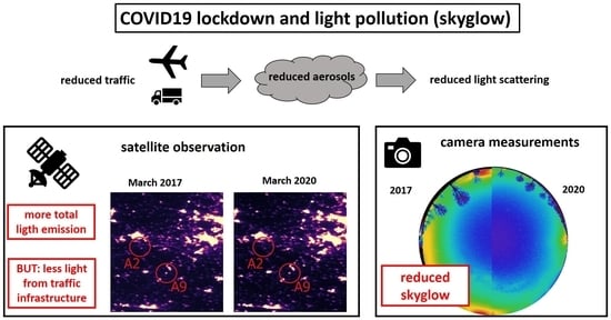
:Artificial skyglow, the brightening of the night sky by artificial light at night that is scattered back to Earth within the atmosphere, is detrimental to astronomical observations and has an impact on ecosystems as a form of light pollution. In this work, we investigated the impact of the lockdown caused by the COVID-19 pandemic on the urban skyglow of Berlin, Germany. We compared night sky brightness and correlated color temperature (CCT) measurements obtained with all-sky cameras during the COVID-19 lockdown in March 2020 with data from March 2017. Under normal conditions, we expected an increase in night sky brightness (or skyglow, respectively) and CCT because of the transition to LED. This is supported by a measured CCT shift to slightly higher values and a time series analysis of night-time light satellite data showing an increase in artificial light emission in Berlin. However, contrary to this observation, we measured a decrease in artificial skyglow at zenith by 20% at the city center and by more than 50% at 58 km distance from the center during the lockdown. We assume that the main cause for the reduction of artificial skyglow originates from improved air quality due to less air and road traffic, which is supported by statistical data and satellite image analysis. To our knowledge, this is the first reported impact of COVID-19 on artificial skyglow and we conclude that air pollution should shift more into the focus of light pollution research.
1. Introduction
The current pandemic caused by the novel severe acute respiratory syndrome corona virus (SARS-COV2) and the coronavirus disease that first occurred in Wuhan, China, in late 2019 (COVID-19) [1], has had a huge impact on modern societies [2,3,4,5,6,7,8,9,10,11] and changed human life dramatically in early 2020. Starting in Wuhan, China, in January 2020, several countries have imposed so-called “lockdowns” to parts or all of their territories. During these lockdowns, private and social life as well as industrial and commercial activities were reduced to a minimum to break the exponential increase in the infection chain of the pandemic and reduce the strain on health systems and reduce the fatality rate accordingly. Besides the effects on the growth rates of virus infections [2,3], these lockdowns had several unintended effects [4,5,6,7,8,9,10,11]. These include a negative impact on the economy [4], on mental health and sleeping behavior [5] or the food intake of obese children [6], but also unintended positive effects on the environment, including improved air quality in heavily industrialized areas [7], improved surface water quality [8,9] and the reduction of heavy metal pollution in subsurface waters [10].
Night-time lights or artificial light at night (ALAN) can be observed from space by satellite imagery [11,12,13] and can be used to track human activities, economic growth or decline, war crisis, natural disasters, etc. (see a recent review for night-time light technologies and applications in [12]). The excessive use of ALAN is a form of environmental pollution, light pollution, that is detrimental to night-time observations by astronomers [14]. However, ALAN can also have diverse negative impacts on flora and fauna in diverse habitats [15,16,17,18,19,20] and potentially human health [20,21].
Artificial skyglow is the brightening of the night sky that originates from ALAN that is scattered back towards Earth within the atmosphere [22,23]. This anthropogenic skyglow is very dynamic as it depends on atmospheric constituents like particulate matter from air pollution [24], weather-phenomena like clouds [25,26], ground reflectance [27] or the dynamics of ALAN sources itself [28,29,30,31]. Furthermore, there are other components like vehicle and residential lighting that contribute to skyglow but are difficult to disentangle from each other [31]. In a recent night-time satellite data analysis, an exponential growth rate in ALAN of more than 2% per year globally was determined [13]. A recent study of satellite night-time lights in China showed that the COVID-19 pandemic had a clear impact on night-time lights observed from space [11]. They found a decrease in night-time light emission in commercial areas, an increase in residential areas and a change in road illumination. However, to our knowledge, no study on the impact of COVID-19 on ALAN at ground level or on artificial skyglow exists to date.
In this paper, ground-based all-sky night-time photometry [32,33,34,35] was used to measure the night sky brightness, correlated color temperature (CCT) and illuminance at different distances from the city center of Berlin, Germany, during the COVID-19 lockdown in March 2020. Results are compared to measurements obtained in the same season and moon phase in March 2017 that were part of an investigation of the impact of clouds on the night sky brightness [35]. Furthermore, night-time light data from satellites and statistical data on air traffic were investigated to link it to the observations.
2. Materials and Methods
2.1. COVID-19 Lockdown in Germany, Spring 2020
Germany was the European country with the earliest detected COVID-19 patients with a small cluster with mild conditions [36]. The German government declared the Chinese province Wuhan as a risk region for travel on 26 January 2020, and in February 2020, several other countries were declared as risk regions as well [37]. A warning to avoid any travel to foreign countries was declared on 17 March 2020, and most borders were closed for travel. Social, cultural and commercial activities were slowly minimized in February starting with the ban of large-scale events. On 22 March 2020, the German government declared to reduce social life to an absolute minimum, to close bars restaurants, schools and alike and to keep distance. At this point, only essential businesses and industries were allowed to operate and most people were working from home, were on forced holiday or were on reduced work hours (“Kurzarbeit”), which was financially supported by the government. Air and road travel were reduced dramatically. This was the strongest part of the so called “lockdown” in Germany, which, however, was more relaxed than in other countries and did not include a strict curfew or similar measures.
2.2. Study Sites
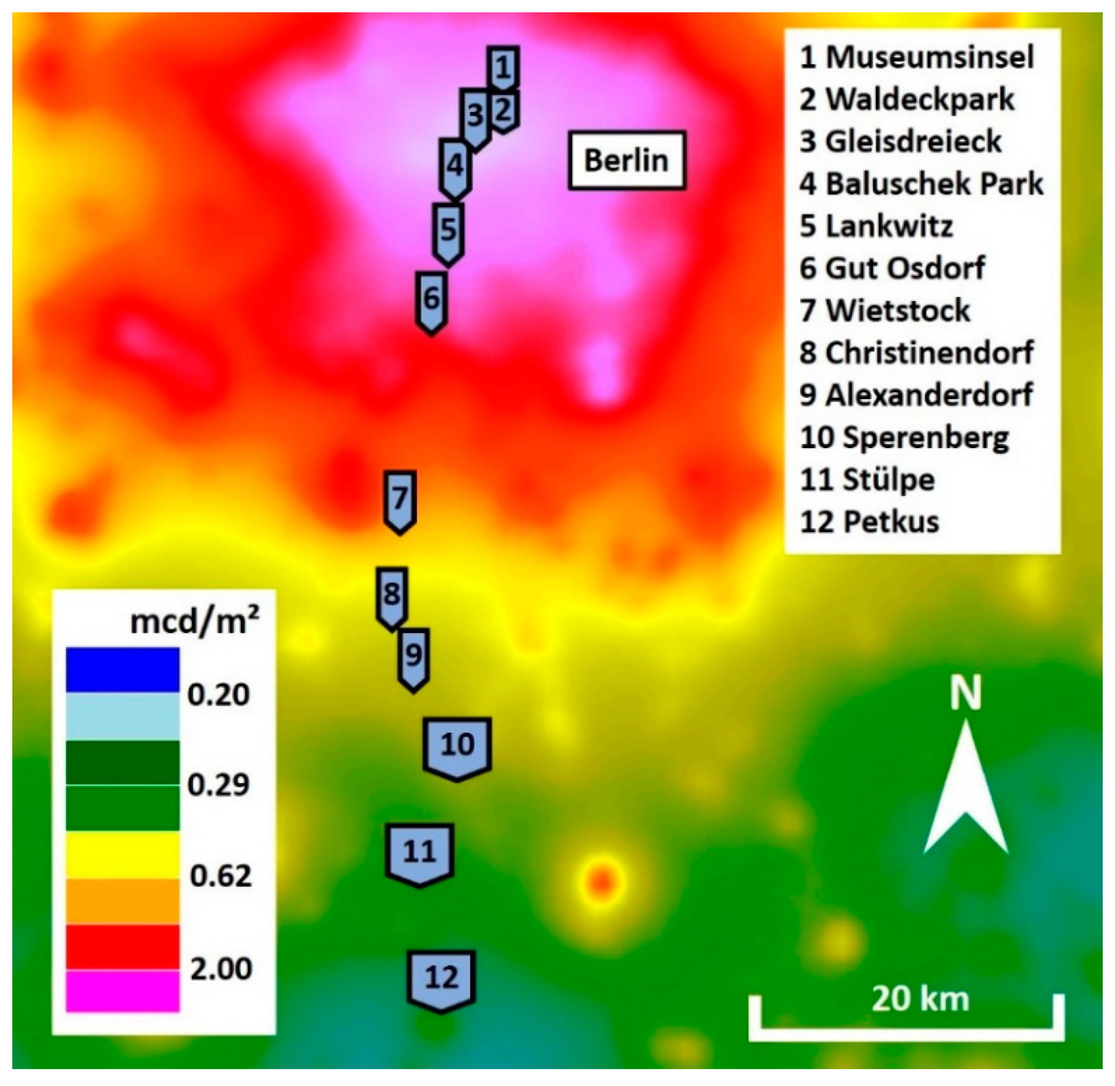
To determine the night-sky brightness at different distances from the city center of Berlin, a transect with twelve stops was designed during an earlier study that focused on the impact of clouds [35]. The stops ranged from the city center near Berlin, Alexanderplatz, to a rural location about 60 km south of the city center. A map of the stops is shown in Figure 1 using simulated skyglow data from Falchi et al. [23]. Five stops were within the city limit of Berlin and seven outside of the city limit. Sites were selected to have a minimum of direct lights incident at the camera. Thus, mostly urban parks were selected. The locations and measurement times are given in Table A1 in Appendix A and more details about site selection can be found in a recently published paper [35].
Measurements in 2017 were obtained during a clear night (0 octas) on 29 March during astronomical night between ca. 1:00 a.m. and 4:45 a.m. local time. The moon was at about 1% illumination, at a new moon and waxing crescent and between 27° and 35° below the horizon. Measurements in 2020 were performed on 26 March, which was a few days after the start of the strongest lockdown in Germany. Conditions were very similar to 2017 with a clear sky (0 octas). Measurements were obtained during astronomical night between 0:50 a.m. and 3:45 a.m. local time. The new moon was at about 0.5% illumination and between 29° and 40° below the horizon. These similar conditions should guarantee the smallest deviation possibly caused by seasonal or weather effects. Furthermore, the same seasonal period (late March) gives some confidences that hourly changes in human lighting behavior or automated switch-offs are very similar for the two nights studied. Furthermore, vegetation or ground albedo should be roughly similar (e.g., no snow on the ground).
2.3. Calibrated Camera System and Night Sky Brightness Processing Software
Ground-based all-sky night-time imagery was performed with a calibrated, commercial digital camera equipped with a fisheye lens [32,33,34,35]. The full procedure is described in detail in a recent method paper [34]. This method has several advantages compared to single channel photometers like the sky quality meters (SQMs) that are commonly used to monitor temporal changes of the night sky brightness but lack color and spatial information (see discussion in [34]). Briefly, a Canon EOS 6D with a Sigma EX DG circular fisheye lens with 180° field of view (f = 8 mm, aperture 3.5) was mounted on a tripod. Auxiliary equipment included a remote control, heating pads to avoid dew or ice formation on the lens, and a bull’s eye spirit level to align the camera with respect to the horizon.
To acquire all-sky images, most relevant for astronomical light pollution, the camera was aligned with the imaging sensor in the horizontal plane, i.e., the lens pointing towards the zenith. For pristine skies, the EOS 6D was operated at ISO 3200 or 6400, and up to 120 s exposure time. In urban environments, ISO 1600 and exposure times as short as a 0.4 s were used. The aperture was always set to a maximum of 3.5 and images were stored in an unaltered raw format.
The images were processed with a commercial software (“Sky Quality Camera” SQC version 1.8.1, Euromix, Ljubljana, Slovenia). SQC calculates luminance using the green channel of the camera and the photometric calibration is realized by star brightness and extinction measurements, while lens errors are corrected in the laboratory. The SQC software processes the luminance of the sky for each pixel of the camera. From the spatially resolved luminance maps, the software can derive the cosine corrected illuminance in the imaging plane (light that is falling in from zenith is weighted more than light incident at a shallow angle), and the scalar illuminance for the imaging hemisphere without cosine correction (light from all directions is weighted equally). From the three spectral channels, the correlated color temperature (CCT) can be calculated. For the definition and explanation of illuminances and the CCT calculation, see our method paper [34].
2.4. Night-Time Light Analysis
Monthly composites of night-time light data from the Suomi National Polar-Orbiting Partnership (NPP) instrument Visible Infrared Imaging Radiometer Suite (VIIRS) Day–Night Band (DNB) were used for the analysis, which are freely available at the website of the Earth Observation Group at Payne Institute [38]. These data were composed of moonless and cloud-free data and were shown to be a robust source for night-time light analysis [11,12,13]. The monthly compsites of March 2017 and March 2020 of the Tile2_75N060W (Europe) were downloaded and processed in QGIS (Version 3.10) [39]. The region of interest was plotted and the monthly composite data from March 2017 were subtracted from the March 2020 data.
The time series analysis was performed using the web tool radiance light trends [40] that allows the simple time-series analysis of small areas of VIIRS DNB data without any GIS skills. A polygon can be drawn or uploaded and then the time period and months of interest can be selected. The time frame between January 2017 and March 2020 was investigated for Berlin, the transect region investigated and several towns nearby and at the transect. The web app automatically selects the months between September and March for these latitudes to exclude twilight effects. More information on the location and the time series data for average radiance is given in the appendix.
3. Results
3.1. Ground-Gased Imaging Data
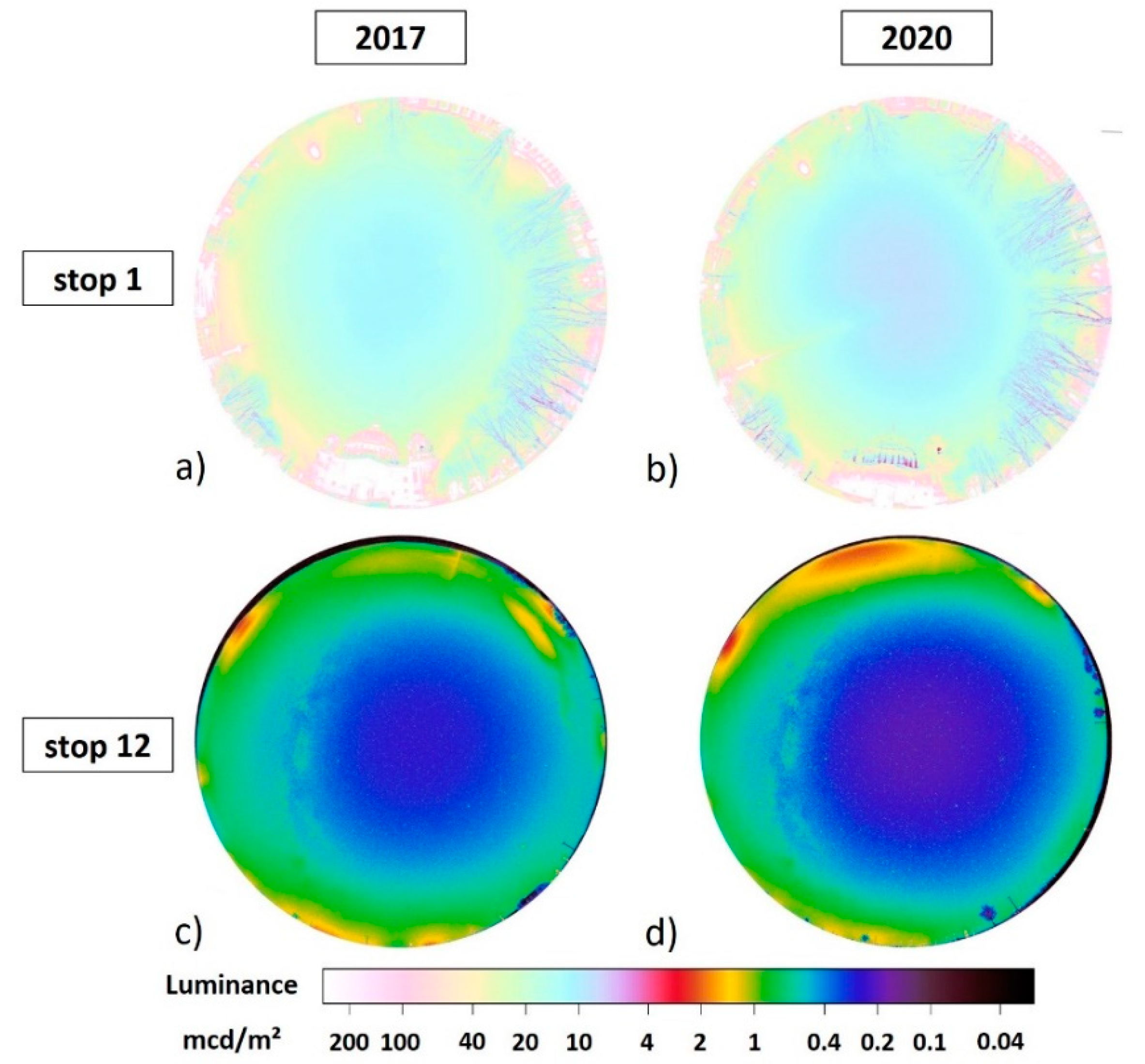
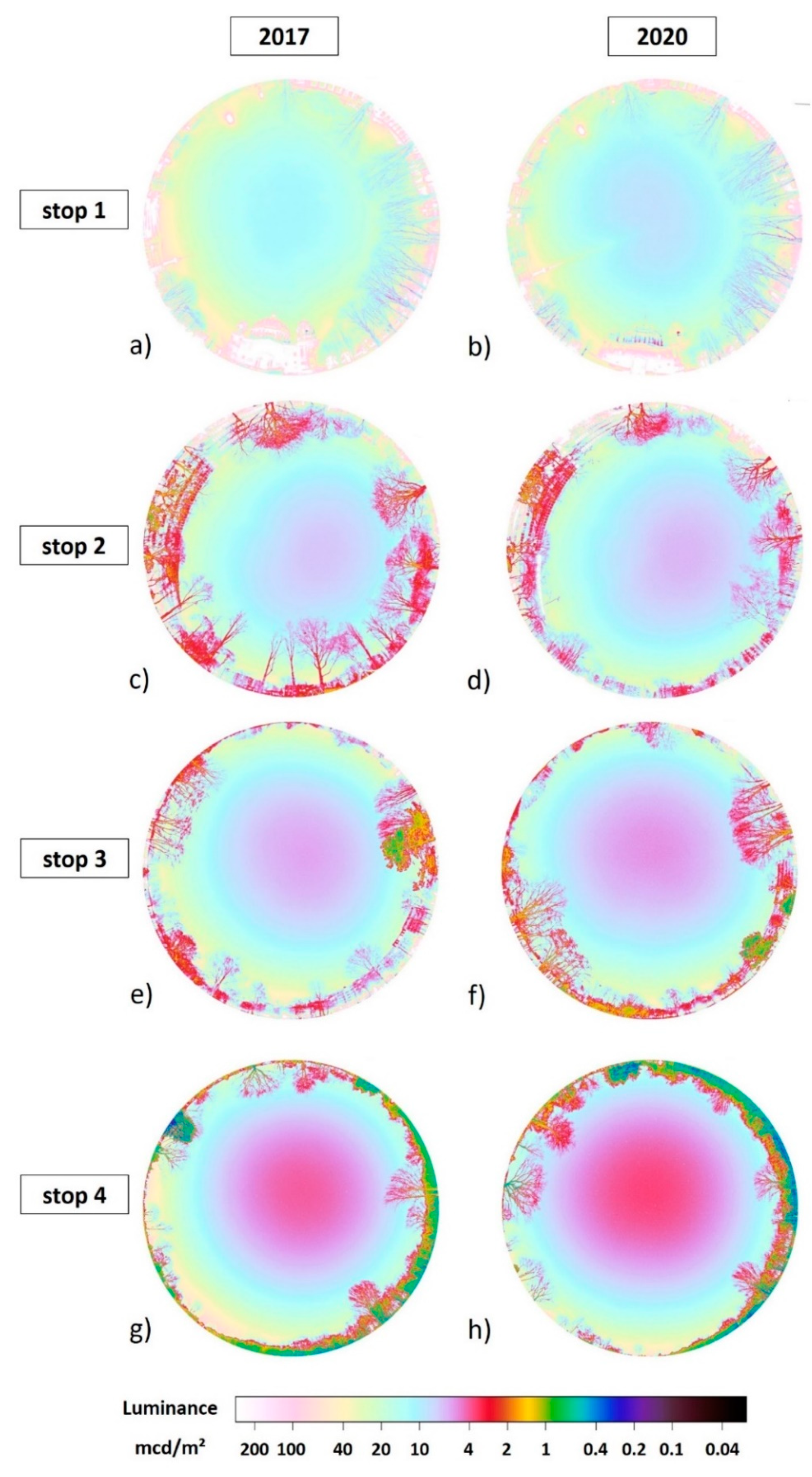
Figure 2 shows the luminance maps of two of the twelve stops for both measurement campaigns. The upper row shows the luminance data measured at stop 1, (Berlin Museumsinsel) just at the city center (0.3 km distance to Alexanderplatz) and the lower row the luminance data at stop 12 (Petkus) that are the farthest away from the city center (58.5 km). The left column shows data obtained in 2017 (no lockdown) and the right column the data obtained in 2020 (during lockdown). In the imaging data shown in Figure 2, a decrease in zenith brightness from the 2017 to the 2020 measurements can be assumed. There is a small shade in the center of Figure 2b and the dark blue region in Figure 2d is larger than in Figure 2c. Figure 3 shows the CCT maps of two of the twelve stops for both measurement campaigns in the same arrangement as in Figure 2. Here, the changes are even more obvious for the stop in the city center. For example, the light of the Berlin TV tower (lower left in Figure 3a,b) is switched on in 2020 (Figure 3b) but off in 2017 (Figure 3a).
3.2. Zenith Luminance and Artificial Skyglow
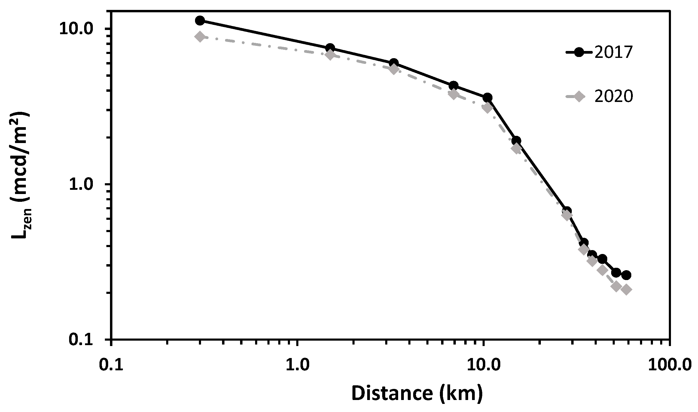
From the imaging data, the luminance at zenith , was extracted as defined by a 10 circle at the zenith (center of image). Figure 4 shows the zenith luminance for different distances for both datasets on a double logarithmic plot. It is obvious from the data, that the zenith brightness has decreased for all twelve measurement stops from 2017 to 2020. The full data are listed in Table 1 showing zenith luminance and radiance in units of the SQM. The strongest decrease in zenith brightness was observed at the city center. There, the luminance dropped from 11.30 mcd/m2 measured in 2017 to 8.90 mcd/m2 measured in 2020. Thus, the value obtained during the lockdown was 79% of the value measured earlier. At the two measurement points farthest away from the city center (stop 11 and 12), the zenith luminance measured during the lockdown was 81% of the value measured before. At stop 11, a luminance of 0.27 mcd/m2 (21.5 magSQM/arcs2) was measured in 2017 and a value of 0.22 mcd/m2 (21.7 magSQM/arcs2) was obtained in 2020. At stop 12, a luminance of 0.26 mcd/m2 (21.6 magSQM/arcs2) was obtained in 2017 and a value of 0.21 mcd/m2 (21.8 magSQM/arcs2) was measured in 2020. It is interesting to note that the luminance values obtained in 2020 in the rural locations are among the lowest zenith luminance values that we ever measured in the Berlin region for clear sky conditions.
The zenith luminance is the sum of the background sky luminance at zenith and the artificial skyglow component at zenith . Thus, the artificial skyglow component can be extracted (approximately) when subtracting the background from the actual measurement at the zenith:
A commonly used value for the sky background is 0.17 mcd/m2 (22.0 mag/arcs2) [23]. The corrected results are shown in Table 2. When considering the artificial zenith sky brightness only, the ratio between the values obtained in 2020 and 2017 decreased in the rural areas as expected. The biggest change occurred at the site farthest away from the center with more than a 50% decrease in artificial skyglow.
3.3. Illuminance
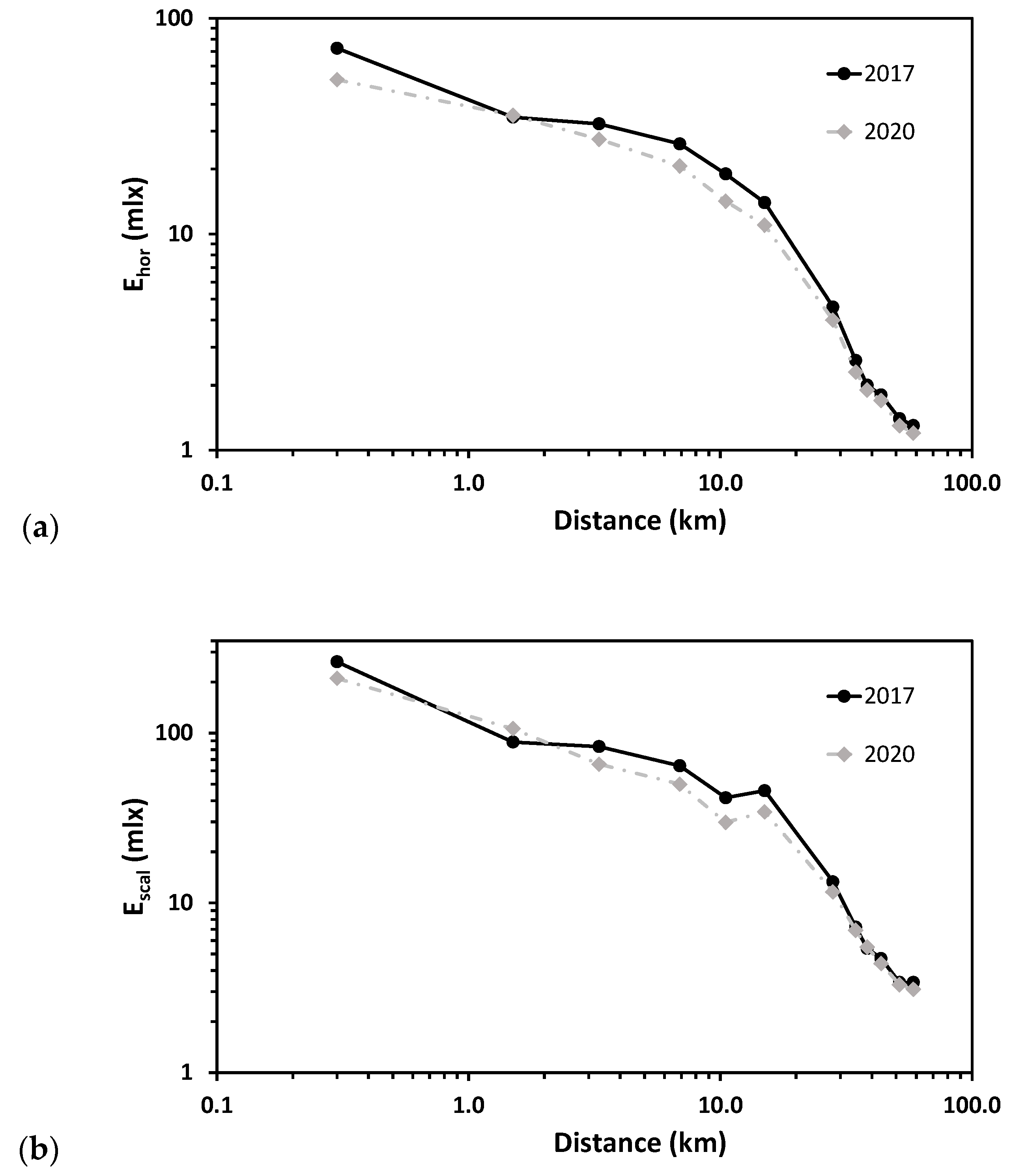
As outlined in the methods section, horizontal and (hemispheric) scalar illuminance can be calculated from the spatially resolved luminance maps. Figure 5 shows (a) the horizontal illuminance, and (b) the scalar illuminance for the different distances for both datasets on a double logarithmic plot. The data are listed in Table 3. For all measurement spots, apart from stop 2, the horizontal illuminance is reduced for the measurements obtained in 2020 compared to 2017. The strongest reduction was again observed in the city center at stop 1, where decreased from 72.6 mlx to 51.9 mlx to 71%. For , the reduction was less strong in the rural places than in the city center and the outskirts of the city. It is interesting, that for stop 2, was about the same for both measurements, although the zenith brightness had decreased by about 10% from 2017 to 2020. This was presumably caused by the lighting from the windows of buildings in the vicinity of the measurement stop.
For the (hemispheric) scalar illuminance, , the results were very similar to those for the horizontal illuminance. decreased most in the city center at stop 1 to 80% as well as just near the city border at stop 5 to 72% and just outside of the city at stop 6 to 75%. Just at stop 2 increased from 2017 to 2020 by about 20%, which again can be attributed to window lighting. At the rural locations farthest away from the city, decreased only by a few percent or remained about constant.
Please be aware that within the city limit, direct lights could not be fully avoided at all stops, although much care was taken (see methods section). However, outside of the city limit, the effect of nearby lamps on the illuminance can be largely ruled out.
3.4. Correlated Color Temperature
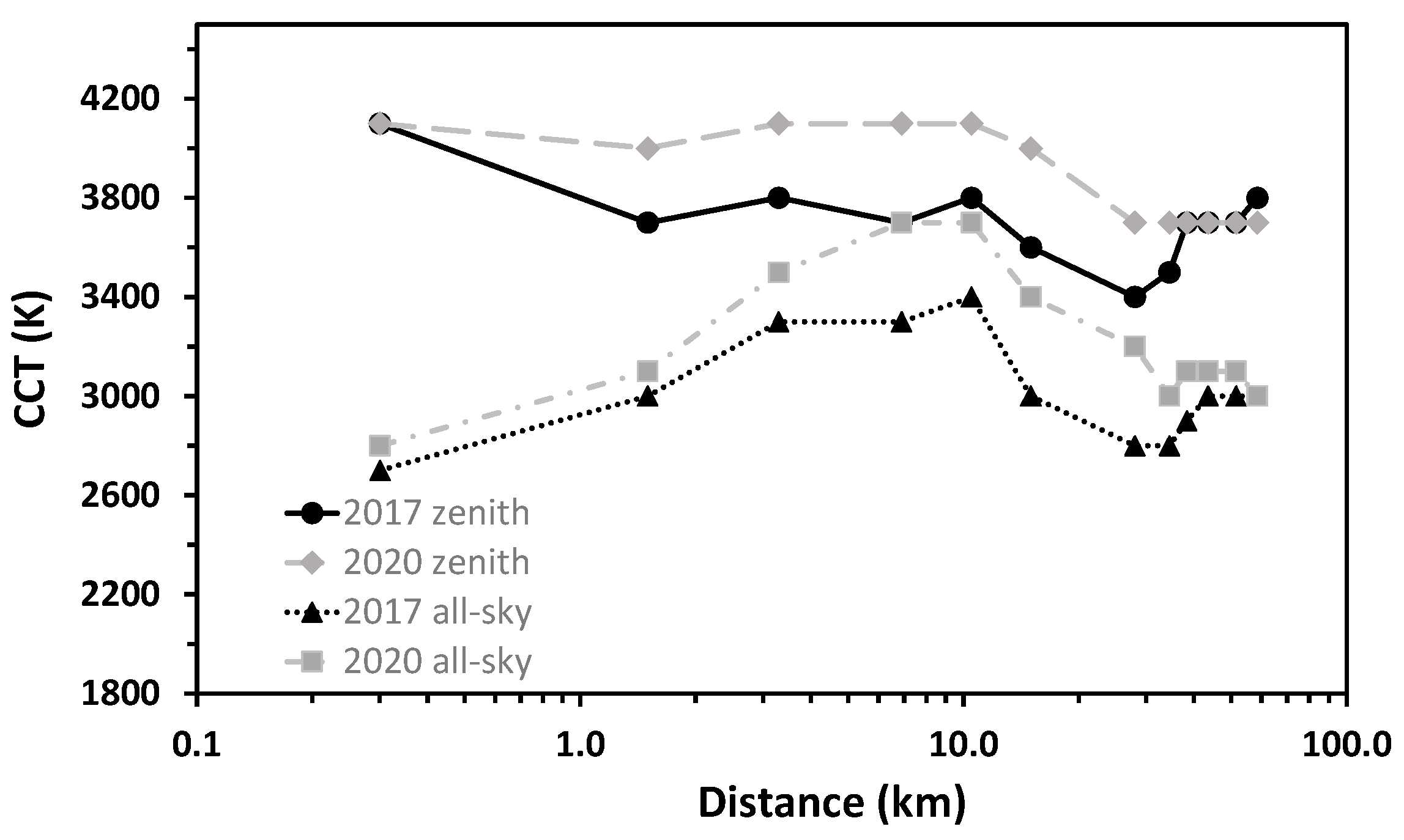
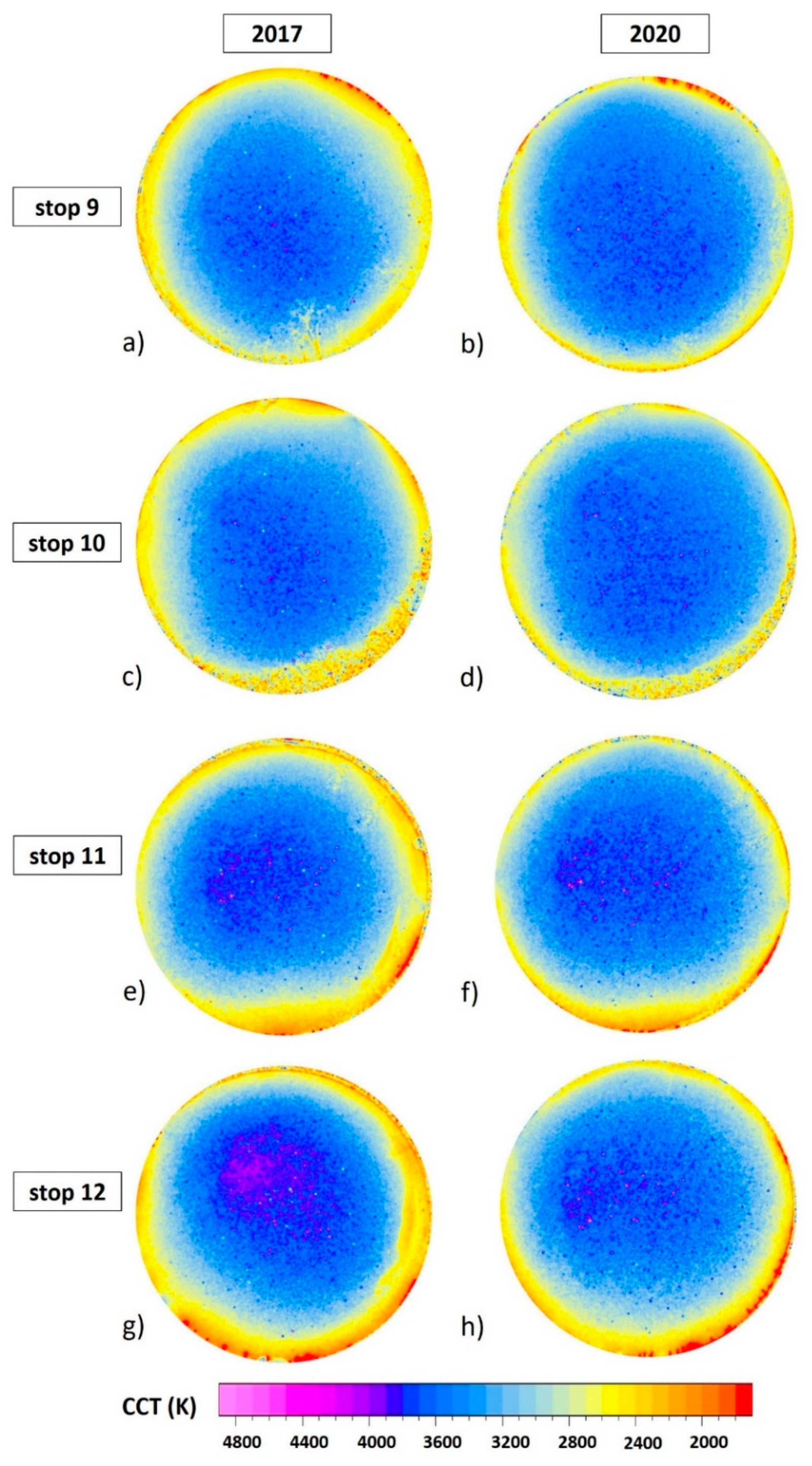
The CCT values for the full image and at the zenith were shown in Figure 6 for different distances to the city center. The CCT data are listen in Table 4. The CCT increased for 18 of the 24 data points, remained the same for five data points and decreased only at one data point. The highest increase was 300–400 K and occurred near the city edge or just outside of the city (stops 4–7), while in the city center and at large distances from the city the CCT remained rather constant. We noted that the TV tower lights seemed to have no measurable impact on the CCT at stop 1 although this was an obvious feature in the imaging data (see Figure 2a,b).
3.5. Night-Time Light Analysis
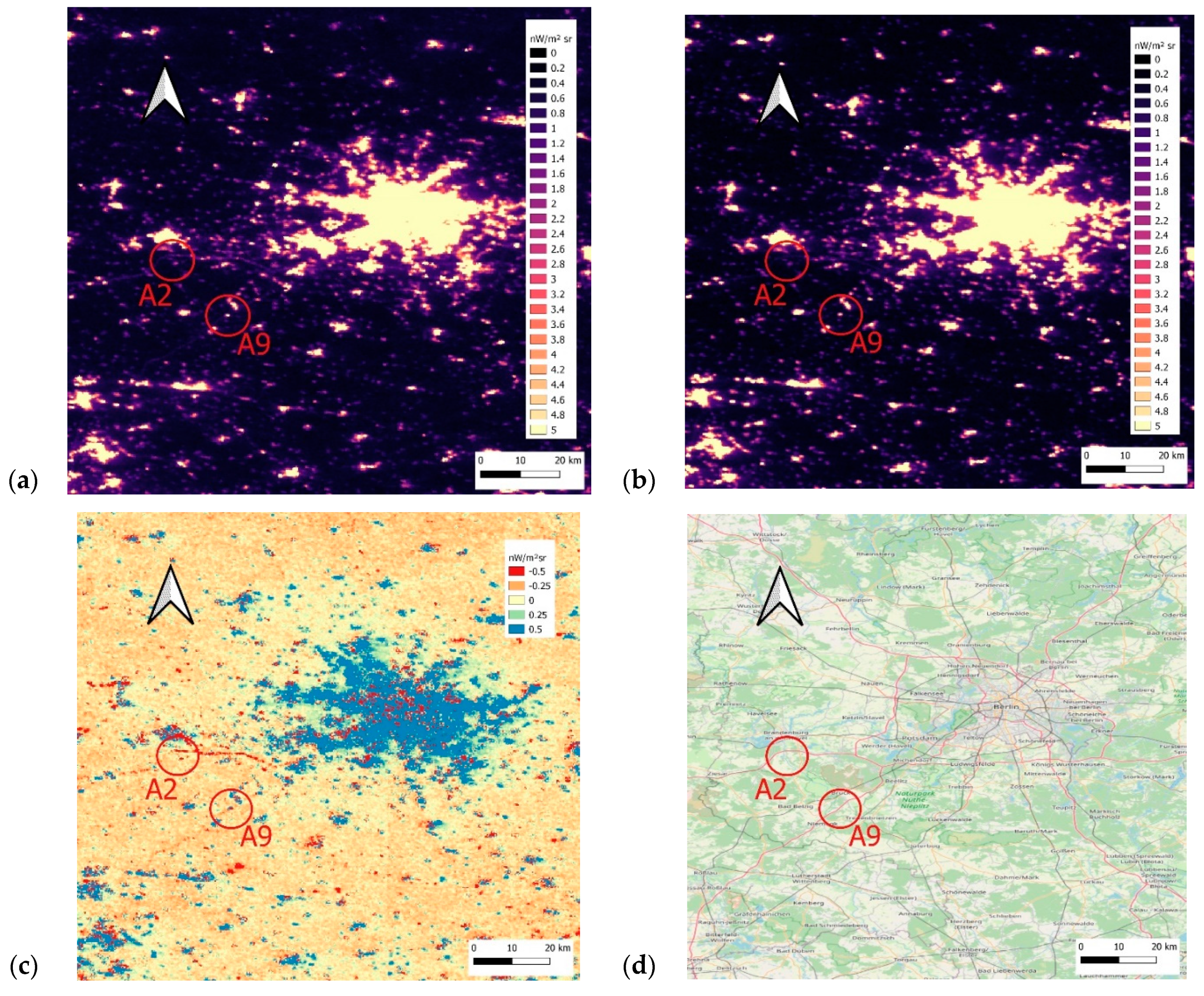
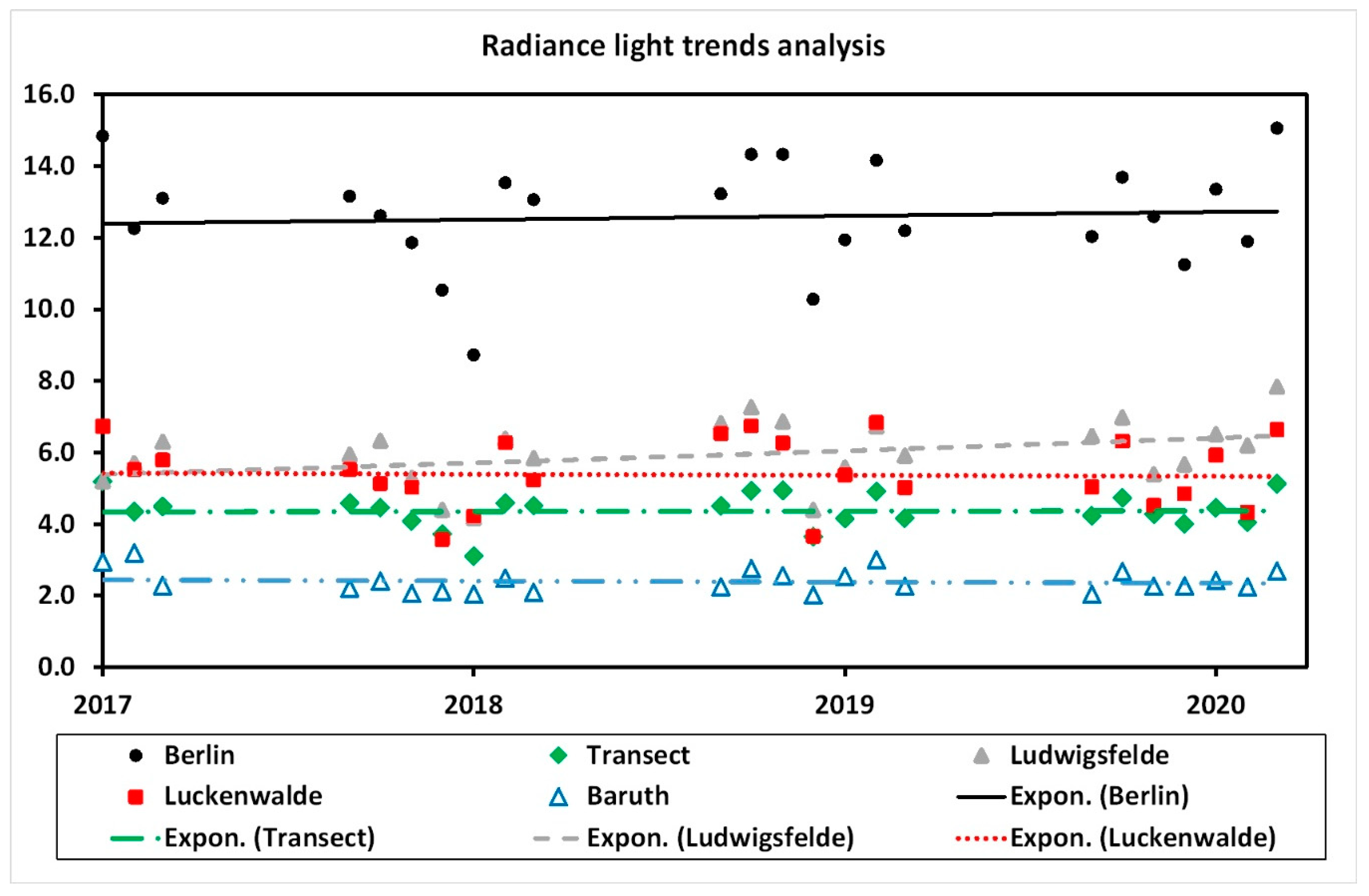
Figure 7 shows the VIIRS DNB monthly composites for (a) March 2017 and (b) March 2020. The subtraction of the March 2017 data from the March 2020 data is shown in Figure 7c and in a map in Figure 7d. Overall, the brightness in the area increased between March 2017 and March 2020 (see Figure 7c blue areas and also Appendix B for the time series analysis) particularly in the city center of Berlin and in the larger towns along the transect. A striking feature in the data is that the major motorways leading to the south and west of Berlin (A2 and A9 marked with red circles in Figure 7) are clearly visible in the 2017 data but not in the 2020 data. This is also visible in the subtracted data as red lines. The time series analysis (shown in Figure A7 in Appendix B) resulted in almost constant night-time light emission for the transect (−0.1%/y annual change), a small increase in Berlin (+0.6%/y), a small decrease for the town of Luckenwalde (−0.4%/y), a substantial increase in Ludwigsfelde, the largest town on the route outside of Berlin (+5.8%/y), and a decrease in Baruth, a smaller town near the route (−1.9%/y).
4. Discussion
The skyglow survey during the COVID-19 lockdown showed measurable differences in zenith luminance, illuminance, as well as changes in the CCT compared to earlier data. Since 2016, the state of Berlin has replaced conventional lighting technology, mainly high-pressure sodium lamps with LED luminaires and used LEDs for all new installations. Because high-pressure sodium lamps have a low CCT of typically 2100 K and the newly installed LEDs typically have a higher CCT between 3000 K and 4000 K, we expected that the CCT would have increased in Berlin. This is supported by our data as 18 of 24 measurement locations showed a higher CCT in 2020 compared to 2017.
Furthermore, an increase in the overall brightness was expected because typically highly efficient LED luminaires with higher luminous flux replaced older lamps. The number of LED luminaires is continuously growing in Berlin (19.500 LEDs in 2017 vs. 34,500 LEDs of 225,000 streetlights in December 2019) [41]. In contrast to this hypothesis, we observed a decrease in artificial skyglow (background corrected luminance at zenith) at all measurement points. In the center, the artificial skyglow component measured in 2020 decreased by more than 20% compared to that measured in 2017, although the TV tower was lit in 2020 and not in 2017. At the rural site farthest away from the city center, the artificial skyglow component decreased by more than 50% between 2017 and 2020. The illuminance decreased for almost all measurement stops apart from stop 2, which was the only one with buildings with windows nearby, that probably caused an increase of 20% for the scalar illuminance measurement. The highest decrease in illuminance was measured at the city center by almost 30%.
There are several potential causes for such a reduction in skyglow:
- Drastic natural atmospheric changes (desert dust, fires, volcanic ash);
- Seasonal changes (leaves, ground albedo, snow);
- Reduction of ALAN emissions by automated and manual switch offs;
- Change to modern (shielded) lighting technology [42];
- Anthropogenic atmospheric changes (air quality, air pollution);
- Reduction of ALAN emissions by changed behavior.
Several of these causes can be ruled out (or are at least unlikely). There were no reports of desert dust, fires or volcanic ash or any heavy snow event near both measurement periods. The measurements were (fortunately) timed during the same season, both during a working weekday (Wednesday in 2017 vs. Thursday in 2020), for very similar weather conditions (clear sky) and about the same moon illuminance (near new moon and well below horizon) and for almost exactly the same time. Thus, the external seasonal influences like ground albedo (snow, vegetation), shading by leaves, etc. should be minimized as much as possible. Furthermore, we expect that automated switch-offs of lighting that can occur late in the night are comparable between the observation period (weekday, same season).
Large-scale changes to modern and shielded lighting technology can be detected with all-sky imagery [42]. However, a change that explains the reduced artificial skyglow as strongly as we measured would have been detected as a large drop in night-time satellite data, particularly if this goes with a change to LED technology with a higher CCT. We indeed observed a slightly higher CCT with our ground-based measurements. Because the satellite sensor (VIIRS, DNB) lacks sensitivity for shortwave blue light that is stronger for modern LEDs, a change to LEDs at the same illuminance would appear as decrease for the satellite (see Figure 5 in [13]). However, our night-time light analysis shows no such drop in brightness but rather an increase in night-time light emission in Berlin and the largest town on the route. Thus, a strong increase in skyglow should be observed on the ground which is contrary to our observations.
This leaves anthropogenic atmospheric changes and changed light use behavior as the main causes of the observed reductions of skyglow. Atmospheric changes are highly likely because the travel in general and air traffic in particular were reduced dramatically. According to the statistics of the airports in Berlin [43], the air traffic in February 2020 was about the same as in February 2019 (−0.12%). However, in March 2020 the air traffic did decrease remarkably (−46.5%) compared to March 2019 and in April 2020 almost no air traffic was present compared to April 2019 (−93.2%). This was further supported by the data from the European Organization for the Safety of Air Navigation, EUROCONTROL, that show that for the 28 and 29 March 2020, the air traffic in Germany was reduced already by about 80% compared to the same day in 2019 [44].
The exhaust emission of aircrafts can produce contrails, which can be a source of very thin cirrus clouds that are difficult to detect but are assumed to play a complex role in climate change because of radiative forcing [45]. Modeled data for April 2020 using the EUROCONTROL data show a drastic reduction in contrails due to reduced air traffic during the COVID-19 pandemic [46]. Daytime aerosol optical depth (AOD) measurements show a slight decrease in the last hours before the nights of measurement from 2017 to 2020 (see Appendix C). The absence of polluting aerosols will reduce skyglow as shown in a study in Cracow, Poland [24], but also means less extinction towards the satellite, which is exactly what we have observed.
A side effect is that with reduced air and road traffic, also a part of the light that travels through the atmosphere horizontally (and that is most likely not detected by the satellites) will be reduced, which is one component of skyglow. How large the contribution of vehicle lighting to skyglow is remains an open research question. In a seminal work, Bará et al. used the temporal information of zenithal night sky brightness measured with an SQM in two towns in Galicia, Spain, to identify the contributions of different light sources [31]. By a modal expansion of the time representation they were able to acquire time signatures of the different sources of light. They concluded that the contribution of vehicles was rather small (few percent) in the larger town (A Coruña, 250,000 inhabitants), but larger (nearly 10%) in a smaller town (Arteixo, 30,000 inhabitants). No such data are available for Berlin and its surroundings. However, an aerial study in Berlin showed that lighting associated with streets has been found to be the dominant source of zenith directed light pollution (31.6%) [47]. We want to point out that this fraction largely depends on the amount of traffic and the number of lit roads, type of lamps and illumination levels. In a settlement with shielded lamps, few lit roads and low illumination levels but high traffic, this fraction could become substantial. The other component is changed lighting behavior during the pandemic like switching off public lighting such as road lights or private lights from large businesses etc. This is very difficult to disentangle as shown in a recent large-scale switch-off experiment [30]. Nevertheless, the night sky brightness decreased by about 20% in a switch-off for ornamental lights in a town in Catalunya, Spain [28], by more than 5% in the city center when switching off streetlights in Tucson, Arizona, USA [30], and by about 8% during the WWF Earth Hour 2018 in Berlin, Germany [29].
During the COVID-19 survey and later (personal observation, AJ) it seemed that no public lighting was reduced during the pandemic and that also most small business lights remained switched on. This could be explained by the fact that night-time lighting was not high up on the agenda of government decisions as there were so many urgent pandemic-related matters to be taken care of. Furthermore, night-time light seems to be also an inherent proxy of societal functionality as some newspapers were advertising “the lights will stay on during pandemic” [48].
5. Conclusions
In conclusion, it was possible to detect a reduction of skyglow during the COVID-19 lockdown in Berlin, Germany. This was surprising, because the overall light emission trend in the region as observed by satellite data was increasing. Luminance and illuminance decreased most strongly in the city center but also far away from the city. The strongest influence of the lockdown on the night sky brightness is assumed to originate from reduced air pollution due to a smaller reduction in industrial activity and dramatically reduced traffic. The latter is supported by statistical data of airport traffic and a comparison of the night-time satellite data where the road traffic reduced evidently. Other possible causes are changes in private lighting and reduced horizontal light from less traffic. Air pollution has not attracted much interest by the ALAN and the light pollution community to date. However, our results call for further interdisciplinary collaboration between health scientists, climate scientists, astronomers, and ecologists. A reduction of air pollution should also become a focus of light pollution research and mitigation efforts. A well managed use of sustainable and energy-efficient lighting technology will reduce energy consumption as well as unwanted ALAN emissions. In regions with electricity produced by fossil fuel, a reduction in energy consumption could also reduce air pollution.
Author Contributions
Conceptualization, A.J.; methodology, A.J.; validation, A.J.; formal analysis, A.J.; investigation, A.J. and F.H..; resources, A.J. and F.H.; data curation, A.J.; writing—original draft preparation, A.J.; writing—review and editing, F.H..; visualization, A.J. All authors have read and agreed to the published version of the manuscript.
Funding
This work received no external funding.
Acknowledgments
The authors thank Christopher C.M. Kyba who was involved in the design of the cloud study performed in 2017 of which part of the data was used. The publication of this article was funded by the Open Access Fund of the Leibniz Association and by the Open Access Fund of the Leibniz-Institute of Freshwater Ecology and Inland Fisheries (IGB).
Conflicts of Interest
The authors declare no conflict of interest.
Appendix A
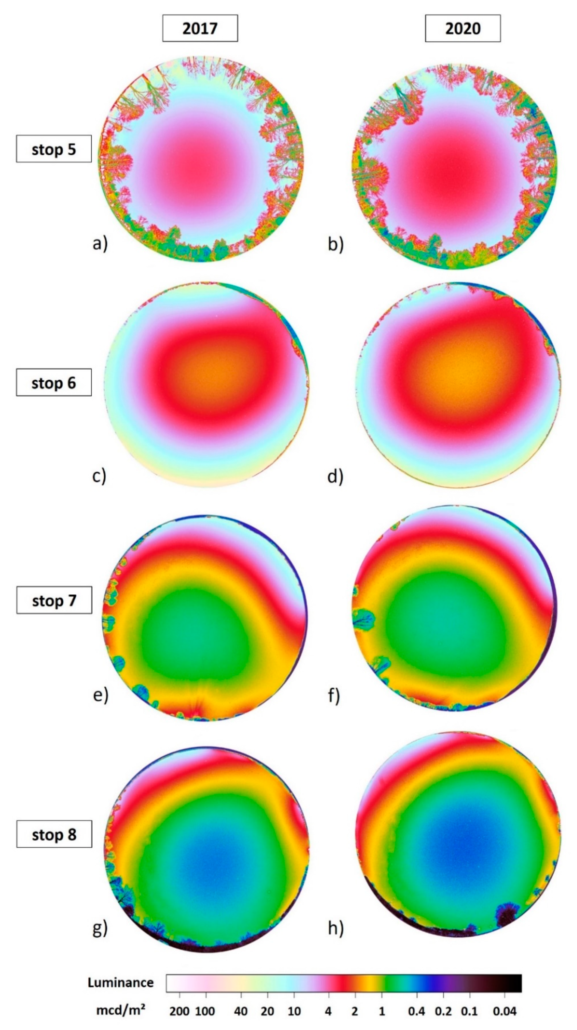
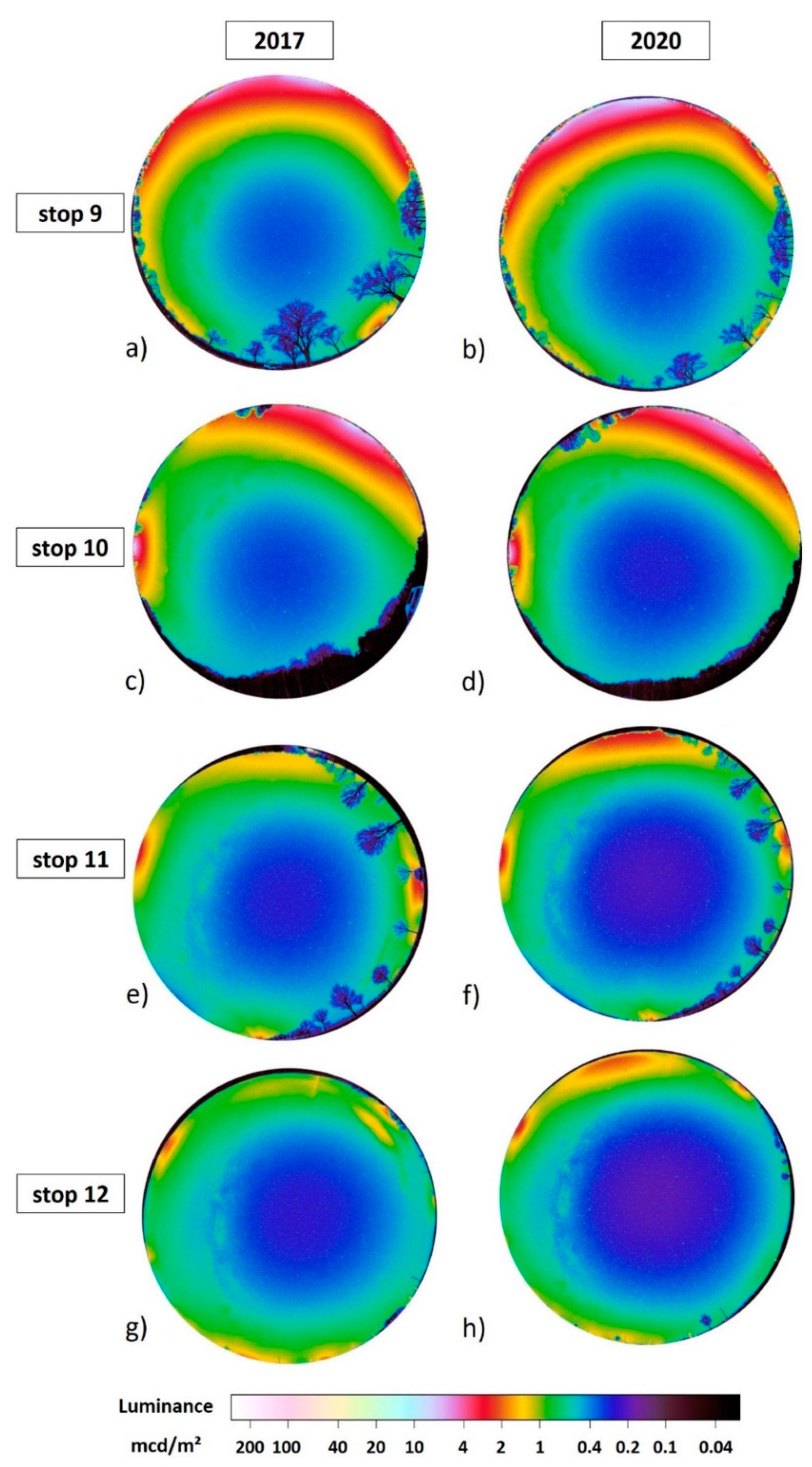
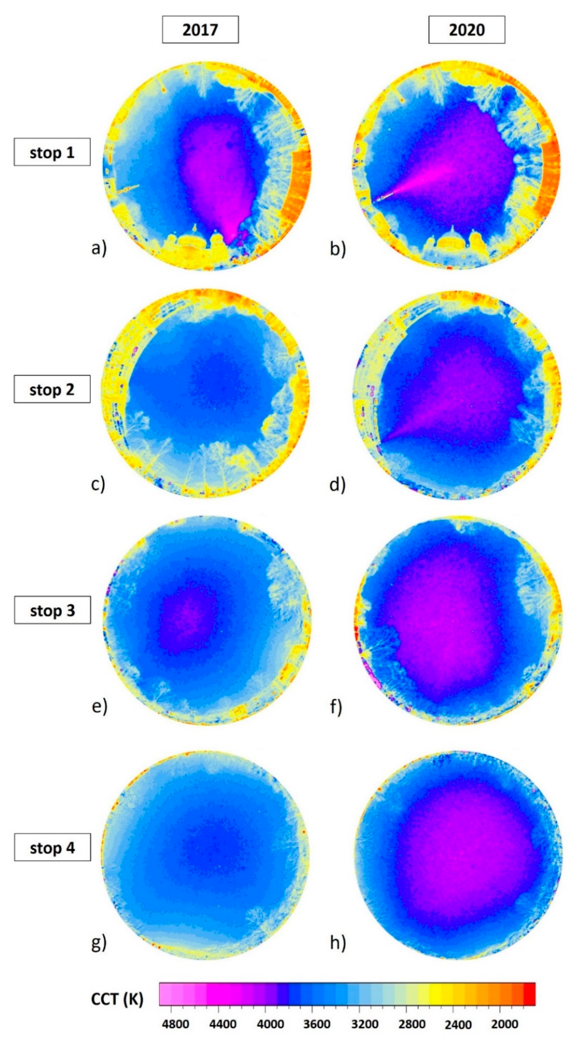
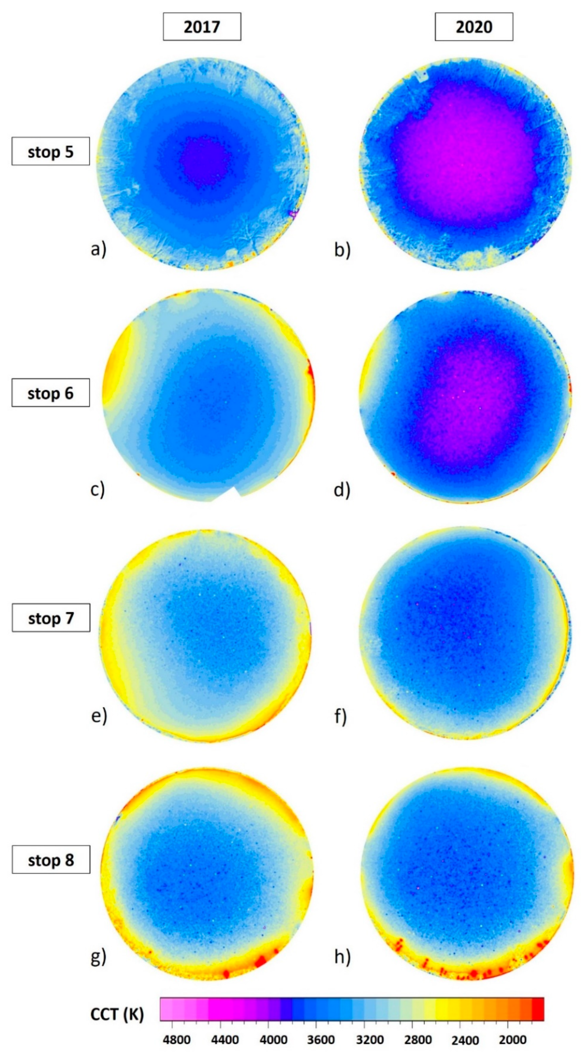
The full imaging dataset is shown here with Figure A1, Figure A2 and Figure A3 showing luminance maps and Figure A4, Figure A5 and Figure A6 showing CCT maps. The positions of the measurement locations and measurement times are given in Table A1.
Figure A1.
Luminance maps for stops 1–4. (a,c,e,g) 2017 data, (b,d,f,h) 2020 data.

Figure A2.
Luminance maps for stops 5–8. (a,c,e,g) 2017 data, (b,d,f,h) 2020 data.

Figure A3.
Luminance maps for stops 9–12. (a,c,e,g) 2017 data, (b,d,f,h) 2020 data.

Figure A4.
CCT maps for stops 1–4. (a,c,e,g) 2017 data, (b,d,f,h) 2020 data.

Figure A5.
CCT maps for stops 5–8. (a,c,e,g) 2017 data, (b,d,f,h) 2020 data.

Figure A6.
CCT maps for stops 9–12. (a,c,e,g) 2017 data, (b,d,f,h) 2020 data.


Table A1.
Information on the measurement locations, distance to city center and measurement times.
| Stop | Name | Distance (km) | Latitude | Longitude | 2017 Time | 2020 Time |
|---|---|---|---|---|---|---|
| 1 | Museumsinsel | 0.3 | 52.52004 | 13.39994 | 1:11 | 0:51 |
| 2 | Waldeckpark | 1.5 | 52.50654 | 13.40359 | 1:38 | 1:02 |
| 3 | Park am Gleisdreieck | 3.3 | 52.49472 | 13.3788 | 1:57 | 1:11 |
| 4 | Hans Baluschek Park | 6.9 | 52.46498 | 13.35863 | 2:23 | 1:27 |
| 5 | Gemeindepark Lankwitz | 10.5 | 52.43101 | 13.35208 | 2:44 | 1:45 |
| 6 | Gut Osdorf | 15 | 52.39304 | 13.33466 | 3:02 | 1:54 |
| 7 | Wietstock | 28 | 52.2761 | 13.30828 | 3:31 | 2:11 |
| 8 | Christinendorf | 34.5 | 52.21657 | 13.29815 | 3:56 | 2:30 |
| 9 | Alexanderdorf | 38.3 | 52.17978 | 13.31725 | 4:05 | 2:40 |
| 10 | Sperenberg | 43.5 | 52.12899 | 13.36726 | 4:19 | 2:55 |
| 11 | Stülpe | 51.5 | 52.06222 | 13.3261 | 4:31 | 3:09 |
| 12 | Petkus | 58.5 | 51.99443 | 13.35099 | 4:47 | 3:21 |
Appendix B
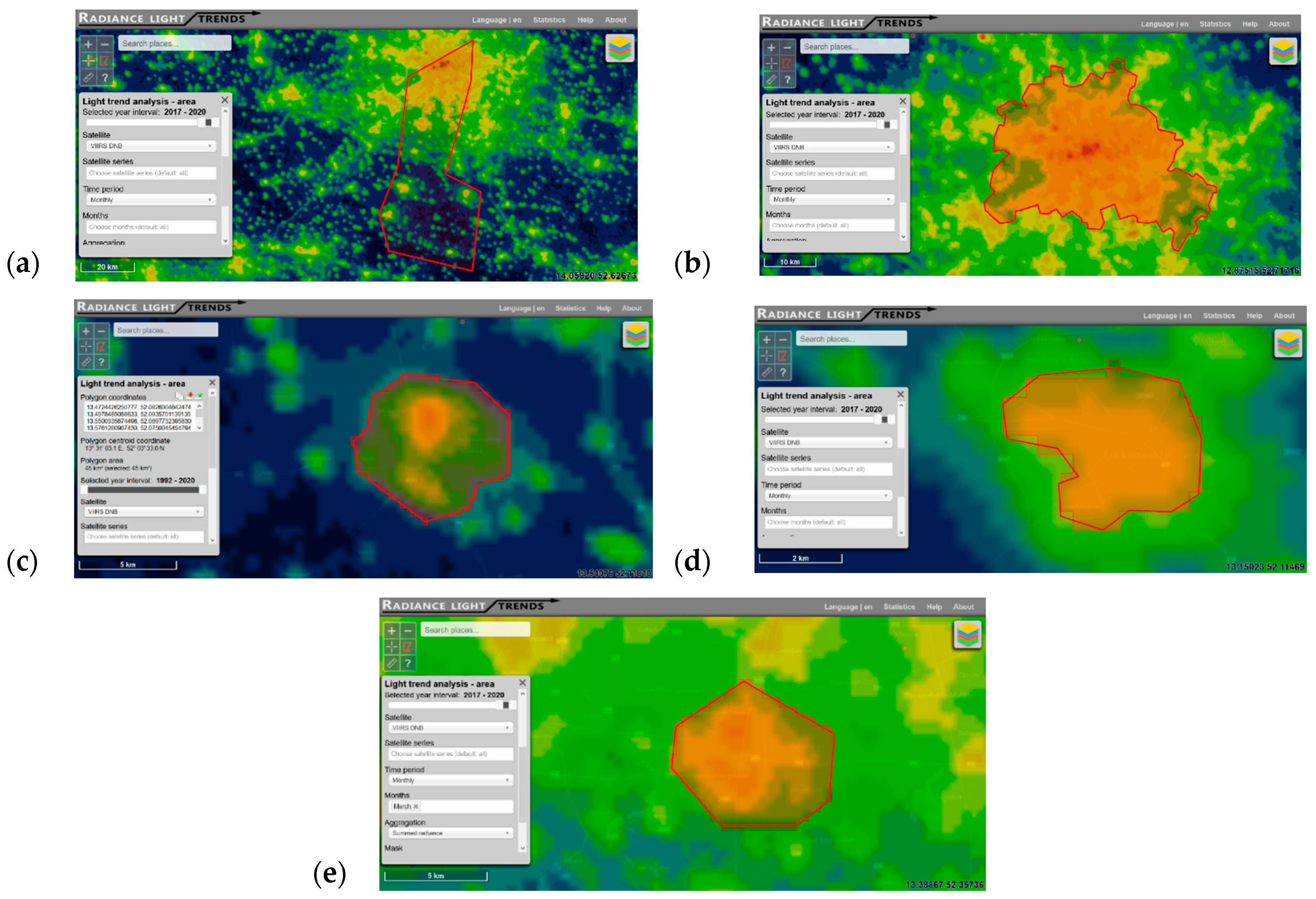
The VIIRS DNB time series data extracted from the web app “radiance light trends” [39] as well as the shapes of the selected polygons in the web app are shown in Figure A7 and Figure A8 for the transect (a), Berlin (b), the town of Baruth (c), the town of Luckenwalde (d) and the town of Ludwigsfelde (e). Furthermore, the light trends from the exponential fits through the monthly data are provided in Table A2.
Figure A7.
VIIRS DNB time series obtained from radiance light trend web tool [40] for the study area (green diamonds), Berlin (black solid circles), the town of Baruth (blue open triangles), the town of Luckenwalde (red solid squares) and the town of Ludwigsfelde (grey solid triangles). Exponential fits are shown in the same colors as the areas investigated.

Table A2.
Annual change in the average radiance for the areas investigated.
| Name | Annual Change |
|---|---|
| Transect area | −0.1%/y |
| Berlin | +0.6%/y |
| Ludwigsfelde | +5.8%/y |
| Luckenwalde | −0.4%/y |
| Baruth | −1.9%/y |
Figure A8.
VIIRS DNB time series obtained from radiance light trend web tool [39]: (a) the study area; (b) Berlin; (c) the town of Baruth; (d) the town of Luckenwalde; and (e) the town of Ludwigsfelde.
Figure A8.
VIIRS DNB time series obtained from radiance light trend web tool [39]: (a) the study area; (b) Berlin; (c) the town of Baruth; (d) the town of Luckenwalde; and (e) the town of Ludwigsfelde.

Appendix C
Aerosol optical depth was retrieved from the AERONET measurement station at Freie Universität Berlin (FUB). Only data for the days before the measurements were available for both years. The data of the last two hours of the day were averaged for the values given for 675 nm, 500 nm and 440 nm. The result is listed in Table A3.
Table A3.
Aerosol optical depth (AOD) for the three wavelengths in the visible range obtained from the AERONET measurement station at Freie Universität Berlin.
Table A3.
Aerosol optical depth (AOD) for the three wavelengths in the visible range obtained from the AERONET measurement station at Freie Universität Berlin.
| AERONET FUB | 28 March 2017 | 25 March 2020 |
|---|---|---|
| AOD 440 nm | 0.19 | 0.18 |
| AOD 500 nm | 0.17 | 0.15 |
| AOD 675 nm | 0.13 | 0.1 |
References
- Gorbalenya, A.E.; Baker, S.C.; Baric, R.S.; de Groot, R.J.; Drosten, C.; Gulyaeva, A.A.; Haagmans, B.L.; Lauber, C.; Leontovich, A.M.; Neuman, B.W.; et al. The species Severe acute respiratory syndrome-related coronavirus: Classifying 2019-nCoV and naming it SARS-CoV-2. Nat. Microbiol. 2020, 5, 536. [Google Scholar]
- Lau, H.; Khosrawipour, V.; Kocbach, P.; Mikolajczyk, A.; Schubert, J.; Bania, J.; Khosrawipour, T. The positive impact of lockdown in Wuhan on containing the COVID-19 outbreak in China. J. Travel Med. 2020, 27, taaa037. [Google Scholar] [CrossRef] [PubMed] [Green Version]
- Shen, M.; Peng, Z.; Guo, Y.; Xiao, Y.; Zhang, L. Lockdown may partially halt the spread of 2019 novel coronavirus in Hubei province, China. medRxiv 2020. [Google Scholar] [CrossRef] [Green Version]
- Moser, C.A.; Yared, P. Pandemic Lockdown: The Role of Government Commitment; No. w27062; National Bureau of Economic Research: Cambridge, MA, USA, 2020. [Google Scholar]
- Gualano, M.R.; Lo Moro, G.; Voglino, G.; Bert, F.; Siliquini, R. Effects of COVID-19 lockdown on mental health and sleep disturbances in Italy. Int. J. Environ. Res. Public Health 2020, 17, 4779. [Google Scholar] [CrossRef] [PubMed]
- Pietrobelli, A.; Pecoraro, L.; Ferruzzi, A.; Heo, M.; Faith, M.; Zoller, T.; Antoniazzi, F.; Piacentini, G.; Fearnbach, S.N.; Heymsfield, S.B. Effects of COVID-19 lockdown on lifestyle behaviors in children with obesity living in Verona, Italy: A longitudinal study. Obesity 2020, 28, 1382–1385. [Google Scholar] [CrossRef] [PubMed]
- Mahato, S.; Pal, S.; Ghosh, K.G. Effect of lockdown amid COVID-19 pandemic on air quality of the megacity Delhi, India. Sci. Total Environ. 2020, 730, 139086. [Google Scholar] [CrossRef]
- Yunus, A.P.; Masago, Y.; Hijioka, Y. COVID-19 and surface water quality: Improved lake water quality during the lockdown. Sci. Total Environ. 2020, 731, 139012. [Google Scholar] [CrossRef]
- Niroumand-Jadidi, M.; Bovolo, F.; Bruzzone, L.; Gege, P. Physics-based bathymetry and water quality retrieval using planetscope imagery: Impacts of 2020 Covid-19 lockdown and 2019 extreme flood in the Venice Lagoon. Remote Sens. 2020, 12, 2381. [Google Scholar] [CrossRef]
- Selvam, S.; Jesuraja, K.; Venkatramanan, S.; Chung, S.Y.; Roy, P.D.; Muthukumar, P.; Kumar, M. Imprints of pandemic lockdown on subsurface water quality in the coastal industrial city of Tuticorin, south India: A revival perspective. Sci. Total Environ. 2020, 738, 139848. [Google Scholar] [CrossRef]
- Liu, Q.; Sha, D.; Liu, W.; Houser, P.; Zhang, L.; Hou, R.; Lan, H.; Flynn, C.; Lu, M.; Hu, T.; et al. Spatiotemporal patterns of Covid-19 impact on human activities and environment in mainland china using nighttime light and air quality data. Remote Sens. 2020, 12, 1576. [Google Scholar] [CrossRef]
- Levin, N.; Kyba, C.C.; Zhang, Q.; de Miguel, A.S.; Román, M.O.; Li, X.; Portnov, B.A.; Molthan, A.L.; Jechow, A.; Miller, S.D.; et al. Remote sensing of night lights: A review and an outlook for the future. Remote Sens. Environ. 2020, 237, 111443. [Google Scholar] [CrossRef]
- Kyba, C.C.M.; Kuester, T.; Sanchez de Miguel, A.; Baugh, K.; Jechow, A.; Hölker, F.; Bennie, J.; Elvidge, C.D.; Gaston, K.J.; Guanter, L. Artificially lit surface of Earth at night increasing in radiance and extent. Sci. Adv. 2017, 3, e1701528. [Google Scholar] [CrossRef] [Green Version]
- Riegel, K.W. Light pollution. Science 1973, 179, 1285–1291. [Google Scholar] [CrossRef]
- Schroer, S.; Hölker, F. Impact of lighting on flora and fauna. In Handbook of Advanced Lighting Technology; Karlicek, R., Sun, C.C., Zissis, G., Ma, R., Eds.; Springer: Cham, Switzerland, 2017; pp. 957–989. [Google Scholar]
- Longcore, T.; Rich, C. Ecological light pollution. Front. Ecol. Environ. 2004, 2, 191–198. [Google Scholar] [CrossRef]
- Matzke, E.B. The effect of street lights in delaying leaf-fall in certain trees. Am. J. Bot. 1936, 23, 446–452. [Google Scholar] [CrossRef]
- Robert, K.A.; Lesku, J.A.; Partecke, J.; Chambers, B. Artificial light at night desynchronizes strictly seasonal reproduction in a wild mammal. Proc. R. Soc. Lond. B Biol. Sci. 2015, 282, 20151745. [Google Scholar] [CrossRef] [Green Version]
- Kurvers, R.H.J.M.; Drägestein, J.; Hölker, F.; Jechow, A.; Krause, J.; Bierbach, D. Artificial light at night affects emergence from a refuge and space use in guppies. Sci. Rep. 2018, 8, 14131. [Google Scholar] [CrossRef] [Green Version]
- Grubisic, M.; Haim, A.; Bhusal, P.; Dominoni, D.M.; Gabriel, K.; Jechow, A.; Kupprat, F.; Lerner, A.; Marchant, P.; Riley, W.; et al. Light pollution, circadian photoreception, and melatonin in vertebrates. Sustainability 2019, 11, 6400. [Google Scholar] [CrossRef] [Green Version]
- Cho, Y.; Ryu, S.H.; Lee, B.R.; Kim, K.H.; Lee, E.; Choi, J. Effects of artificial light at night on human health: A literature review of observational and experimental studies applied to exposure assessment. Chronobiol. Int. 2015, 32, 1294–1310. [Google Scholar] [CrossRef]
- Aubé, M. Physical behaviour of anthropogenic light propagation into the nocturnal environment. Philos. Trans. R. Soc. B Biol. Sci. 2015, 370, 20140117. [Google Scholar] [CrossRef] [Green Version]
- Falchi, F.; Cinzano, P.; Duriscoe, D.; Kyba, C.C.M.; Elvidge, C.D.; Baugh, K.; Portnov, B.A.; Rybnikova, N.A.; Furgoni, R. The new world atlas of artificial night sky brightness. Sci. Adv. 2016, 2, e1600377. [Google Scholar] [CrossRef] [PubMed] [Green Version]
- Ściężor, T.; Kubala, M. Particulate matter as an amplifier for astronomical light pollution. Mon. Not. R. Astron. Soc. 2014, 444, 2487–2493. [Google Scholar] [CrossRef] [Green Version]
- Jechow, A.; Kolláth, Z.; Ribas, S.J.; Spoelstra, H.; Hölker, F.; Kyba, C.C.M. Imaging and mapping the impact of clouds on skyglow with all-sky photometry. Sci. Rep. 2017, 7, 6741. [Google Scholar] [CrossRef] [PubMed]
- Jechow, A.; Hölker, F.; Kyba, C. Using all-sky differential photometry to investigate how nocturnal clouds darken the night sky in rural areas. Sci. Rep. 2019, 9, 1391. [Google Scholar] [CrossRef] [PubMed] [Green Version]
- Jechow, A.; Hölker, F. Snowglow—The amplification of skyglow by snow and clouds can exceed full moon illuminance in suburban areas. J. Imaging 2019, 5, 69. [Google Scholar] [CrossRef] [Green Version]
- Jechow, A.; Ribas, S.J.; Domingo, R.C.; Hölker, F.; Kolláth, Z.; Kyba, C.C.M. Tracking the dynamics of skyglow with differential photometry using a digital camera with fisheye lens. J. Quant. Spectrosc. Radiat. Transf. 2018, 209, 212–223. [Google Scholar] [CrossRef] [Green Version]
- Jechow, A. Observing the impact of WWF Earth hour on urban light pollution: A case study in Berlin 2018 using differential photometry. Sustainability 2019, 11, 750. [Google Scholar] [CrossRef] [Green Version]
- Barentine, J.C.; Kundracik, F.; Kocifaj, M.; Sanders, J.C.; Esquerdo, G.A.; Dalton, A.M.; Foott, B.; Grauer, A.; Tucker, S.; Kyba, C.C. Recovering the city street lighting fraction from skyglow measurements in a large-scale municipal dimming experiment. J. Quant. Spectrosc. Radiat. Transf. 2020, 253, 107120. [Google Scholar] [CrossRef]
- Bará, S.; Rodríguez-Arós, Á.; Pérez, M.; Tosar, B.; Lima, R.C.; Sánchez de Miguel, A.; Zamorano, J. Estimating the relative contribution of streetlights, vehicles, and residential lighting to the urban night sky brightness. Lighting Res. Technol. 2019, 51, 1092–1107. [Google Scholar] [CrossRef] [Green Version]
- Kolláth, Z.; Dömény, A. Night sky quality monitoring in existing and planned dark sky parks by digital cameras. Int. J. Sustain. Light. 2017, 19, 61–68. [Google Scholar] [CrossRef]
- Kolláth, Z. Measuring and modelling light pollution at the Zselic Starry Sky Park. In Journal of Physics: Conference Series; IOP Publishing: Bristol, UK, 2010; Volume 218, p. 012001. [Google Scholar]
- Jechow, A.; Kyba, C.C.; Hölker, F. Beyond all-sky: Assessing ecological light pollution using multi-spectral full-sphere fisheye lens imaging. J. Imaging 2019, 5, 46. [Google Scholar] [CrossRef] [Green Version]
- Jechow, A.; Kyba, C.C.; Hölker, F. Mapping the brightness and color of urban to rural skyglow with all-sky photometry. J. Quant. Spectrosc. Radiat. Transf. 2020, 250, 106988. [Google Scholar] [CrossRef]
- Dieter, H. Germany in the COVID-19 crisis: Poster child or just lucky? J. Aust. Political Econ. 2020, 85, 101. [Google Scholar]
- Buecker, S.; Horstmann, K.T.; Krasko, J.; Kritzler, S.; Terwiel, S.; Kaiser, T.; Luhmann, M. Changes in daily loneliness during the first four weeks of the Covid-19 lockdown in Germany. PsyArXiv 2020. [Google Scholar] [CrossRef]
- VIIRS Day Night Band (DNB) Night-Time Lights Monthly Composites. Available online: https://eogdata.mines.edu/download_dnb_composites.html (accessed on 25 September 2020).
- QGIS Geographic Information System. Open Source Geospatial Foundation Project. Available online: http://qgis.org (accessed on 11 November 2019).
- Stare, J.; Kyba, C. Radiance Light Trends [web application]. GFZ Data Serv. 2019. [Google Scholar] [CrossRef]
- Berlin.de. Umwelt, Verkehr und Klimaschutz “Elektrische Beleuchtung”. Available online: https://www.berlin.de/sen/uvk/verkehr/infrastruktur/oeffentliche-beleuchtung/elektrische-beleuchtung/ (accessed on 26 September 2020).
- Kolláth, Z.; Dömény, A.; Kolláth, K.; Nagy, B. Qualifying lighting remodelling in a Hungarian city based on light pollution effects. J. Quant. Spectrosc. Radiat. Transf. 2016, 181, 46–51. [Google Scholar] [CrossRef]
- Airport Berlin Brandenburg Flight Statistics. Available online: https://www.berlin-airport.de/en/press/background-information/traffic-statistics/index.php (accessed on 26 September 2020).
- EUROCONTROL COVID-19 Daily Airtraffic Variation Dashboard. Available online: https://www.eurocontrol.int/Economics/DailyTrafficVariation-States.html (accessed on 29 September 2020).
- Burkhardt, U.; Kärcher, B. Global radiative forcing from contrail cirrus. Nat. Clim. Chang. 2011, 1, 54–58. [Google Scholar] [CrossRef] [Green Version]
- DLR Press Release “Up to 90 Percent Fewer Condensation Trails Due to Reduced Air Traffic over Europe”. Available online: https://www.dlr.de/content/en/articles/news/2020/02/20200520_fewer-condensation-trails-due-to-reduced-air-traffic.html (accessed on 29 September 2020).
- Kuechly, H.U.; Kyba, C.C.; Ruhtz, T.; Lindemann, C.; Wolter, C.; Fischer, J.; Hölker, F. Aerial survey and spatial analysis of sources of light pollution in Berlin, Germany. Remote Sens. Environ. 2012, 126, 39–50. [Google Scholar] [CrossRef]
- LA Times. How Power Companies are Keeping Your Lights on during the Pandemic. Available online: https://www.latimes.com/environment/story/2020-03-19/how-power-companies-are-keeping-your-lights-on-during-the-pandemic (accessed on 26 September 2020).
Figure 1.
Map of the transect stops around the city of Berlin, Germany using modeled skyglow data from the world atlas of artificial night sky brightness [23] for the Berlin area (source: lightpollutionmap.info by Jurij Stare).
Figure 1.
Map of the transect stops around the city of Berlin, Germany using modeled skyglow data from the world atlas of artificial night sky brightness [23] for the Berlin area (source: lightpollutionmap.info by Jurij Stare).

Figure 2.
Luminance maps for two of the twelve stops near Berlin Germany. (a,b) stop 1 near city center and (c,d) stop 12 farthest away from the city center. (a,c) 2017—no lockdown and (b,d) 2020—lockdown. The full imaging dataset is given in Appendix A.
Figure 2.
Luminance maps for two of the twelve stops near Berlin Germany. (a,b) stop 1 near city center and (c,d) stop 12 farthest away from the city center. (a,c) 2017—no lockdown and (b,d) 2020—lockdown. The full imaging dataset is given in Appendix A.

Figure 3.
Correlated color temperature (CCT) maps for two of the twelve stops near Berlin, Germany. (a,b) stop 1 near city center, and (c,d) stop 12 farthest away from the city center. (a,c) 2017—no lockdown and (b), and (d) 2020—lockdown. The full imaging dataset is given in Appendix A.
Figure 3.
Correlated color temperature (CCT) maps for two of the twelve stops near Berlin, Germany. (a,b) stop 1 near city center, and (c,d) stop 12 farthest away from the city center. (a,c) 2017—no lockdown and (b), and (d) 2020—lockdown. The full imaging dataset is given in Appendix A.

Figure 4.
Zenith luminance at different distances from the city center of Berlin, Germany, measured during a clear night in 2017 (black solid line and circles) and a clear night during the COVID-19 lockdown in 2020 (grey dashed dotted line and boxes).
Figure 4.
Zenith luminance at different distances from the city center of Berlin, Germany, measured during a clear night in 2017 (black solid line and circles) and a clear night during the COVID-19 lockdown in 2020 (grey dashed dotted line and boxes).

Figure 5.
(a) Horizontal and (b) scalar illuminance for different distances from the city center of Berlin, Germany, measured during a clear night in 2017 (black solid line and circles) and a clear night during the COVID-19 lockdown in 2020 (grey dashed dotted line and boxes).
Figure 5.
(a) Horizontal and (b) scalar illuminance for different distances from the city center of Berlin, Germany, measured during a clear night in 2017 (black solid line and circles) and a clear night during the COVID-19 lockdown in 2020 (grey dashed dotted line and boxes).

Figure 6.
Correlated color temperature (CCT) for all-sky and at zenith at different distances from the city center of Berlin, Germany, measured during a clear night in 2017 (black solid circles and triangles) and a clear night during the COVID-19 lockdown in 2020 (grey diamonds and squares).
Figure 6.
Correlated color temperature (CCT) for all-sky and at zenith at different distances from the city center of Berlin, Germany, measured during a clear night in 2017 (black solid circles and triangles) and a clear night during the COVID-19 lockdown in 2020 (grey diamonds and squares).

Figure 7.
Visible Infrared Imaging Radiometer Suite (VIIRS) Day–Night Band (DNB) monthly composites for (a) March 2017, (b) March 2020, (c) the subtraction of the March 2017 data from the March 2020 data and (d) a map of the area. Major motorways to the south and west are marked with red circles.
Figure 7.
Visible Infrared Imaging Radiometer Suite (VIIRS) Day–Night Band (DNB) monthly composites for (a) March 2017, (b) March 2020, (c) the subtraction of the March 2017 data from the March 2020 data and (d) a map of the area. Major motorways to the south and west are marked with red circles.

Table 1.
Zenith luminance () data for the two measurement transects and ratios between the two datasets obtained by dividing the zenith brightness values from 2020 by that of 2017.
Table 1.
Zenith luminance () data for the two measurement transects and ratios between the two datasets obtained by dividing the zenith brightness values from 2020 by that of 2017.
| Stop | Distance | (mcd/m2) 2017 | (mcd/m2) 2020 | Ratio 2020/2017 | (magSQM/arcsec2) 2017 | (magSQM/arcsec2) 2020 |
|---|---|---|---|---|---|---|
| 1 | 0.3 | 11.30 | 8.90 | 0.79 | 17.4 | 17.7 |
| 2 | 1.5 | 7.50 | 6.80 | 0.91 | 17.9 | 18.0 |
| 3 | 3.3 | 6.00 | 5.50 | 0.92 | 18.1 | 18.2 |
| 4 | 6.9 | 4.30 | 3.80 | 0.88 | 18.5 | 18.6 |
| 5 | 10.5 | 3.60 | 3.10 | 0.86 | 18.7 | 18.8 |
| 6 | 15.0 | 1.90 | 1.70 | 0.89 | 19.4 | 19.5 |
| 7 | 28.0 | 0.67 | 0.63 | 0.94 | 20.5 | 20.6 |
| 8 | 34.5 | 0.42 | 0.38 | 0.90 | 21.0 | 21.1 |
| 9 | 38.3 | 0.35 | 0.32 | 0.91 | 21.2 | 21.3 |
| 10 | 43.5 | 0.33 | 0.28 | 0.85 | 21.3 | 21.4 |
| 11 | 51.5 | 0.27 | 0.22 | 0.81 | 21.5 | 21.7 |
| 12 | 58.5 | 0.26 | 0.21 | 0.81 | 21.6 | 21.8 |
Table 2.
Artificial component of zenith luminance () for the two measurement transects and between the two datasets obtained by dividing the artificial component of the zenith brightness values from 2020 by that of 2017.
Table 2.
Artificial component of zenith luminance () for the two measurement transects and between the two datasets obtained by dividing the artificial component of the zenith brightness values from 2020 by that of 2017.
| Stop | Distance | (mcd/m2) 2017 | (mcd/m2) 2020 | Ratio 2020/2017 |
|---|---|---|---|---|
| 1 | 0.3 | 11.13 | 8.73 | 0.78 |
| 2 | 1.5 | 7.33 | 6.63 | 0.90 |
| 3 | 3.3 | 5.83 | 5.33 | 0.91 |
| 4 | 6.9 | 4.13 | 3.63 | 0.88 |
| 5 | 10.5 | 3.43 | 2.93 | 0.85 |
| 6 | 15.0 | 1.73 | 1.53 | 0.88 |
| 7 | 28.0 | 0.50 | 0.46 | 0.92 |
| 8 | 34.5 | 0.25 | 0.21 | 0.84 |
| 9 | 38.3 | 0.18 | 0.15 | 0.83 |
| 10 | 43.5 | 0.16 | 0.11 | 0.68 |
| 11 | 51.5 | 0.10 | 0.05 | 0.49 |
| 12 | 58.5 | 0.09 | 0.04 | 0.43 |
Table 3.
Horizontal illuminance () and (hemispheric) illuminance () data for the two measurement transects and ratios for 2017/2020.
Table 3.
Horizontal illuminance () and (hemispheric) illuminance () data for the two measurement transects and ratios for 2017/2020.
| Stop | Distance (km) | (mlx) 2017 | (mlx) 2020 | Ratio | (mlx) 2017 | (mlx) 2020 | Ratio |
|---|---|---|---|---|---|---|---|
| 1 | 0.3 | 72.6 | 51.9 | 0.71 | 263.0 | 210.0 | 0.80 |
| 2 | 1.5 | 34.8 | 35.5 | 1.02 | 88.6 | 106.3 | 1.20 |
| 3 | 3.3 | 32.4 | 27.5 | 0.85 | 83.3 | 65.6 | 0.79 |
| 4 | 6.9 | 26.2 | 20.7 | 0.79 | 64.2 | 50.0 | 0.78 |
| 5 | 10.5 | 19.0 | 14.2 | 0.75 | 41.6 | 29.8 | 0.72 |
| 6 | 15.0 | 14.0 | 11.0 | 0.79 | 45.8 | 34.4 | 0.75 |
| 7 | 28.0 | 4.6 | 4.0 | 0.87 | 13.3 | 11.6 | 0.87 |
| 8 | 34.5 | 2.6 | 2.3 | 0.88 | 7.2 | 6.9 | 0.96 |
| 9 | 38.3 | 2.0 | 1.9 | 0.95 | 5.4 | 5.5 | 1.02 |
| 10 | 43.5 | 1.8 | 1.7 | 0.94 | 4.7 | 4.4 | 0.94 |
| 11 | 51.5 | 1.4 | 1.3 | 0.93 | 3.4 | 3.3 | 0.97 |
| 12 | 58.5 | 1.3 | 1.2 | 0.92 | 3.4 | 3.1 | 0.91 |
Table 4.
List of all CCTs for the full image and zenith including the difference in CCTs.
| Stop | Distance | CCT (K) 2017 (full) | CCT (K) 2020 (full) | Δ (2020–2017) | CCT (K) 2017 (zenith) | CCT (K) 2020 (zenith) | Δ (2020–2017) |
|---|---|---|---|---|---|---|---|
| 1 | 0.3 | 2700 | 2800 | 100 | 4100 | 4100 | 0 |
| 2 | 1.5 | 3000 | 3100 | 100 | 3700 | 4000 | 300 |
| 3 | 3.3 | 3300 | 3500 | 200 | 3800 | 4100 | 300 |
| 4 | 6.9 | 3300 | 3700 | 400 | 3700 | 4100 | 400 |
| 5 | 10.5 | 3400 | 3700 | 300 | 3800 | 4100 | 300 |
| 6 | 15.0 | 3000 | 3400 | 400 | 3600 | 4000 | 400 |
| 7 | 28.0 | 2800 | 3200 | 400 | 3400 | 3700 | 300 |
| 8 | 34.5 | 2800 | 3000 | 200 | 3500 | 3700 | 200 |
| 9 | 38.3 | 2900 | 3100 | 200 | 3700 | 3700 | 0 |
| 10 | 43.5 | 3000 | 3100 | 100 | 3700 | 3700 | 0 |
| 11 | 51.5 | 3000 | 3100 | 100 | 3700 | 3700 | 0 |
| 12 | 58.5 | 3000 | 3000 | 0 | 3800 | 3700 | −100 |
Publisher’s Note: MDPI stays neutral with regard to jurisdictional claims in published maps and institutional affiliations. |
© 2020 by the authors. Licensee MDPI, Basel, Switzerland. This article is an open access article distributed under the terms and conditions of the Creative Commons Attribution (CC BY) license (http://creativecommons.org/licenses/by/4.0/).
Share and Cite
MDPI and ACS Style
Jechow, A.; Hölker, F. Evidence That Reduced Air and Road Traffic Decreased Artificial Night-Time Skyglow during COVID-19 Lockdown in Berlin, Germany. Remote Sens. 2020, 12, 3412. https://doi.org/10.3390/rs12203412
AMA Style
Jechow A, Hölker F. Evidence That Reduced Air and Road Traffic Decreased Artificial Night-Time Skyglow during COVID-19 Lockdown in Berlin, Germany. Remote Sensing. 2020; 12(20):3412. https://doi.org/10.3390/rs12203412
Chicago/Turabian StyleJechow, Andreas, and Franz Hölker. 2020. "Evidence That Reduced Air and Road Traffic Decreased Artificial Night-Time Skyglow during COVID-19 Lockdown in Berlin, Germany" Remote Sensing 12, no. 20: 3412. https://doi.org/10.3390/rs12203412
Note that from the first issue of 2016, this journal uses article numbers instead of page numbers. See further details here.