Experimental Study of the Levels of Street Lighting Using Aerial Imagery and Energy Efficiency Calculation


Department of Civil Engineering, University of Granada, 18071 Granada, Spain
*
Author to whom correspondence should be addressed.
Sustainability 2018, 10(12), 4365; https://doi.org/10.3390/su10124365
Submission received: 17 September 2018
/
Revised: 15 November 2018
/
Accepted: 21 November 2018
/
Published: 23 November 2018
(This article belongs to the Special Issue Sustainable Lighting and Energy Saving)
Abstract
:This article describes an innovative method for measuring lighting levels and other lighting parameters through the use of aerial imagery of towns and cities. Combined with electricity consumption data from smart electricity meters, it was possible to measure the energy efficiency of public lighting installations. The results of this study also confirmed that lighting measurements, installation material, luminaire position, and electricity consumption data can be easily integrated into geographic information systems (GIS). The main advantage of this new methodology is that it provides information about lighting installations in large areas in less time than more conventional procedures. It is thus a more effective way of obtaining the data required to calculate the energy efficiency of lighting levels and electricity consumption. There is even the possibility of generating street lighting maps that provide local administrations with up-to-date information regarding the status of public lighting installations in their city. In this way, modifications or improvements can be made to achieve greater energy savings and, if necessary, to correct the distribution or configuration of public lighting systems to make them more efficient and sustainable. This research studied levels of street lighting and calculated the energy efficiency in various streets of Deifontes (Granada), through the use of aerial imagery.
1. Introduction
The European Union has set itself the ambitious goal of increasing energy efficiency by 20% by the year 2020. Lighting represents approximately 50% of the electricity consumption of cities. Therefore, European cities can play a very important role in reducing their carbon footprint by implementing innovative solutions that respect the environment in public lighting installations. Examples of such solutions are lighting installations powered by renewable sources [1] or the replacement of lamps by others with better chromatic reproduction [2]. More specifically, it was found that for lighting classes with lower luminance levels, metal halides (MH) lamps were economically comparable or even more favorable than high pressure sodium (HPS) lamps.
Now more than ever, after the recent economic crisis, local governments are obliged to reduce their expenses in order to meet their financial commitments. In this regard, one of the largest expenses in towns and cities is energy consumption, especially by public lighting [3]. Another important consideration is the need to comply with local, national and international regulations [4,5,6] regarding the optimization of lighting levels in order to reduce or eliminate light pollution [7]. Precisely for this reason, administrations must have access to up-to-date information regarding public lighting and light values in order to remedy any actual or potential non-compliance.
This paper presents an innovative method for compiling information on lighting levels, uniformity and energy consumption in geographic information systems (GIS) [8,9]. Such data are extremely useful when performing energy audits of public lighting. All the information is stored as layers, which form maps of public lighting. This method provides valuable data to town and city administrators, who need to know the current state of their street lighting installations. It also generates street lighting maps of their cities with real luminance or illuminance values as well as electricity consumption levels. This information can thus be used to make decisions and carry out corrective actions.
Currently, public lighting maps are based on countless measurements of luminance or illuminance values at street level (obtained with luminance meters or luxmeters). These values are then transferred to a map. Since each measurement must be associated with a value that identifies its geographic coordinates, measurements must also be georeferenced. The number of measurements required for these maps complicates data collection considerably.
Nowadays, the illumination of roads or streets is evaluated with different methods. For example luminance can be determined with spot luminance meters (or photometers), which measure the luminance of a small area [10]. This method involves making many measurements to evaluate the illumination of a road. Other authors [11] measured illuminance levels using a luxmeter placed on top of a moving vehicle and combined measurements with the location data of a distance measurement instrument or GPS. To quickly measure luminance at various points, another alternative is the use of digital cameras [12,13], where a single image evaluates the illumination of a larger road area.
Our study used digital cameras integrated in low-weight drones to take nocturnal orthoimages [14] of streets or roads and thus evaluate their lighting levels. Unlike other options, this method permitted a more rapid evaluation because a single image provided simultaneous information of several streets. The methodology described in this paper allowed us to obtain a large quantity of luminous data. For this purpose, extensive areas were covered in a short time in order to determine the average real values of luminance or illuminance, electricity consumption, and the energy efficiency of public lighting installations. Our research objectives were the following:
- To obtain reliable information that allows local administrations to make decisions about their public lighting, based on knowledge of which areas have correct lighting levels, according to the classification of roads [15].
- To ascertain the energy efficiency levels of public lighting installations in each street and the entire urban area.
The rest of the paper is organized as follows: Section 2 explains the materials and methods used in the procedure and the background of energy efficiency in street lighting and energy classification. Section 3 and Section 4 present the results and discuss them in the context of various examples; and finally, Section 5 lists the most important conclusions that can be derived from this research.
2. Materials and Methods
The general procedure for obtaining lighting levels with airborne digital cameras and estimating energy efficiency levels was composed of the following stages:
- Calibration of the digital camera using light patterns of known luminance. This calibration must be carried out in the final working conditions.
- Capture of nocturnal images (orthoimages) of illuminated streets/roads. The previously calibrated airborne digital camera measures the light reflected by the pavement (luminance of the pavement).
- Calculation of the average values of the lighting parameters in the streets/roads with image processing tools.
- Calculation of the electrical power consumed by the lighting installations on each street, using the smart meters located in the public lighting control boxes. To carry out this calculation, it was necessary to have previously audited the elements of the installation (lamps, auxiliary equipment, etc.). Generally speaking, this work is carried out by the public administration that manages the installation.
- Implementation of the lighting levels, luminaire locations, electrical characteristics of the lighting systems, and power consumed on each street into GIS. With all this information, GIS can automatically calculate the energy efficiency of each street. In the GIS software, equations are used to obtain the energy efficiency levels that must be implemented.
Aerial images (orthoimages) were captured with an airborne digital camera with a 4056 × 3040 pixels CMOS (Complementary Metal-Oxide-Semiconductor) sensor, ISO (ISO is a photographic film’s sensitivity to light and acronym of International Organization for Standardization) range of 100–1600/3200 (auto/manual mode) and shutter speed ranging from 8 to 1/8000 s. Regarding optics, the camera has a lens with 850 Field of View (FOV) and f/2.8.
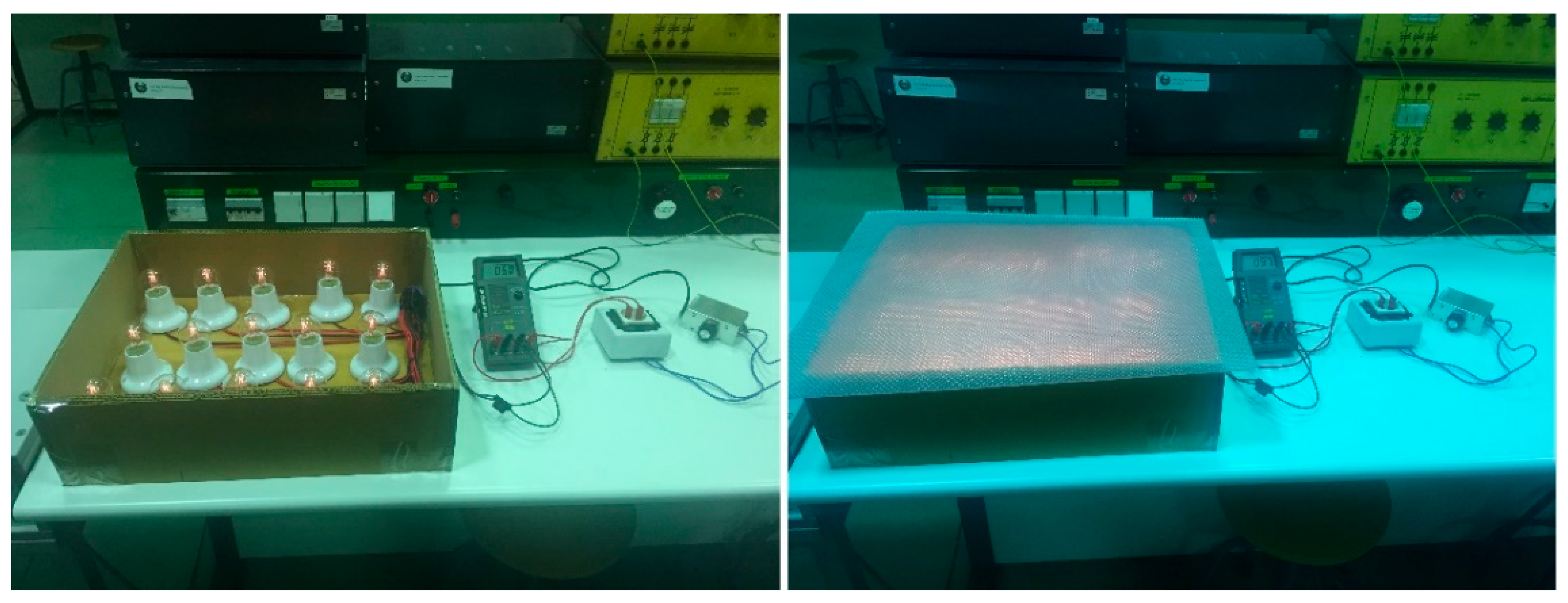
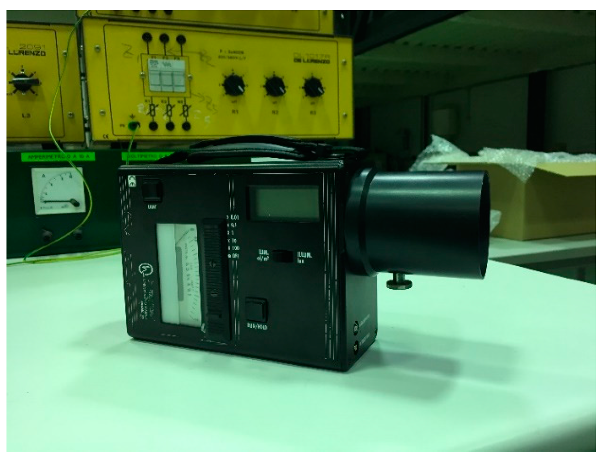
Even though this camera is not an instrument that measures luminance magnitude, it is possible to transform it into a photometer [12,18]. The information obtained in each pixel of its sensor can thus be related to the real luminance value of luminance captured in an image. To detect the luminance through any image (object image), we used a standard image of a luminous source of known luminance. Both images (object and standard images) had to be taken under the same conditions (exposure time, ISO value, aperture, camera-object distance, etc.). The luminous source consisted of a system of 15 halogen lamps arranged inside a box and covered by a diffusing screen. As shown in Figure 1, the lamps are connected in parallel to a variable power supply, which provided different luminance values. To ascertain the luminance emitted by the luminous source as a function of electrical power, we used a photometer that measures luminance (see Figure 2) and a wattmeter that measures electrical power.
2.1. Camera Calibration Procedure
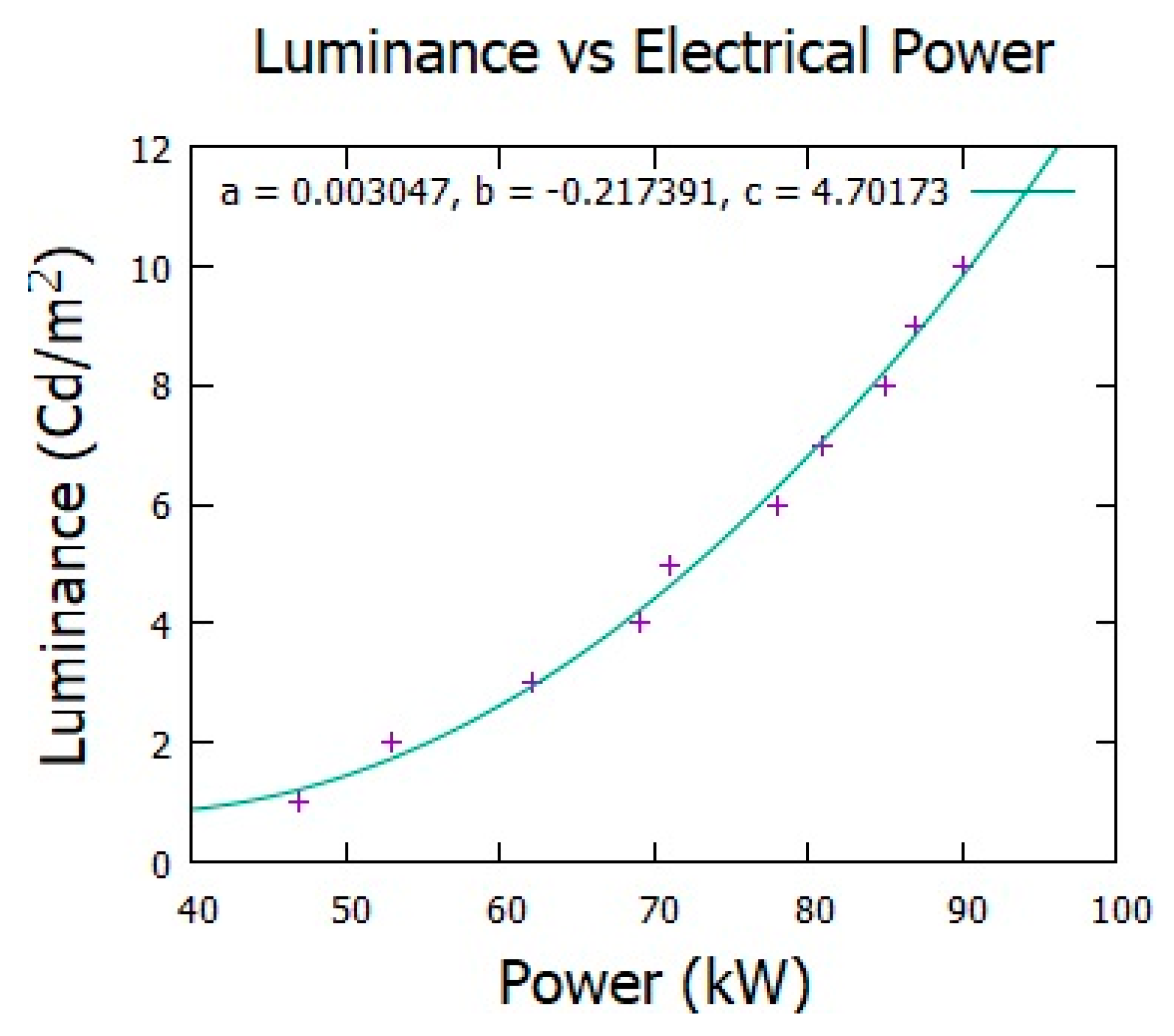
The average luminance values in street lighting range from 0.2 to 5 cd/m2, depending on the lighting class of the road. This is thus the luminance range of the pattern. To obtain this range of luminance, the lighting source is connected to a variable voltage source. Accordingly, for each voltage or power consumed (measured with a wattmeter), the system emits a certain luminance value. Figure 3 shows the relationship between the luminance emitted and the electrical power consumed. All measurements were carried out in the laboratory, after which a polynomial was formulated to fit them.
The exposure time of the camera can be adapted to the luminance level of the road, so as not to saturate the detector. For this same reason, it is also necessary to adapt the luminance of the light source (lighting pattern) to the illumination level of the road. To do this, the voltage of the source is modified where the pattern is connected. The luminance is obtained by reading the wattmeter and applying the polynomial adjustment in Figure 3.
The luminance value in cd/m2 from RGB (RGB refers to additive primary colors Red, Green and Blue, a color model used in digital cameras) images is calculated with the following expression [12,15]:
where fs is the aperture of the camera; t is the exposure time in seconds; SISO is the ISO value; K is the calibration constant; and Y is the photopic luminance value [19] calculated from the RGB color space [20] as follows:
Accordingly, the calibration procedure involves obtaining the constant K. For this purpose, we employed an image in RAW (RAW format refers to digital natives) format of the luminous pattern. The values R, G and B of each pixel were used to obtain the Y value, and the camera parameters and the known luminance of the pattern were used to deduce the calibration constant. The image processing tool for the treatment of the digital images was IRIS, a software for astrophotography [21]. This software is free for non-commercial usage and is able to process images of different formats, including photographic ones.
2.2. Method for Measuring Road Lighting
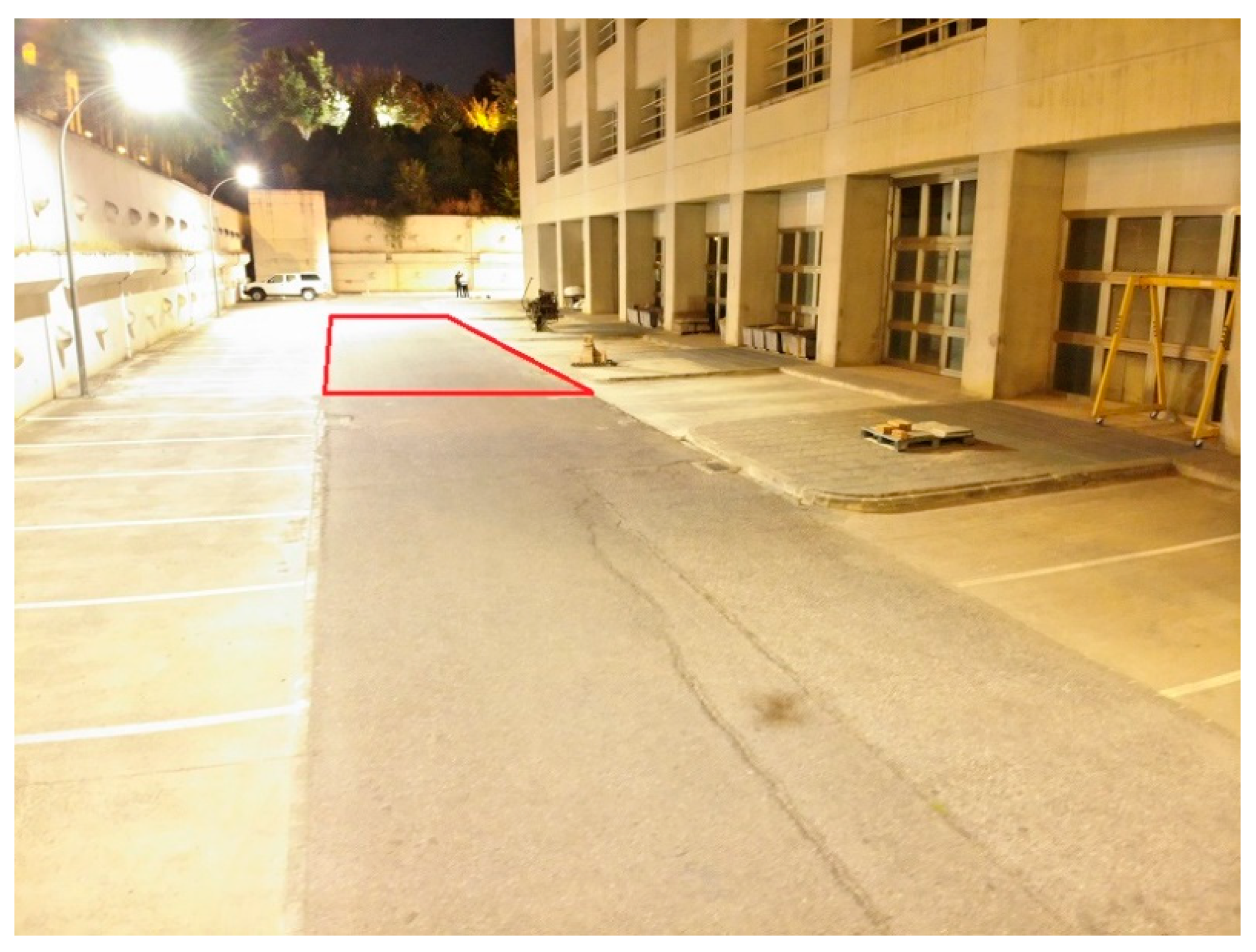
According to European standard EN 13201-3 [22,23], the average luminance of a surface must be calculated as shown in Figure 4 and Figure 5. A photometer is used to measure luminance at several points located in an area delimited by two consecutive street lights. The photometer must be at a distance of 60 m from the calculation area and at a height above the ground of 1.5 m. In our case, instead of a photometer we used the airborne camera, calibrated as described in the previous section. However, the procedure followed was the one indicated in the European standard.
2.3. Energy Efficiency of Street Lighting Installation
The energy efficiency of the lighting installation can be defined as follows:
where AT is the total illuminated surface in m2 of the street; PT is the total electrical power in watts installed, including the light sources or lamps and electrical auxiliary devices; and Xav is the average value (luminance, in cd/m2, or illuminance, in lx) on the ground. Depending on the road type, the lighting class must be based on the luminance or illuminance magnitude.
A common approach to the energy classification of public lighting installations is the use of the SLEEC (street lighting energy efficiency criterion) [5,22] as a whole system indicator, based on the efficiency of the lamp, ballast (when used) and luminaire. The formula for the SLEEC indicator (or power density indicator) depends on the photometric measurement (illuminance or luminance) used to calculate street lighting for specific road classes and is the following:
where εX is the energy efficiency of the street lighting installation; and X refers to the type of luminous parameter, based on illuminance (E) or luminance (L).
Although the definition of this indicator is still a topic of debate [24], various compatible approaches are currently available (see Table 1), in which SLEEC values are combined with the energy labelling system based on the European standard EN 13201-5. As can be observed in Table 1, the lower the consumption is, the better the energy class of the lighting installation. Therefore, the inverse of energy efficiency is a reasonable indicator that can be used to allocate an energy class to the installation.
Lighting engineering software applications base their calculations on data specifications of the street to be illuminated (i.e., dimensions, desired average illuminance, luminaire height in relation to building height, etc.). Another aspect considered is the configuration or arrangement of the installation (one-sided, two-side staggered, two-sided coupled, etc.). The main parameters obtained are the spacing between luminaires and overall uniformity.
2.4. Geographic Information System
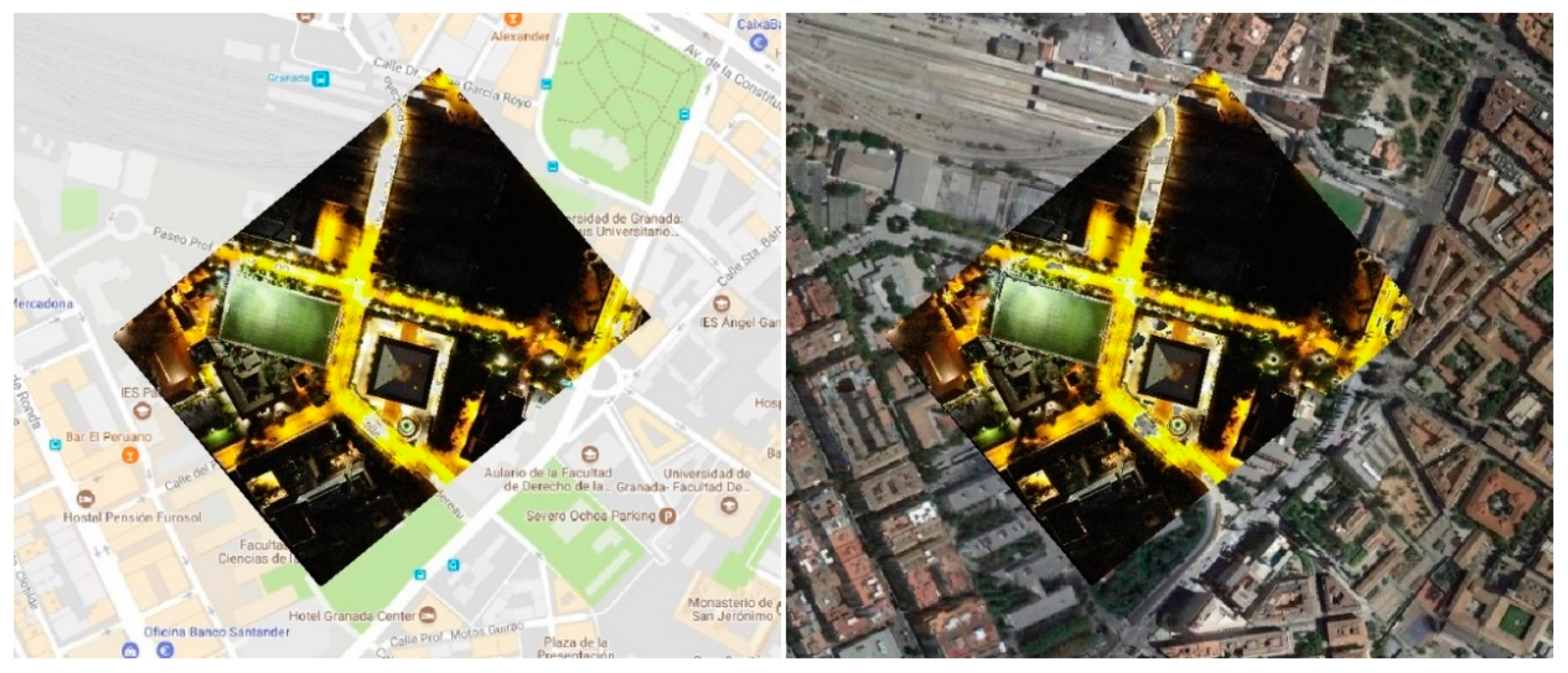
The geographic information system used in our research was QGIS [27], a free and open source software. We used QGIS to show different layers with several georeferenced attributes related to the public lighting installation. For each street or road, each layer showed the average luminance or illuminance value, uniformity (ratio of the minimum and average magnitude), position of luminaries, electrical energy consumed by luminaries and along the street, energy efficiency for each street or road, and the corresponding energy class (A, B, C, etc.). Figure 6 shows an example of one of the aerial images georeferenced with the QGIS software.
3. Results
3.1. Calibration Constant K
All images had to be captured without saturating the pixels of the camera detector. With this in mind and after several tests, we found that a good compromise was to take images with a maximum exposure time t = 1 s and ISO 1600. The luminance of the light source had to have the same order of magnitude as the lighting levels of the road. The luminance of the source when the tests were performed with the photometer (see Figure 2) was L = 1.22 cd/m2 (the light source consumed an electric power of 47 W). When Equation (1) was applied, the calibration constant of the airborne camera was K = 0.964.
3.2. Luminance Measures from Orthoimages
As mentioned in Section 2.2, the standard procedure for measuring the luminance of the road is not to place the photometer in a vertical position perpendicular to the road surface, but rather to place it horizontally 60 m from the area to be measured, and at a height of 1.5 m. Both methods do not give exactly the same result. Since the surface of the asphalt is not perfectly Lambertian [28], the reflection of the light is a combination of specular and diffuse reflection. This signifies that the light is reflected on the asphalt differently, depending on the direction.
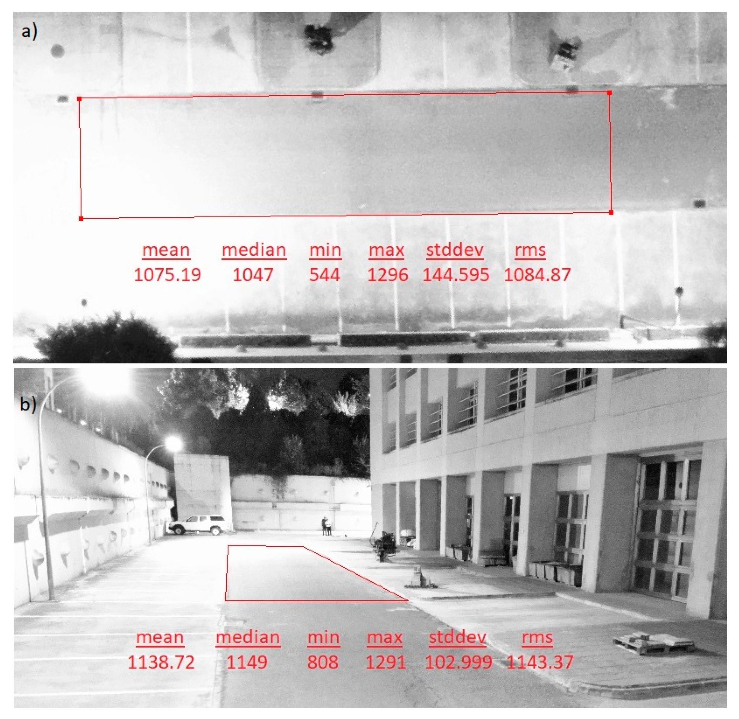
Based on this argument, we calculated the relationship between the measurement from above using an orthoimage (Figure 8) and the measurement obtained with the standard procedure (photometer in an almost horizontal position). For this purpose and as shown in Figure 9, we calculated the average luminance of all the pixels enclosed in the red box. In each image (ortho and horizontal), the statistical analysis of the calculation surface showed that that there was an approximate ratio of 1.06 between the average luminance obtained with the horizontal image and the average luminance obtained with the ortho image. This means that the luminance of ortho images had to be multiplied by a factor of 1.06 to obtain the luminance value, according to the standard road measurement procedure.
3.3. Examples of Application
The application examples were the study of lighting and energy efficiency of various streets in Deifontes, a town in southern Spain. Specifically, we studied the level of lighting, uniformity, energy consumption, energy efficiency, and energy class (A, B, C, etc.). The results indicated which improvements should be addressed to make the installation more sustainable while maintaining its functional requirements.
As a first step, the image processing software IRIS was used to transform an image in RAW format (Figure 10) into another that showed the reflected light (luminance) of the pavement, due to the information stored in each pixel. The transformation process involved obtaining the value Y for each pixel. Accordingly, Equation (2) was applied, followed by Equation (1) to obtain the vertical luminance value for each pixel. The next step involved multiplication by the correction factor 1.06 to obtain the real luminance value, according to the measurement process in the standard (Figure 11).
Any astronomical image viewer, such as IRIS or DS9 [29], can give the value of the magnitude in each pixel of the image, as well as a statistical result for all pixels in a large area. These statistical values provide average luminance or illuminance values as well as others that help to calculate lighting quality parameters, such as uniformity in a street or highway.
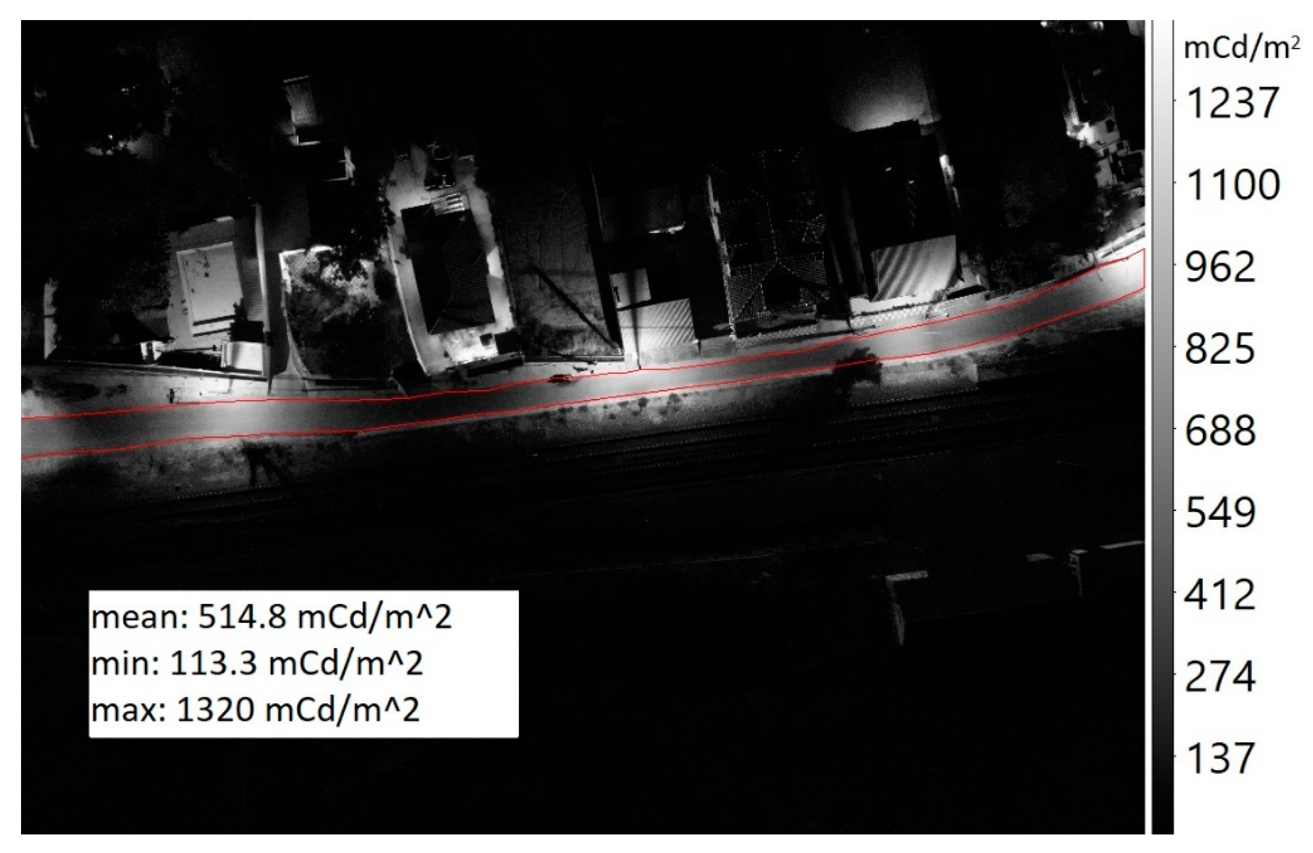
An example of this is depicted in Figure 11, where the minimum luminance (Lmin = 0.11 cd/m2) and the average luminance (Lave = 0.52 cd/m2) are obtained. These data made it possible to deduce that the luminance uniformity ( Lmin/Lave) in the street sector was 0.22. Obviously these results are not significant because the magnitude values must be calculated for the whole street and not only for one section, but in this case it is an example of the procedure described above.
There are other kinds of lighting whose magnitude of illumination is illuminance. Although luminance and illuminance are two different concepts (light emitted in one direction and light received from all directions), it is possible to relate them by taking certain margins of error into account because, in most cases, pavement characteristics are not known. However, such errors are acceptable in the field of lighting. The relationship between luminance and illuminance is shown in the following equation [15]:
where Lave and Eave are the average magnitudes in cd/m2; and lx respectively, and q0 is the average luminance coefficient. If nothing is known about the reflection properties of the pavement, a coefficient q0 = 0.07 cd/m2/lx can be applied [15].
In the following example, the procedure was simultaneously performed on several streets, captured in a single image (Figure 12). Using the previously described procedure, we calculated the luminance values in each pixel and averaged them to obtain the lighting levels of each street.
With the luminance values in each pixel, it was easy to calculate the average luminance reflected by the pavement of each street. Equation (5) was applied to obtain the average illuminance value (see Figure 13).
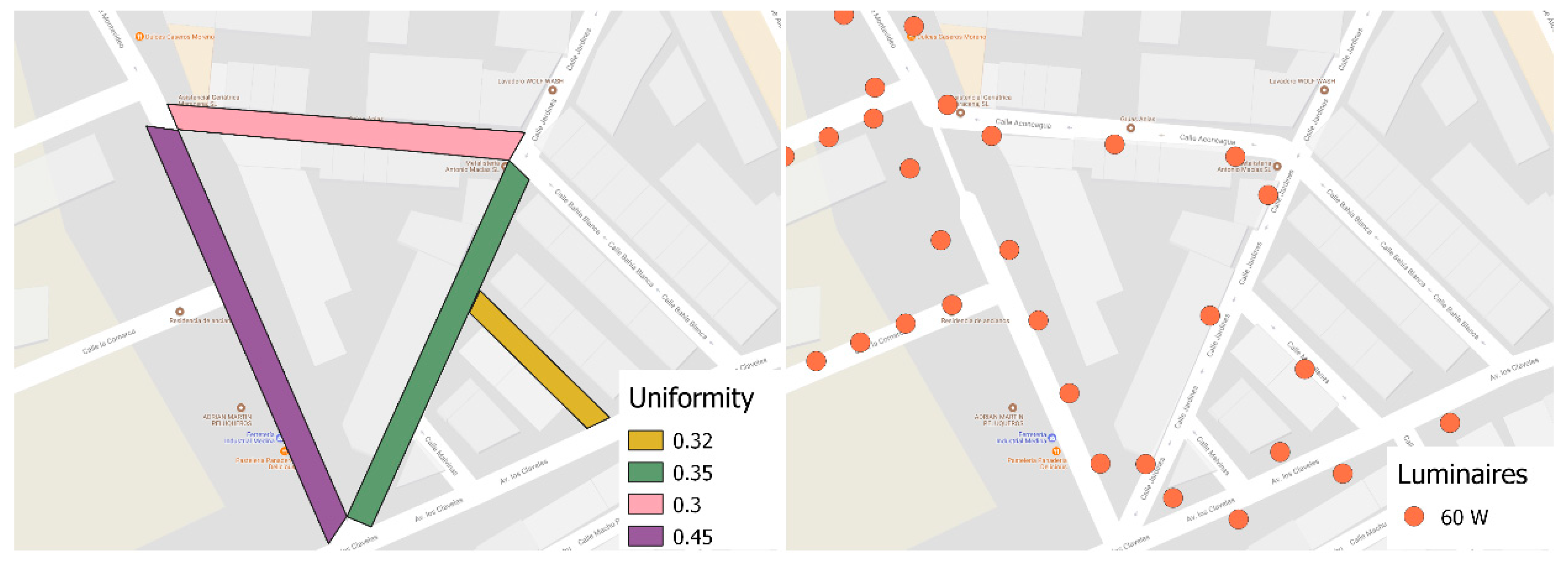
Another parameter obtained, which is directly related to the quality of street lighting, was the uniformity of the illuminance. This was possible because we knew the minimum illuminance in each street. Figure 14 shows this parameter represented in QGIS together with the position and electrical power of the luminaires.
With respect to the energy parameters, Table 2 shows the electricity consumption, the surface to be illuminated, and the average illuminance levels. Equations (3) and (4) were used to calculate the energy efficiency of the installation in each street. The electricity consumption data were obtained from the smart electric meters located in the streetlight control boxes.
Since we knew the electric power installed in a particular street, it was then possible to calculate its real electricity consumption (from data provided by the smart electric meter). This was done by applying the following equation:
where PMT is the measure of the total electrical power (provided by the smart electric meter); Pj is the known installed power in the “j” street; PT is the known installed power in all the streets connected to the smart electric meter; and PMj is the real electrical power calculated in the “j” street. This real electrical power includes the losses of the distribution lines and the actual electricity consumption of lamps and auxiliary equipment of all street lights.
4. Discussion
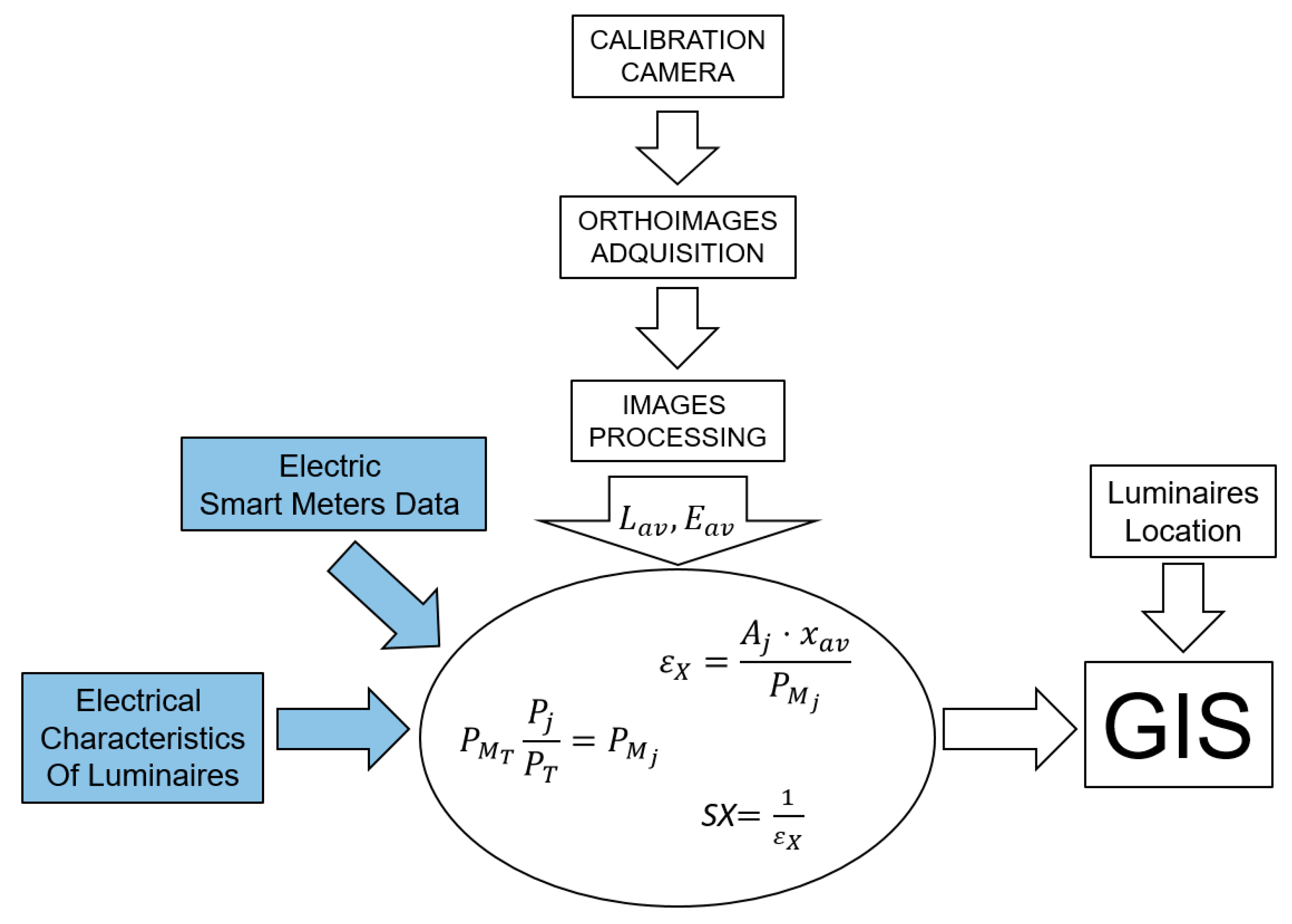
The standard procedure to obtain illumination levels of a street or road consists of measuring luminance or illuminance with photometers at street level at a few discrete points on the pavement. The standard procedure would be more precise if the number of measurement points was greater. However, this would obviously be a great deal more work. The methodology proposed (see Figure 15) allowed us to obtain the same parameters but with a greater number of measurement points (all pixels of an image or large surfaces such as roads, streets, etc.). This was accomplished by covering a larger area with a single image captured with an airborne camera. In addition, decision-making capability was improved because geographical information systems were used to implement the levels of lighting and uniformity in addition to the electrical consumption of the installation. This allowed us to calculate the energy efficiency of the installation and its energy class.
In the first example, the proposed method was applied to a small section of a street after calibrating the camera. The only information obtained was the luminance (through each pixel of the image) of the pavement. With these data we were able to calculate illuminance and uniformity. In addition, knowledge of the electrical consumption of the luminaires, the electrical energy lost by the distribution lines (electrical energy lost by the distribution lines is calculated by Boucherot’s theorem, where PLines = PTotal − PLamps. The PLamps is obtained through the manufacturer’s data sheet and PTotal through the smart electric meters located in the street light control box) and the area of the surface to be illuminated made it possible to calculate the energy efficiency of the installation. All of this information was used to ascertain whether lighting levels were optimal or whether there was an excessive consumption of electrical energy.
The second example in Figure 12 focused on pedestrian streets and streets with slow traffic in a residential area. Based on these characteristics, we deduced that the lighting class according to the CIE (CIE refers to Commission Internationale de l´Eclairage, in english International Commission of Illumination.) was P [15] (formerly known as S class). More specifically, it was P2, where the recommended illuminance level is 10–15 lx and the recommended uniformity greater than 0.3.
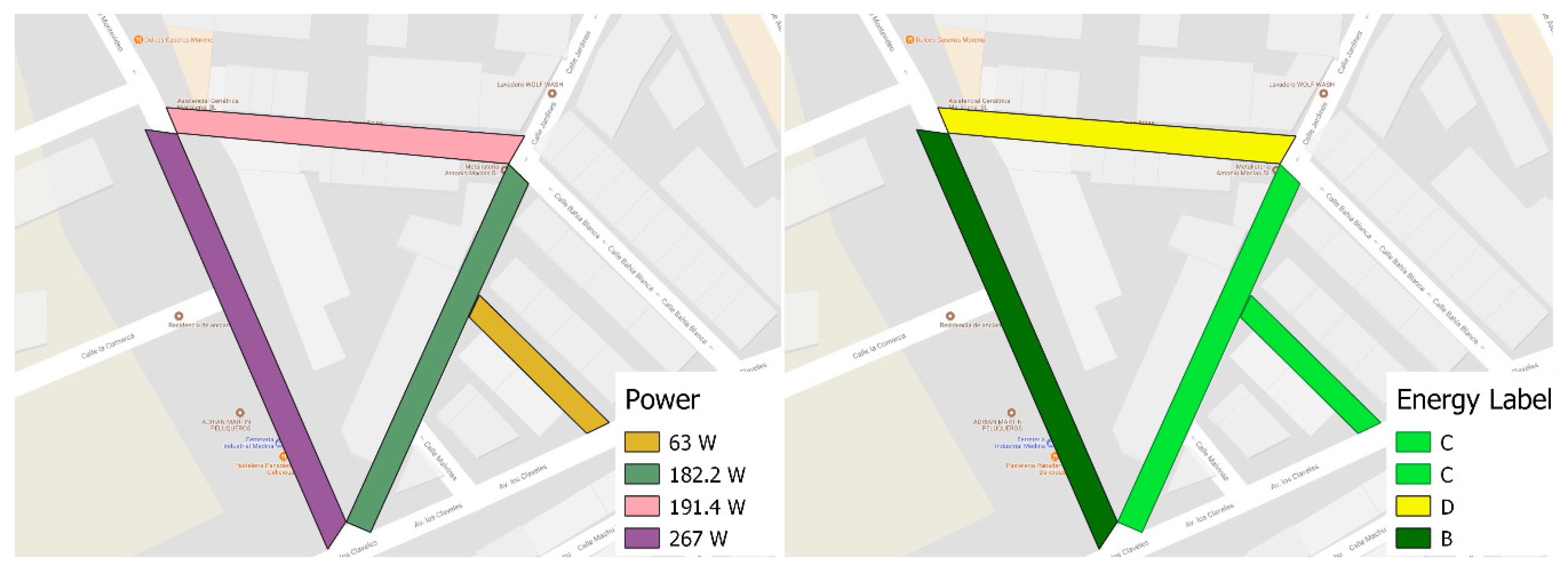
The information provided by the GIS showed that two of the four streets were correctly lit, whereas one of them (street number 2) was overlit. This clearly indicated the need to reduce either the lighting points or the electrical power of the luminaries. Of these two options, the most successful would be to reduce the electrical power of the luminaires, because removing points of light would lessen uniformity. As shown in Figure 14, the uniformity is at the limit of what is recommended by the standard. Still another reason to reduce the electrical power is the energy efficiency of the installation in that street. Figure 16 shows that its efficiency corresponds to energy class D, which means that there is room for improvement.
In contrast, street number 4 was under illuminated. Figure 13 and Figure 14 show that even though the uniformity is correct, it is very close to the minimum because there is only one luminary on the street. The energy efficiency is low but still acceptable. In this case it would be necessary to redesign the street lighting by adding one more luminaire with slightly lower electrical power. This action would improve the level of lighting and uniformity, while maintaining the same energy classification.
5. Conclusions
This research has demonstrated the viability of a method for calculating the energy efficiency of public lighting installations. It also provides a very useful tool that can be used to show their electrical and lighting properties in geographic information systems.
The electricity consumption data were obtained from smart electric meters in the streetlight control box. These meters provide information regarding the entire installation in real time. These consumption data take into account the energy consumed by lamps, auxiliary equipment, and energy losses due to the Joule effect of the distribution lines.
The geometrical distribution of the luminaires, as well as the streetlight control box, were easily georeferenced through the aerial images provided by the camera. Finally, the luminous properties were obtained by calculating the luminance emitted by the surface of the road. For this purpose, it was necessary to calibrate the airborne camera by using the image of a light source of known luminance. The calculation of the energy efficiency is almost immediate based on the electricity consumption, luminance of the road surface, and road surface dimensions.
Another important aspect is the scalability of the method. This procedure can be easily extrapolated to entire neighborhoods or cities because the only difference is the number of images needed to cover the entire metropolitan area. However, the methodology is always the same because each image is analyzed individually.
Author Contributions
Conceptualization, Methodology and Writing-Original Draft Preparation, O.R.; Investigation and Resources, E.M.-M.; Validation and Formal Analysis, D.G.-L. and F.A.-D.
Funding
This research received no external funding.
Acknowledgments
We wish to thank the city council of Deifontes (Granada) and its mayor, Francisco Abril Tenorio, for facilitating the tests carried out in the municipality. We also would like to thank Norberto Laborías Olmedo for the technical support in the Electrical Engineering Laboratory of the University of Granada.
Conflicts of Interest
The authors declare no conflict of interest.
References
- Sperber, A.N.; Elmore, A.C.; Crow, M.L.; Cawlfield, J.D. Performance evaluation of energy efficient lighting associated with renewable energy applications. Renew. Energy 2012, 44, 423–430. [Google Scholar] [CrossRef]
- Kostic, M.; Djokic, L.; Pojatar, D.; Strbac-Hadzibegovic, N. Technical and economic analysis of road lighting solutions based on mesopic vision. Build. Environ. 2009, 44, 66–75. [Google Scholar] [CrossRef]
- Kostic, M.; Djokic, L. Recommendations for energy efficient and visually acceptable street lighting. Energy 2009, 34, 1565–1572. [Google Scholar] [CrossRef]
- European Commission, DG Environment-C1. Green Public Procurement—Street Lighting and Traffics Lights. Available online: http://ec.europa.eu/environment/gpp/pdf/tbr/street_lighting_tbr.pdf (accessed on 8 August 2018).
- European Committee for Standardization (CEN). Road Lighting. Part 5: Energy Efficiency Requirements; CEN EN 13201:5; CEN: Brussels, Belgium, 2015. [Google Scholar]
- Ministry of Industry, Tourism and Trade of Spain. R.D. 1890/2008 (Regulation of Energy Efficiency in Outdoor Lighting Installations and Their Complementary Technical Instructions EA-01 to EA-07); BOE núm. 279; 19 November 2008. [Google Scholar]
- Riegel, K.W. Light Pollution: Outdoor lighting is a growing threat to astronomy. Science 1973, 30, 1285–1291. [Google Scholar] [CrossRef] [PubMed]
- Fichera, A.; Inturri, G.; LaGreca, P.; Palermo, V. A model for mapping the energy consumption of buildings, transport and outdoor lighting of neighbourhoods. Cities 2016, 55, 49–60. [Google Scholar] [CrossRef]
- Sedziwy, A.; Kotulski, L. Multi-agent system supporting automated GIS-based photometric computations. Procedia Comput. Sci. 2016, 80, 824–833. [Google Scholar] [CrossRef]
- Ekrias, A.; Eloholma, M.; Halonen, L.; Song, X.J.; Zhang, X.; Wen, Y. Road lighting and headlights: Luminance measurements and automobile lighting simulations. Build. Environ. 2008, 43, 530–536. [Google Scholar] [CrossRef]
- Zhou, H.; Pirinccioglu, F.; Hsu, P. A new roadway lighting measurement system. Transp. Res. Part C Emerg. Technol. 2009, 17, 274–284. [Google Scholar] [CrossRef]
- Vaaja, M.T.; Kurkela, M.; Virtanen, J.P.; Maksimainen, M.; Hyyppä, H.; Hyyppä, J.; Tetri, E. Luminance-corrected 3D point clouds for road and street environments. Remote Sens. 2015, 7, 11389–11402. [Google Scholar] [CrossRef]
- Wüller, D.; Gabele, H. The usage of digital cameras as luminance meters. Proc. SPIE 2007, 6502, 65020U. [Google Scholar]
- Xu, Y.; Knudby, A.; Côté-Lussier, C. Mapping ambient light at night using field observations and high-resolution remote sensing imagery for studies of urban environments. Build. Environ. 2018, 145, 104–114. [Google Scholar] [CrossRef]
- International Commission on Illumination (CIE). Lighting of Roads for Motor and Pedestrian Traffic; CIE Public 115; CIE: Vienna, Austria, 2010. [Google Scholar]
- Beccali, M.; Bonomolo, M.; Ciulla, G.; Galatioto, A.; Lo Brano, V. Improvement of energy efficiency and quality of street lighting in South Italy as an action of Sustainable Energy Action Plans. The case study of Comiso (RG). Energy 2015, 92, 394–408. [Google Scholar] [CrossRef] [Green Version]
- Carli, R.; Dotoli, M.; Pellegrino, R. A decision-making tool for energy efficiency optimization of street lighting. Comput. Oper. Res. 2018, 96, 223–235. [Google Scholar] [CrossRef]
- Hiscocks, P.D.; Eng, P. Measuring Luminance with a Digital Camera: Case History. Available online: http://www.ee.ryerson.ca:8080/~phiscock/astronomy/light-pollution/luminance-case-history.pdf (accessed on 18 August 2018).
- CIE. Commission Internationale de l’Eclairage Proceedings, 1924; Cambridge University Press: Cambridge, UK, 1926. [Google Scholar]
- Süsstrunk, S.; Buckley, R.; Swen, S. Standard RGB Color Spaces. In Proceedings of the IS&T/SID’s 7th Color Imaging Conference, Scottsdale, AZ, USA, 16–19 November 1999; pp. 127–134. [Google Scholar]
- Spectroscopy, CCD and Astronomy. Available online: http://www.astrosurf.com/buil/iris-software.html (accessed on 28 August 2018).
- European Committee for Standardization (CEN). Road Lighting. Part 3: Calculation of Performance; CEN EN 13201:3; CEN: Brussels, Belgium, 2003. [Google Scholar]
- International Commission on Illumination (CIE). Road Lighting Calculations; CIE Public 140; CIE: Vienna, Austria, 2000. [Google Scholar]
- Domke, K.; Brebbia, C.A. Light in Engineering, Architecture and Environment; WIT Press: Southampton, UK, 2011; pp. 135–137. ISBN 978-1-84564-550-2. [Google Scholar]
- Rabaza, O.; Gómez-Lorente, D.; Pérez-Ocón, F.; Peña-García, A. A simple and accurate model for the design of public lighting with energy efficiency functions based on regression analysis. Energy 2016, 107, 831–842. [Google Scholar] [CrossRef]
- King, B.; Bridger, G. Review of Road Lighting Design Classification System. 2015. Available online: http://www.energyrating.gov.au/document/report-review-road-lightingdesign-classification-system (accessed on 16 August 2018).
- QGIS. Available online: https://www.qgis.org/en/site/ (accessed on 10 September 2018).
- Alamdarlo, M.N.; Hesami, S. Optimization of the photometric stereo method for measuring pavement texture properties. Measurement 2018, 127, 406–413. [Google Scholar] [CrossRef]
- SAOImage DS9. Available online: http://ds9.si.edu/site/Home.html (accessed on 10 September 2018).
Figure 1.
Source used as a luminance pattern. The left image shows the lamp distribution inside the box connected to the wattmeter and a variable power supply. The right image shows the screen diffuser over the box.
Figure 1.
Source used as a luminance pattern. The left image shows the lamp distribution inside the box connected to the wattmeter and a variable power supply. The right image shows the screen diffuser over the box.

Figure 2.
Hagner universal photometer S3 used to measure luminance.

Figure 3.
Relationship between the luminance emitted by the standard luminous source as a function of the electrical power consumed and the coefficients of a second-order polynomial (ax2 + bx + c) fit to the measured values.
Figure 3.
Relationship between the luminance emitted by the standard luminous source as a function of the electrical power consumed and the coefficients of a second-order polynomial (ax2 + bx + c) fit to the measured values.

Figure 4.
Field of calculation for carriage luminance, where (a) is the side-view and (b) the top-view.
Figure 4.
Field of calculation for carriage luminance, where (a) is the side-view and (b) the top-view.

Figure 5.
Digital image in which the calculation area of average luminance is indicated by a red frame. According to the standard procedure the camera is located at a distance of 60 m from the calculation area and at a height of 1.5 m.
Figure 5.
Digital image in which the calculation area of average luminance is indicated by a red frame. According to the standard procedure the camera is located at a distance of 60 m from the calculation area and at a height of 1.5 m.

Figure 6.
Aerial image taken with an airborne camera. The image was georeferenced with QGIS.

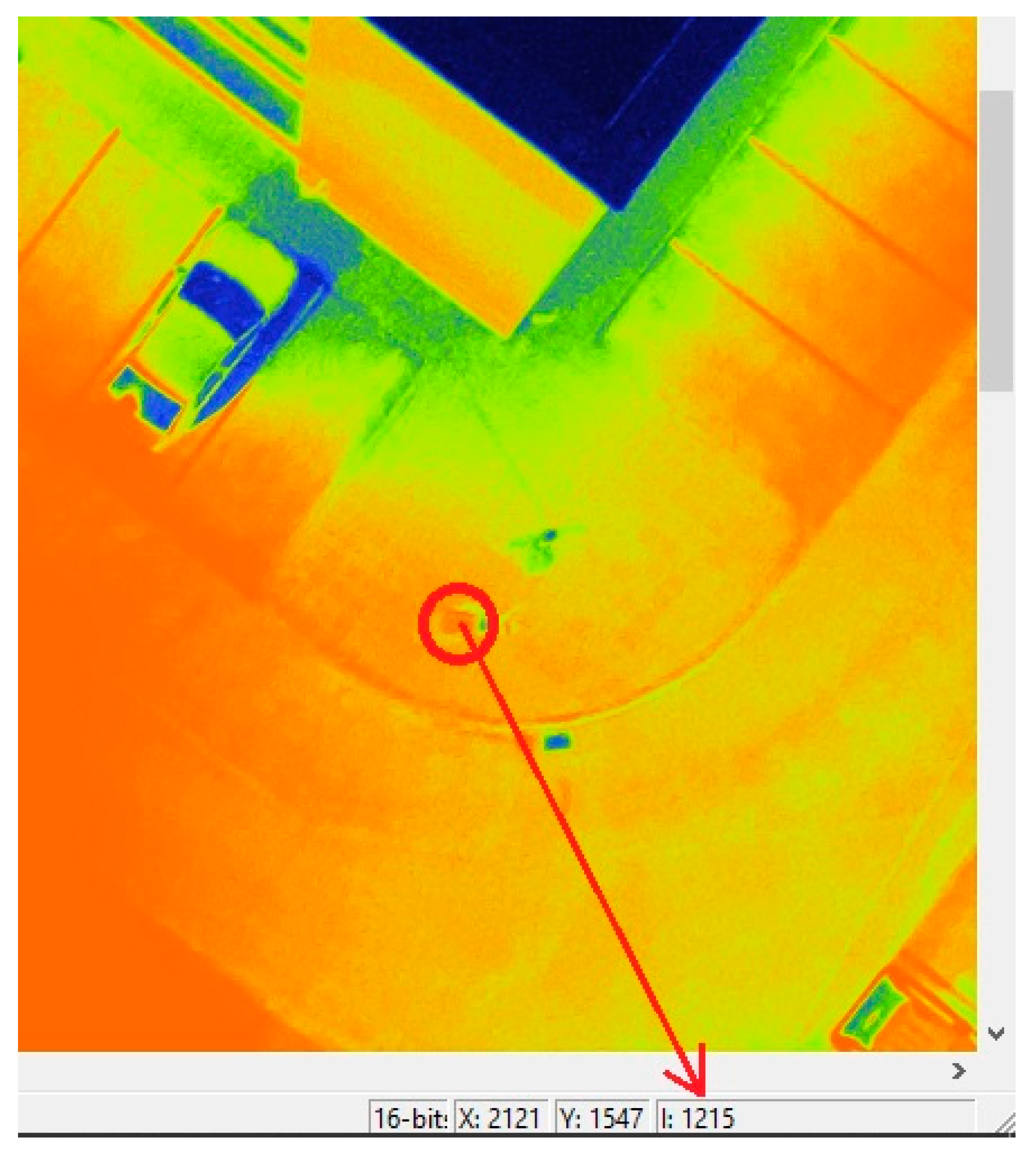
Figure 7.
The image processing tool IRIS gives the luminance values at mCd/m2 emitted by the ground surface. The red circle depicts the position of the light source and the arrow shows the relative coordinates in pixels (X = 2121, Y = 1547) and the luminance value L = 1215 mCd/m2.
Figure 7.
The image processing tool IRIS gives the luminance values at mCd/m2 emitted by the ground surface. The red circle depicts the position of the light source and the arrow shows the relative coordinates in pixels (X = 2121, Y = 1547) and the luminance value L = 1215 mCd/m2.

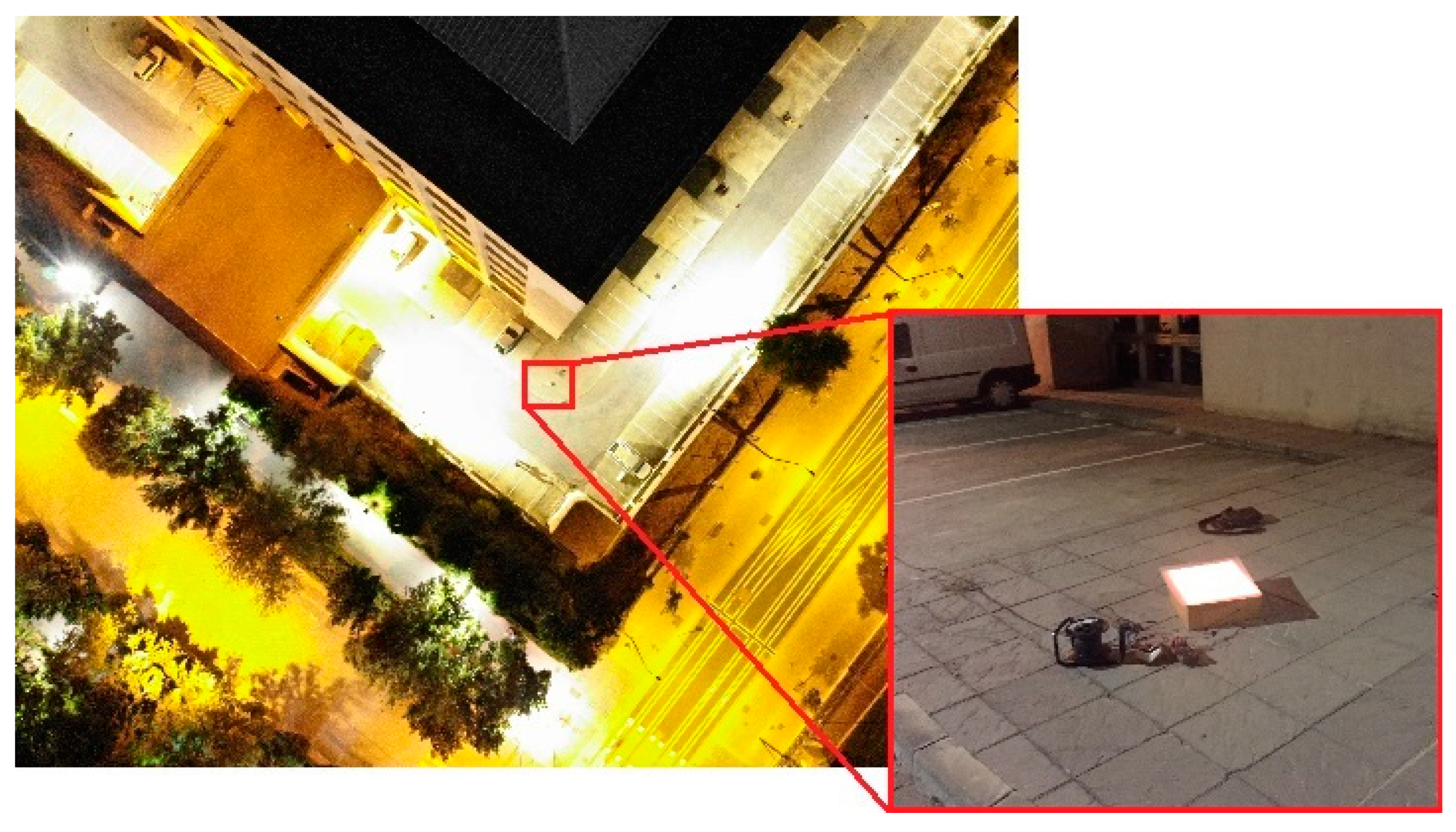
Figure 8.
Aerial photo image of the area where the light source and the wattmeter were placed. Depending on the electrical power demanded by the source, we were able to deduce the luminance emitted.
Figure 8.
Aerial photo image of the area where the light source and the wattmeter were placed. Depending on the electrical power demanded by the source, we were able to deduce the luminance emitted.

Figure 9.
Average luminance and other statistical values (at mCd/m2) of the calculation area from the aerial image or orthoimage (a) and the image where the standard procedure was applied (b).
Figure 9.
Average luminance and other statistical values (at mCd/m2) of the calculation area from the aerial image or orthoimage (a) and the image where the standard procedure was applied (b).

Figure 10.
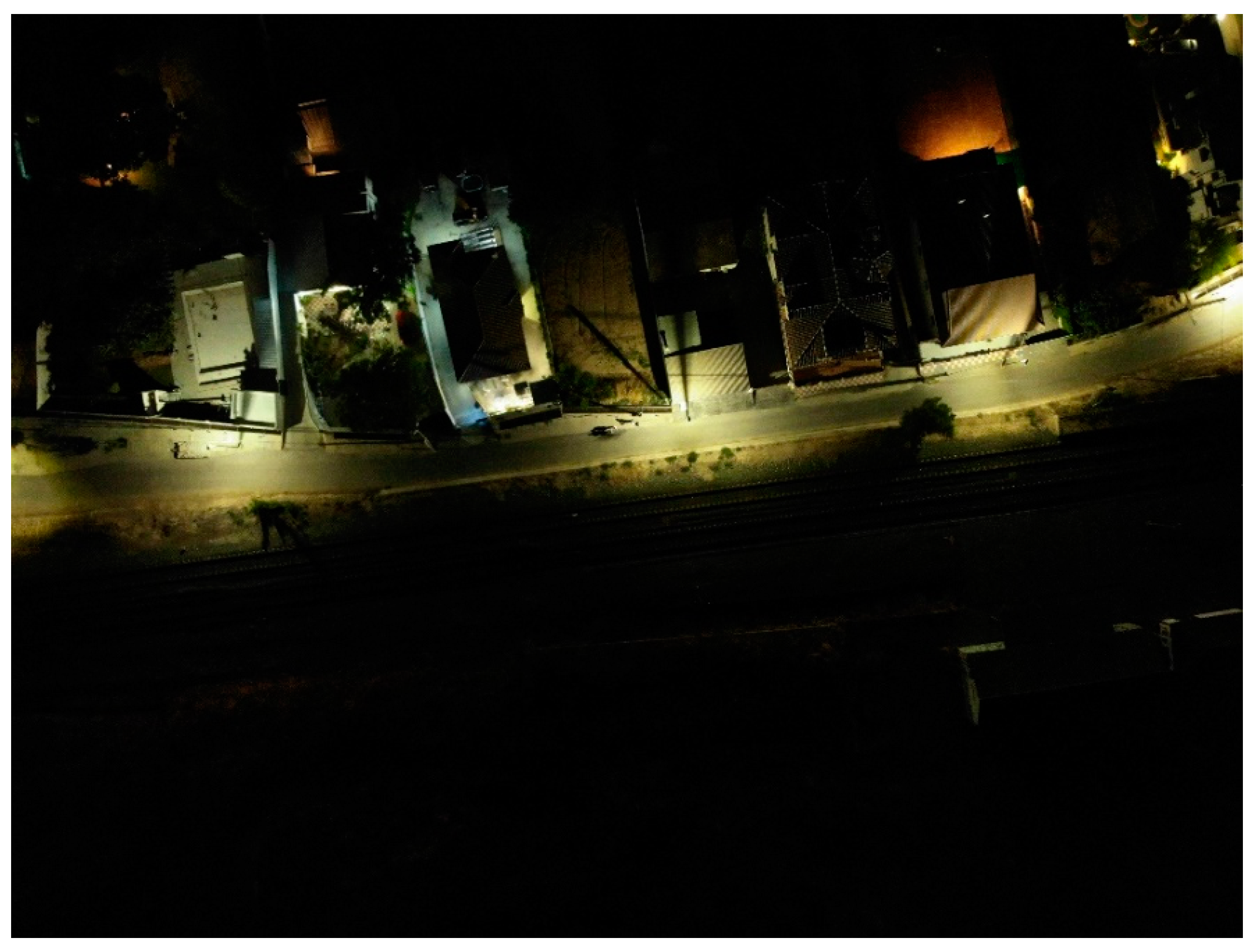
Orthoimage of a street obtained by the airborne camera. The image is in RAW format and had not yet been treated with the image processing software.
Figure 10.
Orthoimage of a street obtained by the airborne camera. The image is in RAW format and had not yet been treated with the image processing software.

Figure 11.
Orthoimage treated with IRIS software and visualized with DS9. The figure shows the luminance values for each pixel and a statistical analysis of the corresponding lighting values of the road (only for the calculation area in the red polygon).
Figure 11.
Orthoimage treated with IRIS software and visualized with DS9. The figure shows the luminance values for each pixel and a statistical analysis of the corresponding lighting values of the road (only for the calculation area in the red polygon).

Figure 12.
Aerial image in RAW (left) and georeferenced (right) format

Figure 13.
Average luminance (left) and illuminance (right) levels of some streets.

Figure 14.
Illuminance uniformity (left) and luminaires position (right).

Figure 15.
Diagram of the stages of the methodology. The blue boxes indicate the information provided by the local city council.
Figure 15.
Diagram of the stages of the methodology. The blue boxes indicate the information provided by the local city council.

Figure 16.
Power consumed in each street (left) and energy class (right).


Table 1.
Energy efficiency classification of street lighting installations according to the street lighting energy efficiency criterion (SLEEC) indicator [25].
Table 1.
Energy efficiency classification of street lighting installations according to the street lighting energy efficiency criterion (SLEEC) indicator [25].
| Energy Class | SE (W/lx∙m2) | SL (W/cd) |
|---|---|---|
 | 0.000–0.014 | 0.00–0.21 |
| 0.015–0.024 | 0.22–0.36 | |
| 0.025–0.034 | 0.37–0.51 | |
| 0.035–0.044 | 0.52–0.66 | |
| 0.045–0.054 | 0.67–0.81 | |
| 0.055–0.064 | 0.82–0.96 | |
| 0.065–0.074 | 0.97–1.11 |
Table 2.
Lighting and electrical parameters of each street used to calculate the energy efficiency of the installation.
Table 2.
Lighting and electrical parameters of each street used to calculate the energy efficiency of the installation.
| Street | Pavement Area (m2) | Electrical Power (W) | Illuminance (lx) | SE (W/lx/m2) | Energy Class |
|---|---|---|---|---|---|
| 1 | 890 | 267.0 | 15 | 0.020 | B |
| 2 | 290 | 191.4 | 16.5 | 0.040 | D |
| 3 | 460 | 182.2 | 12 | 0.033 | C |
| 4 | 250 | 63.0 | 9 | 0.028 | C |
© 2018 by the authors. Licensee MDPI, Basel, Switzerland. This article is an open access article distributed under the terms and conditions of the Creative Commons Attribution (CC BY) license (http://creativecommons.org/licenses/by/4.0/).
Share and Cite
MDPI and ACS Style
Rabaza, O.; Molero-Mesa, E.; Aznar-Dols, F.; Gómez-Lorente, D. Experimental Study of the Levels of Street Lighting Using Aerial Imagery and Energy Efficiency Calculation. Sustainability 2018, 10, 4365. https://doi.org/10.3390/su10124365
AMA Style
Rabaza O, Molero-Mesa E, Aznar-Dols F, Gómez-Lorente D. Experimental Study of the Levels of Street Lighting Using Aerial Imagery and Energy Efficiency Calculation. Sustainability. 2018; 10(12):4365. https://doi.org/10.3390/su10124365
Chicago/Turabian StyleRabaza, Ovidio, Evaristo Molero-Mesa, Fernando Aznar-Dols, and Daniel Gómez-Lorente. 2018. "Experimental Study of the Levels of Street Lighting Using Aerial Imagery and Energy Efficiency Calculation" Sustainability 10, no. 12: 4365. https://doi.org/10.3390/su10124365
Note that from the first issue of 2016, this journal uses article numbers instead of page numbers. See further details here.