Exploring the Factors Controlling Nighttime Lights from Prefecture Cities in Mainland China with the Hierarchical Linear Model


1
School of Remote Sensing and Information Engineering, Wuhan University, Wuhan 430072, China
2
School of Architecture and Civil Engineering, Xiamen University, Xiamen 361005, China
*
Author to whom correspondence should be addressed.
Remote Sens. 2020, 12(13), 2119; https://doi.org/10.3390/rs12132119
Submission received: 20 May 2020
/
Revised: 25 June 2020
/
Accepted: 30 June 2020
/
Published: 2 July 2020
(This article belongs to the Special Issue Remote Sensing of Nighttime Observations)
Abstract
:Nighttime light data have been proven to be valuable for socioeconomic studies. However, they are not only affected by anthropogenic factors but also by physical factors, and previous studies have rarely examined these diverse variables in a systematic way that explains differences in nighttime lights across different cities. In this paper, hierarchical linear models at two levels of city and province were developed to investigate the nighttime lights effect on cross-level factors. An experiment was conducted for 281 prefecture cities in Mainland China using orbital satellite data in 2016. (1) There exist significant differences among city average lights, of which 49.9% is caused at the provincial level, indicating the factors at the provincial level cannot be ignored. (2) Economy-energy-infrastructure and demography factors have a significant positive lights effect. Meanwhile, industry-information and living-standard factors at the provincial level can further significantly increase these differences by 18.30% and 29.01%, respectively. (3) The natural-greenness factor displayed a significant negative lights effect, and its interaction with natural-ecology will continue to decrease city lights by 11.99%. However, artificial-greenness is an unreliable city-level factor explaining lights variations. (4) As for the negative lights effect of elevation and latitude, these become significant in a multivariate context and contribute lights indirectly. (5) The two-level hierarchical linear models are statistically significant at the level of 10%, and compared with the null model, the explained variances on city lights can be improved by 70% at the city level and 90% at the provincial level in the final mixed effect model.
1. Introduction
Human activities and their footprints on earth can be clearly observed in space through nighttime light imagery [1,2]. The widely used remotely sensed nighttime data are provided by the Defense Meteorological Satellite Program (DMSP)’s Operational Linescan System (OLS) and Suomi National Polar-orbiting Partnership (NPP) Satellite’s Visible Infrared Imaging Radiometer Suite (VIIRS) [3,4]. DMSP data have been used to map the global nighttime lights for many years [5], and the basic product is the annual cloud-free stable lights imagery, which is freely available from 1992 to 2013. However, DMSP data have been reported with several drawbacks. For instance, they have a relatively low spatial resolution, which could lead to unreliable estimation of city lights. They are recorded with a relatively low radiometric resolution, which could lead to saturation in urban areas and overglow near the city boundary [6]. Recently, VIIRS data have been released by the Earth Observation Group spanning from 2011. Compared to DMSP data, they appear to be much more promising, for instance, they have a finer spatial resolution of around 500 m, a larger number of 22 spectral bands, and a better radiometric resolution of 14 bits [7]. Importantly, they are radiometrically calibrated onboard, and they seem to be less affected by the problem of over-saturation in urban areas owing to an extended spectral coverage (from 500 nm to 900 nm) in the day/night band (DNB) [8,9]. Thus, VIIRS data can probably be regarded as a better proxy for anthropogenic development ([5,10]).
Extensive studies have demonstrated a variety of relationships between nighttime lights and socioeconomic or demographic factors [4,8,11,12,13,14,15,16,17,18,19,20], which means that nighttime lights variations in space can be adequately explained or controlled by these factors. However, previous studies were conducted mainly to explain the spatial differences of lights in terms of GDP, population, or electricity at the country or provincial level using DMSP data [4,11]. With the availability of VIIRS data, most studies have been focused on examining factors explaining lights differences at different levels. Shi et al. [8] showed that VIIRS lights are correlated better with GDP or electricity than the ones from DMSP at both provincial and city levels [8]. Ma et al. [12] reported high responses of VIIRS lights to the population, GDP, electric consumption, road area at the city level, and passenger traffic at the airport level. Kyba et al. [13] examined the relationship between VIIRS lights and population, and the differences were compared for cities in the USA and Germany. Zhao et al. [14] showed that the sum of lights has a more significant relationship with economic variables than other lights indices. Besides, recent studies [15,20] indicated that VIIRS lights are highly correlated with human activity intensity derived from social media data at the pixel level or city level. Interestingly, Chen and Nordhaus [17] suggested that VIIRS lights provide a better prediction for cross-sectional GDP than time-series GDP, and Sun et al. [16] revealed a positive correlation between VIIRS lights and land surface temperature, which considered natural ecological factors.
The studies above explored their relationships using different regression models. Most studies adopted a simple linear regression model [8,12,13,17,18,20], although there are a few studies using a quantile regression [21], a quadratic polynomial regression [14], a step-wise regression [22], a geographical weighted regression [15], or even a mixed effect regression [23]. Statistical relationships change with variables, space, and time [24], implying the complexity of land surface and the variety of human activities [25]. Furthermore, only a small number of variables were considered in these models, which might give limited explanations on lights variations. This is because nighttime lights can be affected not only by factors related to socioeconomic, infrastructure, and natural ecology but also by the interactions between these factors. Specifically, Levin and Zhang [1] developed a generalized multivariate linear model to explain their spatial variations at the city level using two groups of variables including socioeconomic variables (GDP per capita, population density, et al.) and physical variables (Normalized Difference Vegetation Index (NDVI), latitude, et al.), and their model can explain more than 45% of lights variations. Nonetheless, it did not consider the interactive light effect of cross-level variables, which is mainly due to the nested structure of anthropogenic development in space [26]. In fact, current studies were focused mainly on associating nighttime lights with characteristics of the spatial unit at one single level. However, the variations may exist not only between cities but also within a broader spatial extent, i.e., the overall development of a city being influenced by the region where it is located. The interactive effect between a city and where it is situated has not been fully investigated in the literature. Specifically, with the reform and opening up of Mainland China, the speed and intensity of urban development are unevenly distributed in different provinces, which may also shed a non-trivial impact on nighttime lights. For instance, Du and Yu [27] reported that provincial economic factors have impact on nighttime lights of urban areas.
In addition, hierarchical linear models have been used to model the multi-level relationship of factors in many fields [28,29,30]. However, there are rarely studies using this method to examine the factors controlling nighttime lights. Therefore, this study aims to develop hierarchical linear models at two levels of city and province for a systematic and comprehensive analysis of a variety of anthropogenic and physical factors of nighttime lights for 281 prefecture cities in Mainland China, and particularly, it intends to explore the nighttime lights effect of cross-level factors. As aforementioned, city lights are not only relevant to the city’s anthropogenic and physical variables but are also affected by the diverse variables in the province where they are located. In other words, there are significant differences in the nighttime lights of different provinces [31]. This is highly consistent with the hierarchical (nested) structure of the administrative system in Mainland China [32]. Thus, the main contributions of this study are focused on the following two aspects, which are also the major differences from previous studies. (1) We conducted a systematic analysis of the nighttime lights effect of cross-level factors, which are derived from 12 city-level variables and 16 province-level variables. It is rarely reported in the literature by integrating all these uncorrelated factors into the same analytic framework. (2) We developed a two-level hierarchical linear model, which covers four types of models including the unconditional means model, random intercept model, mixed-effect model with one single city-level factor, and the mixed-effect model with all city-level factors. The results suggested the superiority of our model, and they can enhance our understanding of the mechanism underlying remote sensing of nighttime light, which will be valuable for socioeconomic studies.
The rest of this paper is organized as follows. In Section 2, we describe the study area, the datasets, and the derivation of uncorrelated factors. In Section 3, we propose the two-level hierarchical linear model. In Section 4, we analyze the experimental results. Discussions and limitations are presented in Section 5. Conclusions are drawn in Section 6.
2. The Study Area, Datasets and their Preprocess
2.1. Description of the Study Area
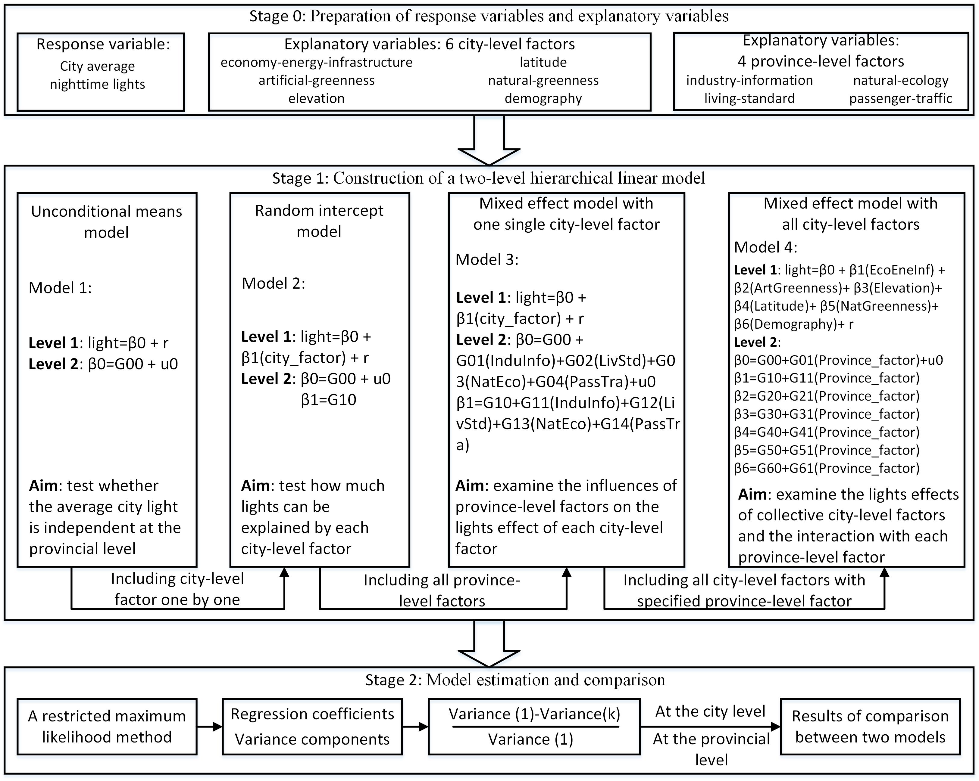
China is located in eastern Asia, which has an unbalanced urban development for cities in different regions. The administrative system has a hierarchical (nested) structure at different levels [32], which is composed of 2846 counties, 333 prefecture cities, and 34 provinces as reported in 2016. This hierarchical structure indicates that cities in developed provinces tend to have more opportunities for development than cities in underdeveloped provinces. In this study, a total number of 281 prefecture cities are selected from 30 provinces due to the unavailability of data in Tibet and the inconsistencies of statistics in Taiwan, Hong Kong, and Macau. As shown in Figure 1, the selected prefecture cities are distributed unevenly in space with different levels of average nighttime lights, and they account for 92.37% of the population and 91.62% of the GDP in Mainland China in 2016. Statistically, cities located in the southeastern division of the Aihui-Tengchong Line constitute around 90.76% of the total lights, while cities in the northwestern division occupy only 9.24%. This finding roughly coincides with population distribution in the two divisions, where 93% of population is in the southeast and only 7% is in the northwest. Thus, it is reasonable to select the 281 prefecture cities, and they can reflect the situation in Mainland China.
2.2. The Datasets
2.2.1. VIIRS Nighttime Light Dataset
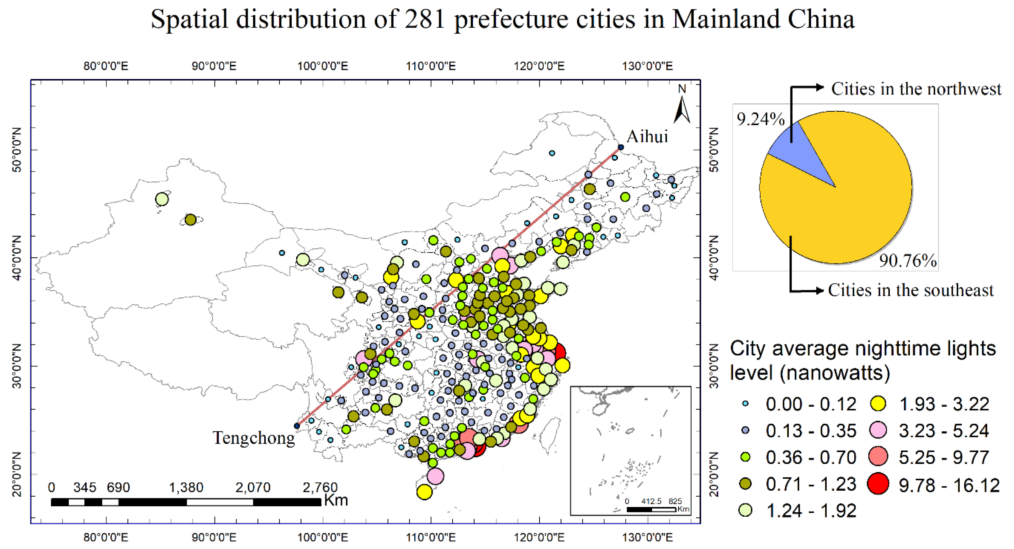
The VIIRS nighttime light dataset in 2016 was downloaded freely from the official site (source: http://ngdc.noaa.gov/eog/), which belongs to the version 1 series of annual average radiance composites spanning the globe from 75 N latitude to 65 S. It has been preprocessed to remove temporal lights and background non-light values. It is composed of 6 tiles, and they are cut at the equator, and each span 120 degrees of latitude. In this study, we have downloaded the annual cloud-free composite of tile 3 as it covers the entire study area, which is used to calculate the average lights levels of prefecture cities. Besides, it was further clipped by the boundary of Mainland China. As shown in Figure 2a, we can see that there is a wide range of pixel values from 0 to 1280.79, which indicates that it can be less affected by the typical over-saturation problem in urban center.
2.2.2. The Ancillary Datasets
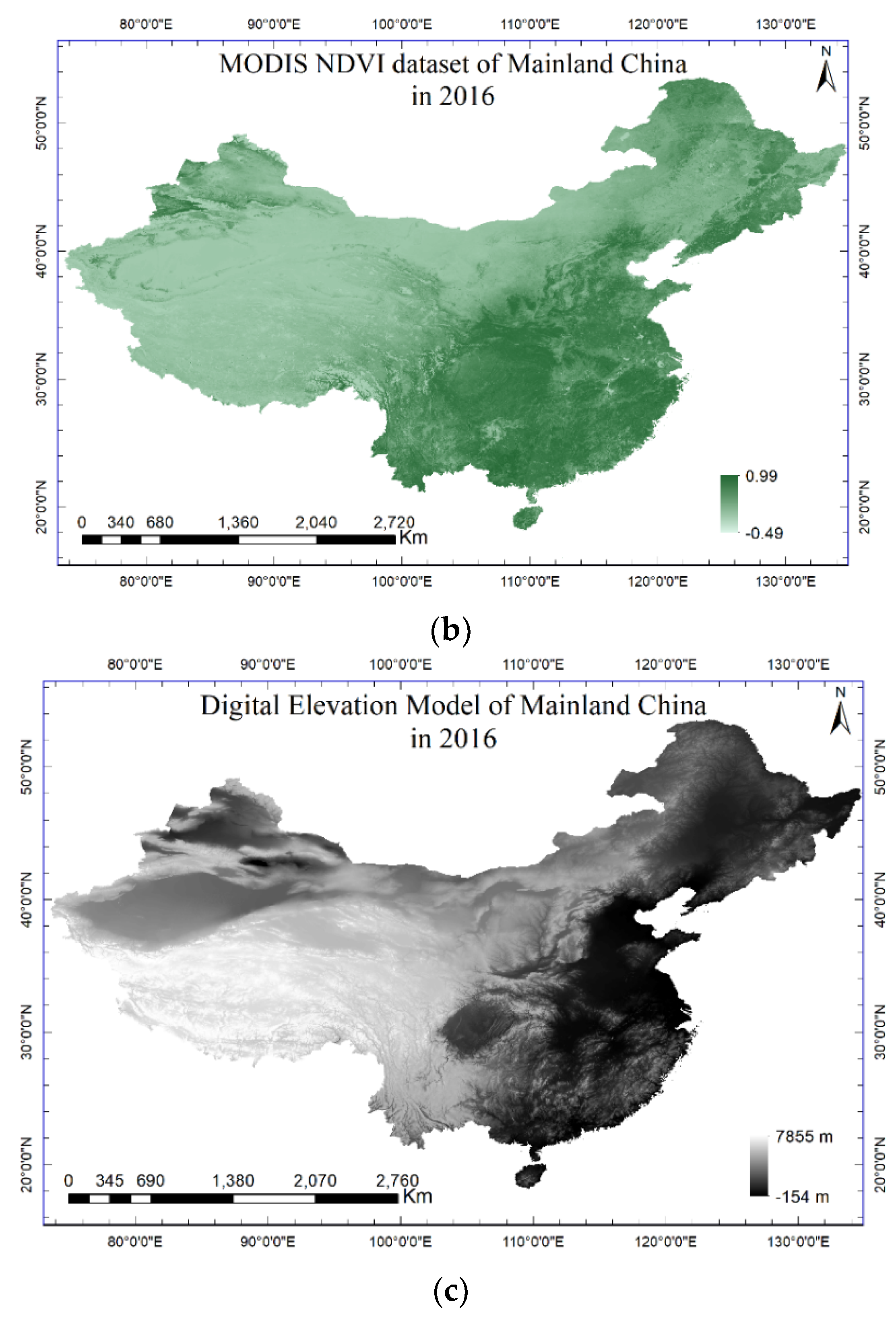
The Normalized Difference Vegetation Index (NDVI) dataset was downloaded for free from the platform of the Computer Network Information Center at the Chinese Academy of Science (http://www.gscloud.cn). It is a composite product (MODND1T) produced for China in 2016 at the spatial resolution of 500 m. NDVI is calculated using the blue, red, and near-infrared reflectivity bands of satellite imageries, and thus, it can reflect the characteristics of vegetation conditions. In this study, it was further clipped by the boundary of Mainland China. As shown in Figure 2b, there are around 99.31% of pixels with values larger than 0, and there are only 0.69% of pixels with values less than 0, which are mostly covered by lakes and snowy peaks.
The Digital Elevation Model (DEM) dataset was obtained from the China Historical Geographic Information System (www.people.fas.harvard.edu/~chgis/), produced by a collaboration between Harvard University and Fudan University, which provides a database for scholarly and scientific research. In this study, we have downloaded the DEM data of China in 2016, which is based on GTOPO-30 data from USGS and at the spatial resolution of 1000 m. It was further clipped by the boundary of Mainland China. As shown in Figure 2c, we can roughly see that developed regions in the southeast tend to have lower values of elevation than underdeveloped regions in the northwest. In this respect, elevation might be indirectly related to nighttime light.
The statistical yearbook dataset in 2016 was provided for free by the CEInet Statistics Database, for academic use only (www.db.cei.cn/page/Default.aspx), which is an authoritative organization under the National Information Center of China. In this study, it provided basic socioeconomic information for the prefecture cities and the corresponding provinces.
2.3. Selection of Variables and Derivation of Factors
2.3.1. Selection of Variables
Based on the datasets, we obtained a diverse number of variables, as shown in Table 1, namely 12 city-level variables and 16 province-level variables. These variables were selected because they might be related to nighttime lights and are available in our study area.
- Variables at the city level: GDP, GDP per capita, population, population density, total electric consumption, road area, urban built-up area, personal city green space area, and personal urban green coverage area. These variables were obtained from the statistical yearbook dataset. The personal city green space area denotes the total area of various types of green space divided by the population, and a certain type of green space has to satisfy the strict minimum area requirement according to the urban construction code. As for the personal urban green coverage area, it means the total extent of green coverage divided by the population, and a single tree can have its own coverage area (vertical projection area). Thus, both variables can reflect the personal artificial greenness in a city. Besides, average NDVI was calculated from the NDVI dataset for each city, which can represent the natural greenness in a city. The average elevation was computed using the DEM dataset and the latitude variable was determined as the central location of the urban boundary, and these two geographical variables might be indirectly related to nighttime lights [33,34].
- Variables at the provincial level: primary industrial added value, secondary industrial added value, tertiary industrial added value, which reflect the net value of total economic activity by removing production costs for the three sectors, respectively. Total sales of consumer goods and the total amount of fixed assets investment, which are of fundamental importance to reflect economic growth. The number of mobile phone users, internet users, and broadband access users are three variables to reflect the popularity and coverage of Internet and Communication Technology (ICT). The total passenger traffic, road passenger traffic, and rail passenger traffic are three variables to measure how much people travel in one year, which might be related to nighttime lights [35]. Personal wages, personal disposable income, and personal consumption expenditure are three variables to measure the living standard of city residents. Besides, forest area and natural ecological conservation area were selected to reflect the ecosystem at the provincial level. All these variables were obtained from the statistical yearbook dataset.
2.3.2. Derivation of Factors
Techniques of principal component analysis were applied to derive the uncorrelated factors and to mitigate the multiple collinearities among the variables. As shown in Table 2, the first six components were derived as factors at the city level, contributing around 88.92% of the variance. The first four components were derived as province-level factors, accounting for around 92.09% of the variance.
- 1)
- Factors at the city level: economy-energy-infrastructure factor, artificial-greenness factor, elevation factor, latitude factor, natural-greenness factor, and demography factor. The economy-energy-infrastructure factor can explain about 41.80% of the variance, which is mainly determined by the variables of GDP, electric consumption, road area, and urban built-up area with loadings of 0.43, 0.42, 0.42, and 0.43, respectively. The artificial-greenness factor can explain around 15.06% of the variance, which mainly represents the variables of personal city green space area and personal urban green coverage area with loadings of 0.62 and 0.63, respectively. The factors of elevation, latitude, natural-greenness, and demography can explain the variances of 10.54%, 8.04%, 7.63%, and 5.85%, which mainly reflect the variables of elevation, latitude, NDVI, and population density with loadings of 0.58, 0.79, 0.81, and 0.75, respectively. These constitute the explanatory factors of nighttime lights at the city level.
- 2)
- Factors at the provincial level: industry-information factor, living-standard factor, natural-ecology factor, and passenger-traffic factor. The industry-information factor can explain 58.39% of the variance, and it mainly represents the variables of added values in three sectors, total sales of consumer goods, the total amount of fixed assets investment, and the number of mobile users, internet users, and broadband access users. The living-standard factor contributes around 22.00% of the variance, which is mainly determined by the variables of personal wages, personal disposable income, and personal consumption expenditure with loadings of 0.51, 0.49, and 0.50, respectively. As for the natural-ecology factor, it explains around 6.82% of the variance, which mainly reflects the variables of forest area and natural ecological conservation area with loadings of 0.65 and 0.67, respectively. The passenger-traffic factor contributes 4.88% of the variance and can be represented by the variables of total passenger traffic and road passenger traffic with loadings of 0.49 and 0.52. These constitute the explanatory factors of nighttime lights at the provincial level.
3. Methodologies
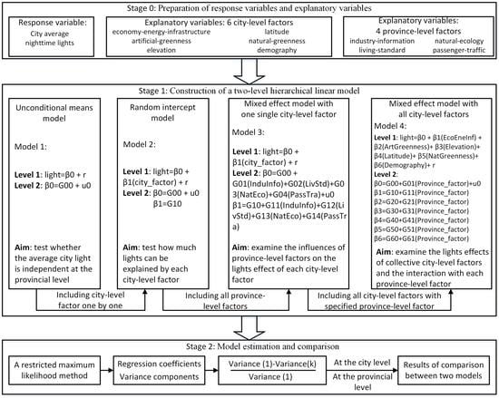
3.1. Construction of a Two-Level Hierarchical Linear Model
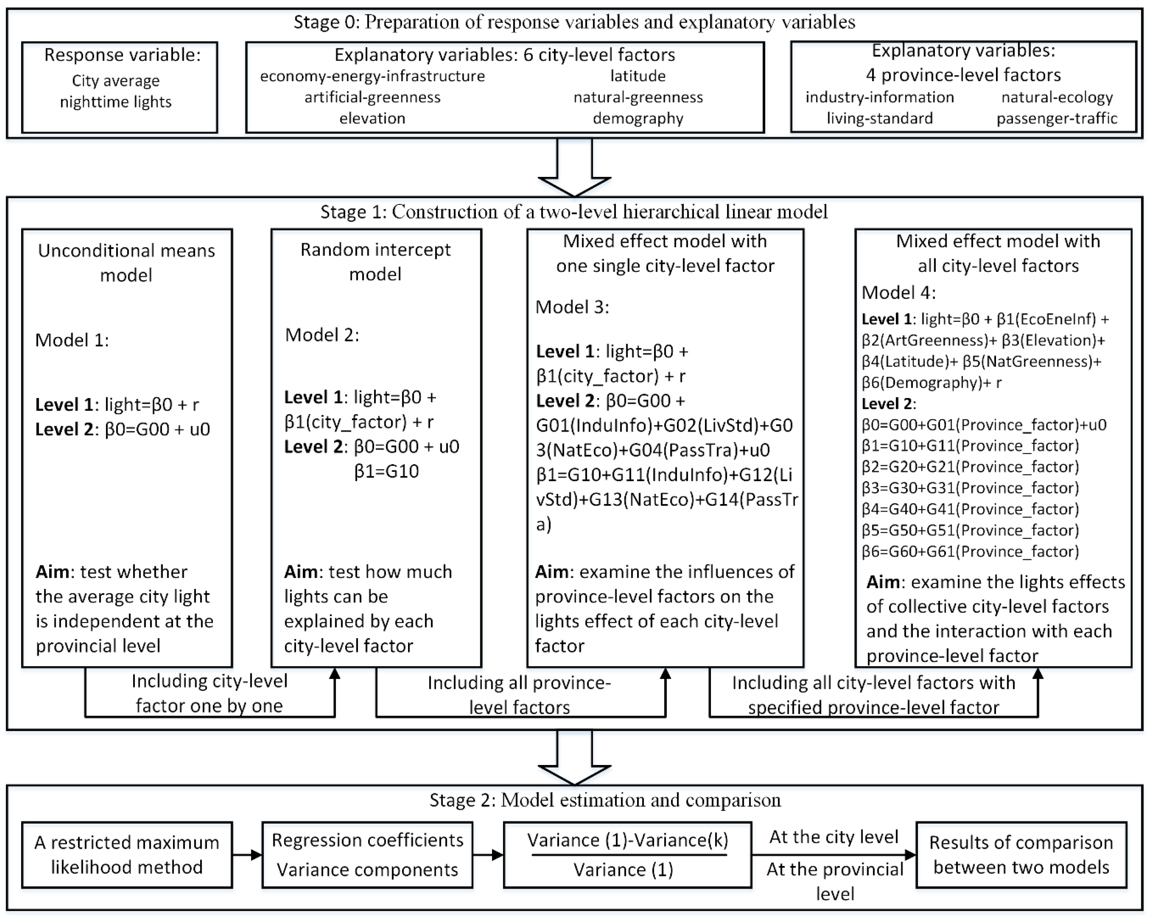
As shown in Figure 3, we developed a hierarchical linear model at the levels of city and province, including the unconditional means model, random intercept model, mixed-effect model with one single city-level factor, and mixed-effect model with all city-level factors.
3.1.1. Unconditional Means Model: Model 1
An unconditional means model is also known as the null model and was first developed to verify whether there are significant differences in nighttime lights in different provinces. As shown from Equation (1) to Equation (4), we present the two-level model and its variation components, where the response variable light of Equation (1) is the average nighttime light of a city, is the mean value of city light in a particular province, r is the random error of lights among cities, is the grand mean value of lights for all cities, is the random error of lights among provinces. It is assumed that the random error at the city or provincial level follows Gaussian normal distribution in terms of or . Thus, the variance of lights should be , and ICC denotes the intra-group correlation coefficient, which reflects the ratio of intra-group variance to the total variance. More specifically, if the average city light is independent at the provincial level, then there is no difference in nighttime lights in different provinces, which means the value of ICC is 0.
3.1.2. Random Intercept Model: Model 2
A random intercept model can be developed by introducing the city-level factor one by one to Model 1. In this respect, a total number of six sub-models of Model 2 are developed by adding the factors of economy-energy-infrastructure, artificial-greenness, elevation, latitude, natural-greenness, and demography, respectively. As shown in Equation (5) to Equation (7), we present the two-level model and the mixed model, where is the coefficient of the corresponding city-level factor.
3.1.3. Mixed-Effect Model with One Single City-Level Factor: Model 3
Based on Model 2, province-level factors are all added into the random intercept model at the provincial level, which is used to explain the slope and intercept at the city level. In this respect, a two-level mixed-effect model with one single city-level factor was developed, which led to six sub-models of Model 3 with respect to each city-level factor. As shown in Equation (8) to Equation (10), we display the corresponding two-level model and the mixed model, where , , , and represent the coefficients of province-level factors of industry-information, living-standard, natural-ecology, and passenger-traffic, respectively, and , , , and denote the coefficients of the interaction between each city-level factor and the four province-level factors, respectively. Specifically, the interactive coefficients can reflect the degrees of lights effects of a certain city-level factor and the corresponding interactions with the province-level factors.
3.1.4. Mixed-Effect Model with All City-Level Factors: Model 4
Based on Model 3, all city-level factors are added at the city level, but the four province-level factors are added one by one at the provincial level. In this respect, a two-level mixed-effect model with all city-level factors was developed, which led to four sub-models of Model 4 with respect to each province-level factor. It should be noted that this model was developed in a multivariate context and aimed to further improve the explaining capacity of factors at both the city level and provincial level. As shown in Equation (11) to Equation (13), we present the corresponding two-level model and the mixed model, where is coefficient of a particular province-level factor, , , , , , and represent the coefficients of city-level factors of economy-energy-infrastructure, artificial-greenness, elevation, latitude, natural-greenness, and demography, respectively, , , , , , and denote the coefficients of the interaction between each province-level factor and the six city-level factors, respectively. However, to avoid the complexity of the model, each province-level factor does not need to have interactions with all city-level factors. Instead, it has its own interactive pattern, as shown in Table 3. For instance, industry-information factor at the provincial level might affect the factors of economy-energy-infrastructure and demography at the city level, and thus the coefficients of and should be considered.
3.2. Model Estimation and Comparison
As shown in Figure 3, to estimate the regression coefficients and variance components of our hierarchical linear models, a restricted maximum likelihood method [36] was adopted, which is known as an efficient parameter estimator for multi-level models with normally distributed errors. This method can produce unbiased estimates of variance components and has been implemented in many popular statistical packages. In this study, we used the HLM 6.08 package for model estimation.
Once the variance components were estimated, we could compare two models in a quantitative way. Specifically, compared with Model 1, we can compute the percentage of variance explained by Model k at the city level and provincial level as and , respectively [29]. These are defined explicitly in Equation (14), where is the variance of lights difference in Model k at the city level, is the variance of lights difference in Model k at the provincial level, and k denotes the number of the model. In this respect, we could tell whether or how much one model is out-performed by the other one.
4. Analytic Results
4.1. Analysis of the Nighttime Lights Effects of Influencing Factors
4.1.1. Results of Unconditional Means Model: Model 1
As shown in Table 4, the value of ICC was calculated as 0.4990. Besides, the random variance u0 passed the chi-square test at a significance level of 1%, which meant that the value of ICC was statistically significant. Therefore, the results of Model 1 (null model) suggested that there were significant differences in nighttime lights across different provinces, and the province-level factors should not be ignored.
4.1.2. Results of Random Intercept Model: Model 2
As shown in Table 4, the following findings can be reported:
- 1)
- As for 2-1, there is a significant positive correlation between economy-energy-infrastructure factor and city lights. Specifically, with the increment of one unit of this factor, city lights might be increased by about 73.46% on average. This finding coincides well with many previous studies, which suggested that city lights are highly correlated with economic status [17], energy consumption [37], and urban infrastructure [38].
- 2)
- As for 2-2, the artificial-greenness factor is negatively correlated with city lights [38], but the influence is not significant. This is probably because green space in urban areas tends to be decorated with lighting facilities, which might affect the absorption and block of nighttime lights by vegetation. As for 2-3, elevation factor has a significant negative influence on city lights. Such situation coincides very well with the unbalanced development in Mainland China. In particular, cities in the northwest tend to be underdeveloped and are located at high altitudes, while those in the southwest are likely to be developed and are located at low altitudes. Specifically, with the increment of one unit of this factor, city lights might be decreased by about 11.69% on average.
- 3)
- As for 2-4 and 2-5, we can observe significant negative correlations between city lights and factors of latitude and natural-greenness. Such results are reasonable in the Chinese context because southern cities with low latitudes are more developed than northern cities with high latitudes, and cities with large coverages of vegetation tend to absorb or block more lights than those with small vegetation coverages [1]. Specifically, with one unit’s increase in latitude and natural-greenness, city lights could be decreased by 14.49% and 18.05%, respectively. However, as for 2-6, a significant positive correlation can be observed with the demography factor [22,39]. For instance, city lights might be increased by about 16.04% on average with the increment of one unit of this factor.
4.1.3. Results of the Mixed Effect Model with One Single City-Level Factor: Model 3
As shown in Table 5, the following findings could be observed:
- 1)
- In general, from model 3-1 to 3-6, we observed that the factors of industry-information, living-standard, and passenger-traffic at the provincial level had positive correlations with city lights, although some factors do not display significant influences. Moreover, the natural-ecology factor has a negative correlation with city lights, but it is not significant in most models. As indicated by the values of G10 in these models, each city-level factor had almost a similar influencing pattern as observed in Model 2, although the magnitude and significance of the effects varied slightly. For instance, artificial-greenness factor again showed a non-significant relationship with city lights, but the magnitude was relatively weak. These are probably due to the regulatory effects of province-level factors on each city-level factor [30].
- 2)
- Model 3-1 is a two-level mixed-effect model with economy-energy-infrastructure, and the results are shown in the second column of Table 5. Firstly, compared with the results of Model 2-1, the positive lights effect of economy-energy-infrastructure changes from 73.46% to 44.24% with a reduction of 39.78% on average, which further confirms the existence of intra-group and inter-group differences. Secondly, significant interactions can be observed for the lights effect of economy-energy-infrastructure with industry-information and passenger-traffic. Specifically, factors of industry-information and passenger-traffic can enhance the lights effects. For instance, a one-level increase in industry-information or passenger-traffic might significantly improve nighttime lights by 18.30% or 14.59% on average. The observed multiplying effect of economic activities from both provincial level and city level on lights indicates the important role of coordinated development of the regional economy. Thirdly, there are no significant interactions between the other two province-level factors and lights effects of economy-energy-infrastructure.
- 3)
- Model 3-2 is a two-level mixed-effect model with artificial-greenness, and the results are shown in the third column of Table 5. Firstly, compared with the results of Model 2-2, the non-significant negative lights effect of artificial-greenness is weakened by 66.67%, which is probably due to the regulatory effect of the natural-ecology factor at the provincial level. Secondly, natural-ecology factor has a significant interaction with the lights effect of artificial-greenness, which may have enhanced this negative influence. Specifically, with the increment of natural-ecology value in one unit, city lights will be decreased further by 4.07% on average. This is not surprising because forest area or natural conservation area in ecosystem can play a large role in cooling the cities [40]. Thirdly, the lights effect of artificial-greenness did not have significant interactions with other province-level factors, such as the factors of industry-information, living-standards, and passenger-traffic.
- 4)
- Model 3-3 is a two-level mixed-effect model with elevation, and the results are shown in the fourth column of Table 5. Firstly, the negative lights effect of elevation displays a slight decrease of 13.94% as compared with those of Model 2-3, and importantly, it becomes non-significant. This finding indicated that the impact of elevation on city lights might be unreliable by only considering their linear relationship. Secondly, there is a significant interaction between passenger-traffic factor and the lights effect of elevation, and passenger-traffic factor could reduce the negative effect of elevation. For instance, a one-level increase in passenger-traffic could significantly increase city lights by 1.84% on average. This finding is reasonable because urban transportation can improve urban economic development [41], which might lead to a high level of nighttime lights. Thirdly, there are no significant interactions between the lights effect of elevation and the factors of industry-information, living-standard, and natural-ecology.
- 5)
- The estimation results of Model 3-4 are summarized in the fifth column of Table 5. Firstly, compared with those of Model 2-4, the negative lights effect of latitude is diminished by a large percentage of 46.03% and becomes non-significant, which suggests that the impact of latitude on city lights might be unreliable by only considering their linear relationship. Secondly, the living-standard factor shows a significant interaction with the lights effect of latitude, which will continue to weaken this negative impact. For instance, with a one-level increase in living-standard, city lights will be increased largely by 26.81% on average. Thirdly, the natural-ecology factor displays a significant interaction with the lights effect of latitude, but the negative effect will be enhanced. For instance, city lights will be further decreased by 12.55% on average with the increment of one level’s natural-ecology factor. Fourthly, no significant interactions can be observed between city lights and the factors of industry-information and passenger-traffic.
- 6)
- The estimation results of Model 3-5 are shown in the sixth column of Table 5. First, it reports that the negative lights effect of natural-greenness is increased by a large percentage of 34.85% and remains significant. This finding implies the stability of the impact of natural-greenness on city lights for the entire Mainland China, which coincides well with a few previous studies [1,42]. Besides, this negative lights effect could be enhanced by a significant interaction with the natural-ecology factor, where city nights would be further decreased by 11.99% on average with one level’s increase on the value of natural-ecology factor. The finding can be given a similar explanation as elaborated in Model 3–2. Furthermore, the results suggest non-significant interactions between the lights effect of natural-greenness and the other three province-level factors.
- 7)
- The last column of Table 5 summarizes the estimation results of Model 3-6. Firstly, the positive lights effect of demography is increased by a large percentage of 49.84% and is still significant as compared with those of Model 2-6. This finding indicated the reliability of the relationship between city lights and demography, which agreed very well with those of most previous studies [22,39,43]. Secondly, the impact of demography on city lights is significant in its interactions with the factors of industry-information and living-standards. In particular, city lights will be further increased by 12.27% or 29.01% with the increment of one unit on industry-information or living-standard. This is reasonable because people are more likely to live in cities with more job opportunities and higher incomes [44]. Thirdly, there are no significant interactions between the lights effect of demography and the other two province-level factors.
4.1.4. Results of Mixed Effect Model with All City-Level Factors: Model 4
The estimation results from Model 4-1 to Model 4-4 are presented in Table 6. Collectively, economy-energy-infrastructure and demography had significant positive correlations with city lights, while elevation, latitude, and natural-greenness in most models were significantly negatively correlated with city lights. These results were roughly consistent with those of Model 3, although a major difference could be observed. For instance, artificial-greenness displayed a non-significant positive impact on city lights, which was different from the non-significant negative impact of Model 2 and Model 3. This finding reconfirmed the unreliability of artificial-greenness controlling city lights. Besides, factors of elevation and latitude become significant in most models as compared with those of Model 3, which implies that they might contribute lights collectively in a multivariate context.
In addition, industry-information can significantly enhance the lights effects of economy-energy-infrastructure and demography by further percentages of 19.92% and 0.72% in Model 4-1, which coincides well with those of Model 3-1 and 3-6. As for Model 4-2, living-standard can continue to significantly increase the positive lights effect of demography by around 26.74%, while its interaction with the positive lights effect of economy-energy-infrastructure is not significant. This finding also agrees well with those of Model 3-1 and 3-6. As for Model 4-3, natural-ecology had significant interactions with the lights effects of artificial-greenness and natural-greenness, which further imposed negative effects of 8.9% and 10.73%, respectively. However, its interactions with the negative lights effects of elevation and latitude were not significant, which roughly coincided with those of Model 3-2, 3-3, 3-4, and 3-5. Lastly, passenger-traffic displayed significant interactions with the lights effects of economy-energy-infrastructure and demography, which could enhance the positive effects of 15.98% and 10.71, respectively. Specifically, these interactions were much more significant than those of Model 3-1 and 3-6.
4.2. Model Comparisons and Variance Analysis
As shown in Table 7, the results can be summarized in the following points. (1) Compared with Model 1 (null model), the explained variances are all improved in Model 2 by adding city-level factors and in Model 3 by adding province-level factors. (2) The six sub-models of Model 3 can explain much more variances than the corresponding six sub-models of Model 2, which is mainly due to the significant interactive effects with the province-level factors. (3) The explained variances are dramatically improved in Model 4 with the percentages greater than 70% at the city level, which can be attributed mainly to the inclusion of all city-level factors; and they are higher than 90% at the provincial level, which is probably due to the interactive effects with the specified province-level factor. This further suggests the plausibility of Model 4. (4) The values of the -2LL (-2 multiplied by logarithmic likelihood) statistic decreased from Model 1 to Model 2 by adding each city-level factor, which indicated that Model 2 improved in terms of goodness-of-fit. (5) The inclusion of province-level factors led to a further reduction of the -2LL statistic value with respect to the six sub-models of Model 3, which hinted that each sub-model of Model 3 outperformed the corresponding sub-model of Model 2 in terms of goodness-of-fit. (6) Most of the -2LL statistic values in Model 4 further decreased compared to the ones in Model 3, which meant that Model 4 could give a better performance. (7) It should be noted that all the 17 models passed the KS (Kolmogorov–Smirnov) test at a significance level of 10%, which proved the effectiveness and superiority of our models.
5. Discussions and Limitations
Nevertheless, this study has a few issues worthy of discussion, which require further investigations.
Firstly, most of the correlations reported in this study can be substantiated and agree very well with the findings in the literature [1,17,22,37,38,39,42,43]. For instance, the negative lights effect of natural-greenness can be enhanced by a significant interaction with the natural-ecology factor at the provincial level, which implies the stability of the impact of natural-greenness on city lights for the entire Mainland China. However, the correlation with artificial-greenness becomes unstable and is not significant through our models, which might indicate that it was an unreliable factor controlling city lights. The reasons could be relevant to the decoration of lighting facilities, although we acknowledged the limitation of substantiating such a correlation. Besides, correlation with demography is positive and significant, but it does not mean that city lights can be a reliable estimator of population. On the one hand, city lights might function as a diverse number of factors in a multi-level manner. On the other hand, the increase in population does not necessarily lead to the expansion of urban areas, which follows that new public lighting installations might not be urgently needed [45]. In these respects, we attempted to substantiate our findings via comparisons with those in the literature. As for these new findings, we tried to give reasonable explanations, although they require further investigations.
Secondly, it is not an easy task to explain the differences in nighttime lights across different cities, because our analytic results can be affected by several issues, which might constitute potential limitations of our study. (1) New satellite products, such as Luojia-1 nighttime light imagery with high spatial resolution [46], can provide accurate estimates of nighttime lights, which might improve the statistical reliability of our results and require further studies. (2) Light emissions can vary differently with the zenith angle for different spectral bands [47], which means that light output patterns in different places can also be a potential issue affecting the differences in light emissions, and it needs further studies. (3) Light emissions could show seasonal behavior [1], which was neglected in our study owing to the usage of the annual average nighttime lights, and it poses a limitation. (4) Light emissions could be underestimated owing to the introduction of outdoor white LED lighting products because the VIIRS DNB sensor is not sensitive to the emission of blue light from LED sources. This is a common problem for the society of remote sensing of nighttime lights, but how it affects our results requires further studies. This relies on either the methodology to distinguish high-pressure sodium lamps from white LEDs or the design of new nighttime sensors with the ability to detect blue light. (5) Light emissions could be affected by the scattered lights near the city boundary, which were once thought to be an instrumental error but in fact represent a real detection of lights scattered in the atmosphere [48]. This problem appears to be obvious for brightly lit cities like Beijing and Shenzhen or urban agglomerations like the Yangtze River Delta Region, but it becomes trivial for most small- and medium-sized prefecture cities surrounded by rural areas. Considering its complicated characteristics, the extent to which it might affect our results needs further evaluations.
Thirdly, to some extent, our study could make some responses to the theory of regional development by validating the hypothesis that the inter-provincial variation contributes to the nighttime lights. For instance, industry-information, living-standard, and passenger-traffic present significant direct influences on the nighttime lights, being consistent with previous studies that indicated that regional socioeconomic factors could affect local nighttime lights. In terms of the interactive effects, industry-information and passenger-traffic at the provincial level can continue to enhance significantly the positive lights effect of economy-energy-infrastructure at the city level. Living-standard shows significant interaction with demography by strengthening its positive lights effect, and natural-ecology displays significant interactions with artificial-greenness and natural-greenness by increasing their negative light effects. These findings might agree well with the perspective of coordinated regional development, but it requires further studies to contribute to the theory of urban development by proposing a typology of nighttime lights of cities.
6. Conclusions
This study developed a two-level hierarchical linear model to explore nighttime lights effects of cross-level factors, which is different from conventional studies using regression models for a single level of factors. Based on our method, using the VIIRS nighttime light data in 2016, the experiment was conducted for 281 prefecture cities in Mainland China. Our results not only confirmed the findings of current studies on the correlation between city lights and socioeconomic factors, but it also reported significant correlations with other physical factors including elevation, passenger-traffic, natural-greenness, and others. Importantly, our results emphasized the underlying interactive lights effects of cross-level factors considering the hierarchical structure of anthropogenic development in space, which is traditionally neglected in the studies of factors controlling nighttime lights. In this respect, our study suggests that nighttime lights should be modeled and explained in a multi-level manner.
The findings of this study might benefit a better understanding of the mechanisms underlying nighttime light remote sensing and improve the reliability and effectiveness of relevant applications. (1) Variations of nighttime lights in space can be affected by a diverse number of factors organized in a hierarchical way, which means factors at a high level might impose a non-trivial impact on the nighttime lights through their interactions with the factors at a low level. (2) Because of the multi-level non-linear relationship between nighttime lights and a variety of factors, it should be very cautious to estimate some socioeconomic indicators using a simple regression of nighttime lights with only the measured socioeconomic values, such as GDP or population. (3) Nighttime light remote sensing has been widely applied to extract urban built-up areas and examine urban growth patterns. It should carefully use a specified threshold value to delineate the urban built-up area because lights brightness can be affected by many factors. For instance, the ambiguity of artificial-greenness might lead to unreliable estimation of threshold value.
Author Contributions
Conceptualization, T.J.; Data curation, K.C.; Formal analysis, T.J. and X.L.; Funding acquisition, T.J.; Methodology, T.J. and K.C.; Writing—original draft, T.J.; Writing—review & editing, T.J. and X.L. All authors have read and agreed to the published version of the manuscript.
Funding
This research was funded by the National Natural Science Foundation of China with grant number 41971332 and the APC was funded by the National Natural Science Foundation of China.
Acknowledgments
We thank the constructive comments from the editor and the anonymous reviewers.
Conflicts of Interest
The authors declare no conflict of interest.
References
- Levin, N.; Zhang, Q.L. A global analysis of factors controlling VIIRS nighttime light levels from densely populated areas. Remote Sens. Environ. 2017, 190, 366–382. [Google Scholar] [CrossRef] [Green Version]
- Jia, T.; Chen, K.; Wang, J. Characterizing the growth patterns of 45 major metropolitans in Mainland China using DMSP/OLS data. Remote Sens. 2017, 99, 571. [Google Scholar] [CrossRef] [Green Version]
- Elvidge, C.D.; Baugh, K.E.; Kihn, E.A.; Kroehl, H.W.; Davis, E.R. Mapping of city lights using DMSP Operational Linescan System data. Photogramm. Eng. Remote Sens. 1997, 63, 727–734. [Google Scholar]
- Levin, N.; Kyba, C.; Zhang, Q.; De Miguel, A.S.; Roman, M.O.; Li, X.; Portnov, B.A.; Molthan, A.L.; Jechow, A.; Miller, S.D.; et al. Remote sensing of night lights: A review and an outlook for the future. Remote Sens. Environ. 2020, 237, 111443. [Google Scholar] [CrossRef]
- Small, C.; Elvidge, C.D. Night on Earth: Mapping decadal changes of anthropogenic night light in Asia. Int. J. Appl. Earth Obs. Geoinf. 2013, 22, 40–52. [Google Scholar] [CrossRef] [Green Version]
- Small, C.; Pozzi, F.; Elvidge, C.D. Spatial analysis of global urban extent from DMSPOLS night lights. Remote Sens. Environ. 2005, 96, 277–291. [Google Scholar] [CrossRef]
- Li, X.; Elvidge, C.D.; Zhou, Y.; Cao, C.; Warner, T. Remote sensing of night-time light. Int. J. Remote Sens. 2017, 3838, 5855–5859. [Google Scholar] [CrossRef] [Green Version]
- Shi, K.F.; Yu, B.L.; Huang, Y.X.; Hu, Y.J.; Yin, B.; Chen, Z.Q.; Chen, L.J.; Wu, J.P. Evaluating the Ability of NPP-VIIRS Nighttime Light Data to Estimate the Gross Domestic Product and the Electric Power Consumption of China at Multiple Scales: A Comparison with DMSP-OLS Data. Remote Sens. 2014, 6, 1705–1724. [Google Scholar] [CrossRef] [Green Version]
- Ou, J.; Liu, X.; Li, X.; Li, M.; Li, W. Evaluation of NPP-VIIRS Nighttime Light Data for Mapping Global Fossil Fuel Combustion CO2 Emissions: A Comparison with DMSP-OLS Nighttime Light Data. PLoS ONE 2015, 10, e138310. [Google Scholar]
- Ghosh, T.; Anderson, S.; Elvidge, C.D.; Sutton, P.C. Using nighttime satellite imagery as a proxy measure of human well-being. Sustainability 2013, 5, 4988–5019. [Google Scholar] [CrossRef] [Green Version]
- Chen, X.; Nordhaus, W.D. Using luminosity data as a proxy for economic statistics. Proc. Natl. Acad. Sci. USA 2011, 108, 8589–8594. [Google Scholar] [CrossRef] [PubMed] [Green Version]
- Ma, T.; Zhou, C.; Pei, T.; Haynie, S.; Fan, J. Responses of Suomi-NPP VIIRS-derived nighttime lights to socioeconomic activity in China’s cities. Remote Sens. Lett. 2014, 5, 165–174. [Google Scholar] [CrossRef]
- Kyba, C.C.M.; Garz, S.; Kuechly, H.; Miguel, A.S.; Zamorano, J.; Fischer, J.; Hölker, F. High-Resolution Imagery of Earth at Night: New Sources, Opportunities and Challenges. Remote Sens. 2014, 7, 1–23. [Google Scholar] [CrossRef] [Green Version]
- Zhao, M.; Cheng, W.; Zhou, C.; Li, M.; Wang, N.; Liu, Q. GDP spatialization and economic differences in South China based on NPP-VIIRS nighttime light imagery. Remote Sens. 2017, 9, 673. [Google Scholar] [CrossRef] [Green Version]
- Ma, T. Multi-Level Relationships between Satellite-Derived Nighttime Lighting Signals and Social Media-Derived Human Population Dynamics. Remote Sens. 2018, 10, 1128. [Google Scholar] [CrossRef] [Green Version]
- Sun, Y.W.; Gao, C.; Li, J.L.; Li, W.F.; Ma, R.F. Examining urban thermal environment dynamics and relations to biophysical composition and configuration and socio-economic factors: A case study of the Shanghai metropolitan region. Sustain. Cities Soc. 2018, 40, 284–295. [Google Scholar] [CrossRef]
- Chen, X.; Nordhaus, W.D. VIIRS Nighttime Lights in the Estimation of Cross-Sectional and Time-Series GDP. Remote Sens. 2019, 11, 1057. [Google Scholar] [CrossRef] [Green Version]
- Li, S.Y.; Cheng, L.; Liu, X.Q.; Mao, J.Y.; Wu, J.; Li, M.C. City type-oriented modeling electric power consumption in China using NPP-VIIRS nighttime stable light data. Energy 2019, 189, 116040. [Google Scholar] [CrossRef]
- Guk, E.; Levin, N. Analyzing spatial variability in night-time lights using a high spatial resolution color Jilin-1 image—Jerusalem as a case study. ISPRS J. Photogramm. Remote Sens. 2020, 163, 121–136. [Google Scholar] [CrossRef]
- Zhao, N.Z.; Cao, G.F.; Zhang, W.; Samson, E.L.; Chen, Y. Remote sensing and social sensing for socioeconomic systems: A comparison study between nighttime lights and location-based social media at the 500 m spatial resolution. Int. J. Appl. Earth Obs. Geoinf. 2020, 87, 102058. [Google Scholar] [CrossRef]
- Ma, T.; Zhou, Y.; Wang, Y.; Zhou, C.; Haynie, S.; Xu, T. Diverse relationships between Suomi-NPP VIIRS night-time light and multi-scale socioeconomic activity. Remote Sens. Lett. 2014, 5, 652–661. [Google Scholar] [CrossRef]
- Hu, Y.; Zhao, G.; Zhang, Q.L. Spatial Distribution of Population Data Based on Nighttime Light and LUC Data in the Sichuan Chongqing Region. J. Geoinf. Sci. 2018, 20, 68–78. [Google Scholar]
- Fu, D.; Xia, X.; Duan, M.; Zhang, X.; Li, X.; Wang, J.; Liu, J. Mapping nighttime PM2.5 from VIIRS DNB using a linear mixed-effect model. Atmos. Environ. 2018, 178, 214–222. [Google Scholar] [CrossRef]
- Zhu, X.; Ma, M.; Yang, H.; Ge, W. Modeling the spatiotemporal dynamics of gross domestic product in China using extended temporal coverage nighttime light data. Remote Sens. 2017, 9, 626. [Google Scholar] [CrossRef] [Green Version]
- Zhao, M.; Zhou, Y.; Li, X.; Cao, W.; He, C.; Yu, B.; Li, X.; Elvidge, C.D.; Cheng, W.; Zhou, C. Applications of satellite remote sensing of nighttime light observation: Advances, challenges, and perspectives. Remote Sens. 2019, 11, 1971. [Google Scholar] [CrossRef] [Green Version]
- Jia, T.; Yu, X.; Shi, W.; Liu, X.; Li, X.; Xu, Y. Detecting the regional delineation from a network of social media user interaction with spatial constraint: A case study of Shenzhen, China. Phys. A: Stat. Mech. Appl. 2019, 531, 121719. [Google Scholar] [CrossRef]
- Du, Q.; Yu, H. Multidimensional urban spatial structure and regional income disparity. Sci. Geogr. Sin. 2020, 40, 720–729. [Google Scholar]
- Diez-Roux, A.V. Bringing context back into epidemiology: Variables and fallacies in multilevel analysis. Am. J. Public Health 1998, 88, 216–222. [Google Scholar] [CrossRef] [Green Version]
- Raudenbush, S.W.; Bryk, A.S. Hierarchical Linear Models: Applications and Data Analysis Methods, 2nd ed.; SAGE Publications: Thousand Oaks, CA, USA, 2002. [Google Scholar]
- Zhang, Y.; Jin, Y.; Zhu, T. The health effects of individual characteristics and environmental factors in China: Evidence from the hierarchical linear model. J. Clean. Prod. 2018, 194, 554–563. [Google Scholar] [CrossRef]
- Keng, C.W.K. China’s Unbalanced Economic Growth. J. Contemp. China 2006, 15, 183–214. [Google Scholar] [CrossRef]
- Li, H.; Wei, Y.; Liao, F.H.; Huang, Z. Administrative hierarchy and urban land expansion in transitional China. Appl. Geogr. 2015, 56, 177–186. [Google Scholar] [CrossRef]
- Clinton, N.; Yu, L.; Gong, P. Geographic stacking: Decision fusion to increase global land cover map accuracy. ISPRS J. Photogramm. Remote Sens. 2015, 103, 57–65. [Google Scholar] [CrossRef]
- Jia, T.; Li, Y.; Shi, W.; Zhu, L. Deriving a Forest Cover Map in Kyrgyzstan Using a Hybrid Fusion Strategy. Remote Sens. 2019, 11, 2325. [Google Scholar] [CrossRef] [Green Version]
- Tian, J.; Zhao, N.; Samson, E.; Wang, S. Brightness of Nighttime Lights as a Proxy for Freight Traffic: A Case Study of China. Brightness of Nighttime Lights as a Proxy for Freight Traffic: A Case Study of China. IEEE J. Sel. Top. Appl. Earth Obs. Remote Sens. 2014, 7, 206–212. [Google Scholar] [CrossRef]
- Boedeker, P. Hierarchical Linear Modeling with Maximum Likelihood, Restricted Maximum Likelihood, and Fully Bayesian Estimation. Pract. Assess. Res. Eval. 2017, 22, 1–19. [Google Scholar]
- Lin, J.; Shi, W. Statistical correlation between monthly electric power consumption and VIIRS Nighttime Light. ISPRS Int. J. Geo-Inf. 2020, 9, 32. [Google Scholar] [CrossRef] [Green Version]
- Dou, Y.; Liu, Z.; He, C.; Yue, H. Urban Land Extraction Using VIIRS Nighttime Light Data: An Evaluation of Three Popular Methods. Remote Sens. 2017, 9, 175. [Google Scholar] [CrossRef] [Green Version]
- Tan, M.; Li, X.; Li, S.; Xin, L.; Wang, X.; Li, Q.; Li, W.; Li, Y.; Xiang, W. Modeling population density based on nighttime light images and land use data in China. Appl. Geogr. 2018, 90, 239–247. [Google Scholar] [CrossRef]
- Lane, K.J.; Stokes, E.C.; Seto, K.C.; Thanikachalam, S.; Thanikachalam, M.; Bell, M.L. Associations between Greenness, Impervious Surface Area, and Nighttime Lights on Biomarkers of Vascular Aging in Chennai, India. Environ. Health Perspect. 2017, 125, 087003. [Google Scholar] [CrossRef] [PubMed] [Green Version]
- Mayer, T.; Trevien, C. The impact of urban public transportation evidence from the Paris region. J. Urban Econ. 2017, 102, 1–21. [Google Scholar] [CrossRef] [Green Version]
- Levin, N. The impact of seasonal changes on observed nighttime brightness from 2014 to 2015 monthly VIIRS DNB composites. Remote Sens. Environ. 2017, 193, 150–164. [Google Scholar] [CrossRef]
- Chu, H.J.; Yang, C.H.; Chou, C.C. Adaptive Non-Negative Geographically Weighted Regression for Population Density Estimation Based on Nighttime Light. ISPRS Int. J. Geo-Inf. 2019, 8, 26. [Google Scholar] [CrossRef] [Green Version]
- Ranganathan, S.; Swain, R.; Sumpter, D. The demographic transition and economic growth: Implications for development policy. Palgrave Commun. 2015, 1, 15033. [Google Scholar] [CrossRef] [Green Version]
- Kocifaj, M.; Komar, L.; Lamphar, H.; Wallner, S. Are population-based models advantageous in estimating the lumen outputs from light-pollution sources? Mon. Not. R. Astron. Soc. Lett. 2020, 496, L138–L141. [Google Scholar] [CrossRef]
- Li, X.; Li, X.Y.; Li, D.; He, X.; Jendryke, M. A preliminary investigation of Luojia-1 night-time light imagery. Remote Sens. Lett. 2019, 10, 526–535. [Google Scholar] [CrossRef]
- Kocifaj, M.; Solano-Lamphar, H.A.; Videen, G. Night-sky radiometry can revolutionize the characterization of light-pollution sources globally. Proc. Natl. Acad. Sci. USA 2019, 116, 7712–7717. [Google Scholar] [CrossRef] [Green Version]
- De Miguel, A.S.; Kyba, C.; Zamorano, J.; Gallego, J.; Gaston, K.J. The nature of the diffuse light near cities detected in nighttime satellite imagery. Sci. Rep. 2020, 10, 1–16. [Google Scholar]
Figure 1.
The selected 281 prefecture cities in Mainland China (Note: they are unevenly separated by the Aihui-Tengchong Line, which indicates the unbalanced distribution of the population).
Figure 1.
The selected 281 prefecture cities in Mainland China (Note: they are unevenly separated by the Aihui-Tengchong Line, which indicates the unbalanced distribution of the population).

Figure 2.
The geographical datasets: (a) VIIRS DNB nighttime annual stable lights in 2016; (b) MODIS NDVI product in 2016; and (c) Digital Elevation Model (DEM) dataset in 2016.
Figure 2.
The geographical datasets: (a) VIIRS DNB nighttime annual stable lights in 2016; (b) MODIS NDVI product in 2016; and (c) Digital Elevation Model (DEM) dataset in 2016.


Figure 3.
A flowchart for exploring the factors controlling nighttime lights with a hierarchical linear model.
Figure 3.
A flowchart for exploring the factors controlling nighttime lights with a hierarchical linear model.


Table 1.
Selection of variables at the city level and provincial level.
| 12 Variables at the City Level | 16 Variables at the Provincial Level | ||
|---|---|---|---|
| GDP | An economic variable | Primary industrial added value | An industrial variable |
| GDP per capita | An economic variable | Secondary industrial added value | An industrial variable |
| Population | A demographic variable | Tertiary industrial added value | An industrial variable |
| Population density | A demographic variable | Total sales of consumer goods | An economic variable |
| Total electric consumption | An energy-related variable | Total amount of fixed assets investment | An economic variable |
| Road area | An infrastructure-related variable | Number of mobile phone users | An ICT-related variable |
| Number of internet users | An ICT-related variable | ||
| Urban built-up area | An infrastructure-related variable | Number of broadband access users | An ICT-related variable |
| Total passenger traffic | A transport-related variable | ||
| Personal city green space area | An urban ecological variable | Road passenger traffic | A transport-related variable |
| Rail passenger traffic | A transport-related variable | ||
| Personal urban green coverage area | An urban ecological variable | Personal wages | A living standard variable |
| Personal disposable income | A living standard variable | ||
| Average NDVI | A natural ecological variable | Personal consumption expenditure | A living standard variable |
| Average elevation | A geographical variable | Forest area | A natural ecological variable |
| Latitude | A geographical variable | Natural ecological conservation area | A natural ecological variable |
Table 2.
Derivation of factors at the city level and provincial level using PCA analysis. Note: percentages in bold indicate the proportion of total variance that can be explained by the selected factors.
Table 2.
Derivation of factors at the city level and provincial level using PCA analysis. Note: percentages in bold indicate the proportion of total variance that can be explained by the selected factors.
| 6 Factors at the City Level | 4 Factors at the Provincial Level | ||||||
|---|---|---|---|---|---|---|---|
| Factors | Eigenvalues | Percentage | Cumulative | Factors | Eigenvalues | Percentage | Cumulative |
| economy-energy-infrastructure | 5.02 | 41.80% | 41.80% | industry-information | 9.34 | 58.39% | 58.39% |
| artificial-greenness | 1.81 | 15.06% | 56.86% | living-standard | 3.52 | 22.00% | 80.39% |
| elevation | 1.27 | 10.54% | 67.40% | natural-ecology | 1.09 | 6.82% | 87.21% |
| latitude | 0.96 | 8.04% | 75.44% | ||||
| natural-greenness | 0.92 | 7.63% | 83.07% | passenger-traffic | 0.78 | 4.88% | 92.09% |
| demography | 0.70 | 5.85% | 88.92% | ||||
Table 3.
Coefficients of explanatory factors in Model 4.
| Industry-Information | Living-Standard | Natural-Ecology | Passenger-Traffic | |
|---|---|---|---|---|
| Model | Model 4-1 | Model 4-2 | Model 4-3 | Model 4-4 |
| economy-energy-infrastructure | ||||
| artificial-greenness | ||||
| elevation | ||||
| latitude | ||||
| natural-greenness | ||||
| demography | ||||
| economy-energy-infrastructure | —— | |||
| artificial-greenness | —— | —— | —— | |
| elevation | —— | —— | —— | |
| latitude | —— | —— | —— | |
| natural-greenness | —— | —— | —— | |
| demography | —— |
Table 4.
The estimation of parameters and variance components (with standard errors) for Model 1 and Model 2 (Note: *, **, and *** denote the significance level at 10%, 5%, and 1%, respectively).
Table 4.
The estimation of parameters and variance components (with standard errors) for Model 1 and Model 2 (Note: *, **, and *** denote the significance level at 10%, 5%, and 1%, respectively).
| Model | 1 | 2-1 | 2-2 | 2-3 | 2-4 | 2-5 | 2-6 |
|---|---|---|---|---|---|---|---|
| Fixed effect: | |||||||
| G00 | 0.1398 (0.1643) | −0.1096 (0.1456) | 0.1716 (0.1901) | 0.1942 * (0.1754) | 0.1698 * (0.1777) | 0.1729 * (0.1753) | 0.1440 (0.1747) |
| G10 | —— | 0.7346 *** (0.0450) | −0.1791 (0.1704) | −0.1169 * (0.0780) | −0.1449 * (0.0852) | −0.1805 ** (0.0498) | 0.1604 *** (0.0542) |
| Variance components: | |||||||
| σ2 | 0.6974 (0.8351) | 0.3447 (0.5872) | 0.6509 (0.8068) | 0.6882 (0.8296) | 0.6799 (0.8246) | 0.6767 (0.8226) | 0.6729 (0.8203) |
| τ00 | 0.6947 *** (0.8335) | —— | —— | —— | —— | —— | —— |
Table 5.
The estimation of parameters and variance components (with standard errors) for Model 3 (Note: *, **, and *** denote the significance level at 10%, 5%, and 1%, respectively).
Table 5.
The estimation of parameters and variance components (with standard errors) for Model 3 (Note: *, **, and *** denote the significance level at 10%, 5%, and 1%, respectively).
| Model | 3-1 (Economy-Energy-Infrastructure) | 3-2 (Artificial-Greenness) | 3-3 (Elevation) | 3-4 (Latitude) | 3-5 (Natural-Greenness) | 3-6 (Demography) |
|---|---|---|---|---|---|---|
| Fixed effect: | ||||||
| G00 | 0.0210 (0.0514) | −0.2613 (0.1069) | 0.1057 (0.1102) | 0.1652 * (0.0929) | 0.2666 ** (0.1310) | 0.2127 *** (0.0904) |
| G01 | 0.0735 * (0.0384) | 0.1375 *** (0.0840) | 0.1340 * (0.0595) | 0.1322 * (0.0645) | 0.1321 (0.0796) | 0.2221 *** (0.0580) |
| G02 | 0.3366 ** (0.0655) | 0.9793 ** (0.2353) | 0.7337 *** (0.2075) | 0.7643 ** (0.2266) | 1.0553 *** (0.3045) | 0.9073 ** (0.1856) |
| G03 | −0.0071 (0.0341) | −0.0258 (0.0652) | −0.0597 * (0.0520) | −0.0769 (0.0480) | −0.0213* (0.0620) | −0.0084 (0.0342) |
| G04 | 0.0166 (0.0474) | 0.0429 (0.0793) | 0.0152 (0.0552) | 0.0034 *** (0.0681) | 0.0067 (0.0573) | 0.0166 (0.0569) |
| G10 | 0.4424 *** (0.0789) | −0.0597 (0.1087) | −0.1006 (0.0781) | −0.0782 (0.1078) | −0.2343 *** (0.1085) | 0.2405 ** (0.0940) |
| G11 | 0.1830 * (0.0497) | 0.2385 (0.0620) | 0.0937 (0.0872) | 0.0620 (0.0804) | 0.0041 (0.0765) | 0.1227 *** (0.0379) |
| G12 | 0.0535 (0.0568) | 0.0664 (0.2468) | 0.1151 (0.1255) | 0.2681 * (0.2103) | 0.2651 (0.1347) | 0.2901 * (0.1746) |
| G13 | −0.1449 (0.0661) | −0.0407 * (0.0328) | −0.0236 (0.0512) | −0.1255 * (0.0472) | −0.1199 * (0.0709) | −0.0150 (0.0319) |
| G14 | 0.1459 * (0.1070) | 0.1316 (0.1195) | 0.0184 * (0.0748) | 0.0631 (0.0796) | 0.0092 (0.0388) | 0.0674 (0.0355) |
| Variance components: | ||||||
| σ2 | 0.3199 (0.5655) | 0.5963 (0.7458) | 0.6484 (0.8417) | 0.6366 (0.8346) | 0.6247 (0.8152) | 0.6017 (0.8134) |
| τ00 | 0.0190 *** (0.1379) | 0.1173 *** (0.3425) | 0.1247 *** (0.3605) | 0.1242 *** (0.3578) | 0.1904 *** (0.4017) | 0.1217 *** (0.3521) |
Table 6.
The estimation of parameters and variance components (with standard errors) for Model 4 (Note: *, **, and *** denote the significant level at 10%, 5%, and 1%, respectively).
Table 6.
The estimation of parameters and variance components (with standard errors) for Model 4 (Note: *, **, and *** denote the significant level at 10%, 5%, and 1%, respectively).
| Model | 4-1 (Industry-Information) | 4-2 (Living-Standard) | 4-3 (Natural-Ecology) | 4-4 (Passenger-Traffic) | |||
|---|---|---|---|---|---|---|---|
| Fixed effect: | |||||||
| G00 | −0.0734 (0.0950) | 0.1236 *** (0.0969) | 0.0025 (0.0791) | −0.0063 (0.0647) | |||
| G10 | 0.5605 *** (0.1108) | 0.6237 *** (0.1530) | 0.7136 *** (0.1320) | 0.7564 *** (0.1225) | |||
| G20 | 0.0345 (0.0668) | 0.0728 (0.0970) | 0.0733 (0.0960) | 0.0697 (0.0902) | |||
| G30 | −0.1205 ** (0.0646) | −0.2056 * (0.0750) | −0.1569 * (0.0785) | −0.1503 *** (0.0709) | |||
| G40 | −0.0321 (0.0582) | −0.0318 * (0.0563) | −0.0150 (0.0606) | −0.0693 ** (0.0555) | |||
| G50 | −0.1036 * (0.0739) | −0.0948 ** (0.0725) | −0.0790 * (0.0763) | −0.1346 ** (0.0650) | |||
| G60 | 0.0356 * (0.0337) | 0.1591 *** (0.0554) | 0.0460 * (0.0635) | 0.0387 * (0.0284) | |||
| G01 | 0.0394 (0.0546) | 0.3288 ** (0.2326) | −0.0653 (0.0795) | 0.0681 ** (0.0525) | |||
| G11 | 0.1992 *** (0.0533) | 0.0231 (0.0641) | —— | 0.1598 * (0.1084) | |||
| G21 | —— | —— | −0.0890 * (0.0551) | —— | |||
| G31 | —— | —— | −0.0049 (0.0705) | —— | |||
| G41 | —— | —— | −0.0372 (0.0891) | —— | |||
| G51 | —— | —— | −0.1073 ** (0.0727) | —— | |||
| G61 | 0.0072 ** (0.0479) | 0.2674 ** (0.1261) | —— | 0.1071* (0.0488) | |||
| Variance components: | |||||||
| σ2 | 0.1578 (0.5306) | 0.1670 (0.5398) | 0.1783 (0.5402) | 0.1876 (0.5521) | |||
| τ00 | 0.0477 *** (0.5988) | 0.0485 *** (0.6012) | 0.0595 *** (0.6215) | 0.0618 *** (0.6411) | |||
Table 7.
Variance explained by the models and their statistical tests.
| Model | PVEcity | PVEprovince | -2LL stat. | KS stat. |
|---|---|---|---|---|
| 1. | —— | —— | 760.04 | 0.287(0.000) |
| 2-1 | 50.56% | —— | 575.94 | 0.215(0.000) |
| 2-2 | 6.66% | —— | 752.04 | 0.173(0.000) |
| 2-3 | 1.31% | —— | 759.26 | 0.082(0.000) |
| 2-4 | 2.51% | —— | 758.90 | 0.049(0.099) |
| 2-5 | 2.96% | —— | 756.20 | 0.079(0.000) |
| 2-6 | 3.51% | —— | 755.82 | 0.091(0.000) |
| 3-1 | 54.13% | 97.26% | 522.20 | 0.163(0.000) |
| 3-2 | 14.49% | 83.11% | 685.44 | 0.209(0.000) |
| 3-3 | 7.01% | 82.06% | 727.94 | 0.200(0.000) |
| 3-4 | 8.71% | 82.12% | 726.26 | 0.279(0.000) |
| 3-5 | 10.42% | 72.60% | 725.08 | 0.235(0.000) |
| 3-6 | 13.72% | 82.48% | 715.46 | 0.186(0.000) |
| 4-1 | 77.37% | 93.14% | 538.28 | 0.137(0.000) |
| 4-2 | 76.06% | 93.01% | 555.58 | 0.130(0.000) |
| 4-3 | 74.43% | 91.44% | 585.58 | 0.147(0.000) |
| 4-4 | 73.09% | 91.11% | 564.08 | 0.142(0.000) |
© 2020 by the authors. Licensee MDPI, Basel, Switzerland. This article is an open access article distributed under the terms and conditions of the Creative Commons Attribution (CC BY) license (http://creativecommons.org/licenses/by/4.0/).
Share and Cite
MDPI and ACS Style
Jia, T.; Chen, K.; Li, X. Exploring the Factors Controlling Nighttime Lights from Prefecture Cities in Mainland China with the Hierarchical Linear Model. Remote Sens. 2020, 12, 2119. https://doi.org/10.3390/rs12132119
AMA Style
Jia T, Chen K, Li X. Exploring the Factors Controlling Nighttime Lights from Prefecture Cities in Mainland China with the Hierarchical Linear Model. Remote Sensing. 2020; 12(13):2119. https://doi.org/10.3390/rs12132119
Chicago/Turabian StyleJia, Tao, Kai Chen, and Xin Li. 2020. "Exploring the Factors Controlling Nighttime Lights from Prefecture Cities in Mainland China with the Hierarchical Linear Model" Remote Sensing 12, no. 13: 2119. https://doi.org/10.3390/rs12132119
Note that from the first issue of 2016, this journal uses article numbers instead of page numbers. See further details here.