Identification of Poverty Areas by Remote Sensing and Machine Learning: A Case Study in Guizhou, Southwest China


1
Center for China Western Modernization, Guizhou University of Finance and Economics, University City, Huaxi District, Guiyang 550025, China
2
College of Big Data Application and Economic, Guizhou University of Finance and Economics, University City, Huaxi District, Guiyang 550025, China
*
Author to whom correspondence should be addressed.
ISPRS Int. J. Geo-Inf. 2021, 10(1), 11; https://doi.org/10.3390/ijgi10010011
Submission received: 11 November 2020
/
Revised: 21 December 2020
/
Accepted: 27 December 2020
/
Published: 30 December 2020
(This article belongs to the Special Issue Geo-Information Technology and Its Applications)
Abstract
:As an objective social phenomenon, poverty has accompanied the vicissitudes of human society, which is a chronic dilemma hindering human civilization. Remote sensing data, such as nighttime lights imagery, provides abundant poverty-related information that can be related to poverty. However, it may be insufficient to rely merely on nighttime lights data, because poverty is a comprehensive problem, and poverty identification may be affected by topography, especially in some developing countries or regions where agriculture accounts for a large proportion. Therefore, some geographical features may be necessary for supplements. With the support of the random forest machine learning method, we extracted 23 spatial features base on remote sensing including nighttime lights data and geographical data, and carried out the poverty identification in Guizhou Province, China, since 2012. Compared with the identifications using support vector machines and the artificial neural network, random forest showed a better accuracy. The results supported that nighttime lights and geographical features are better than those only by nighttime lights features. From 2012 to 2019, the identified poor counties in Guizhou Province showed obvious dynamic spatiotemporal characteristics. The number of poor counties has decreased consistently and contiguous poverty-stricken areas have fragmented; the number of poor counties in the northeast and southwest regions decreased faster than other areas. The reduction in poverty probability exhibited a pattern of spreading from the central and northern regions to the periphery parts. The poverty reduction was relatively slow in areas with large slope and large topographic relief. When poor counties are adjacent to more non-poor counties, they can get rid of poverty easier. This study provides a method for feature selection and recognition of poor counties by remote sensing images and offers new insights into poverty identification and regional sustainable development for other developing countries and areas.
1. Introduction
As an objective social phenomenon, poverty has accompanied the vicissitudes of human society, which is a chronic dilemma hindering human civilization [1]. China, the world’s largest developing country, has been undergoing rapid economic development [2]. In the past years, China has taken a large number of comprehensive poverty-alleviation work and has achieved remarkable success in poverty reduction since the beginning of the economic reforms [3]. China was therefore the first country in the world to successfully achieve the target of Millennium Development Goals of having extreme poverty in 2012, which was ahead of schedule [4]. However, there are still a large number of poor people, and, at the same time, new aspects of poverty have emerged in China. Poverty remains a serious issue for China’s modernization [5]. In Southwest China, the high altitude and mountainous terrain lead to the low efficiency of land use and the underdeveloped transportation, which are the important causes of poverty [6]. Guizhou, a relatively poor province in Southwest China, has more mountainous areas, less flat land, and backward economic development [7]. Coordinating regional development, reducing poverty, and preventing the reoccurrence of poverty are the major challenges of its social and economic development [8].
Being able to accurately identify poor areas is the underlying premise of poverty reduction [8]. The spatiotemporal analysis of poverty is conducive to the formulation of regional policies for the purpose of poverty-alleviation [9]. Traditionally, the data sources for poverty assessment are the census or household surveys collected by local governments or national organizations [10,11]. Although the quality and quantity of economic data for developing countries have improved recently, a lack of data remains a major obstacle for relevant assessment [12]. In particular, the data related to poverty are usually scarce and inadequate in coverage. As the poverty research involves multi-dimensional assessment currently, more accurate indicators are needed to support poverty identification [13]. The substantial monetary cost, time and effort required to perform a census or survey means that developing countries can only conduct them periodically [14]. Moreover, different calibers of data sources make it extremely difficult to have a dynamic spatiotemporal analysis of poverty [9]. In addition, not all countries or organizations conduct periodical in-depth surveys [15]. The limitations of traditional data sources have posed great challenges to the identification of regional poverty in developing countries and areas [9].
Compared to traditional data, remote sensing data are unique, objective, consistent, and valuable resources that can provide spatial information for a variety of research purposes [16]. However, remote sensing cannot completely replace the traditional poverty identification. For example, the survey of household income and subjective feelings of poverty cannot be obtained by remote sensing. However, remote sensing technology has certain advantages in the spatial identification of poverty, which can reduce the workload of surveys and statistics [11]. Many scholars have demonstrated that poverty can be investigated using remote sensing [9,11,13,17,18,19,20,21,22,23,24]. The research areas mainly include regional poverty identification [8,9], slum mapping [17,18,19,20,21,22], and the link of the morphological structure to social poverty [23,24,25]. The first one is mainly used to solve the problem of identifying contiguous poverty areas at a large scale [9]. The latter two have advantages in solving slums investigation and urban problems [19,20,21], mostly based on high-resolution remote sensing data [23,24]. Rural poverty is the main form of poverty in China [26]. According to the government survey, by the end of 2018, there were 16.60 million rural poor people in China, most of whom lived in mountainous areas [27,28]. The poor counties are usually obviously contiguous in space, while the farmers’ houses are scattered in vast rural areas [29]. The high-spatial-resolution recognition of poor residential areas is affected by the complexity of underlying surface [17]. Using morphological structure recognition or slum mapping to study this kind of regional poverty problem has certain challenges.
Nighttime light imagery, which is a common remote sensing data source, has been successfully used to explore changes in human activities. As one of the few reproducible and objective observation sources on a global scale, it has been used for research on regional issues including ecological civilization, social economy, urbanization, and energy-related issues, with a great reduction of statistical costs [30,31,32]. Recently, there have been promising signs that nighttime light imagery can provide accurate and up-to-date indications of regional poverty [11,13,15,33,34,35]. However, mostly studies used imagery in combination with statistical data [36]; thus, they were restricted by the statistical data. The advantages of remote sensing data including high efficiency and low cost have not been given full play. Therefore, there is a need to explore a more achievable approach to evaluate poverty using night-time light imagery. With the help of machine learning, slum mapping can be achieved with high precision based on remote sensing data [19,20,21,22]. Inspired by this, some scholars have tried to study regional poverty based on nighttime light imagery and machine learning. Jean et al. [11] combined survey data and satellite imagery to predict poverty using a machine learning approach. Li et al. [9,36] employed several typical machine learning approaches to identify high-poor counties based on nighttime light imagery. However, without consideration of geographical indicators, it may result in a certain degree of uncertainty in poverty identification in special topography areas [9]. Guizhou is one of the provinces with the largest proportion of rural poverty in China [37], whose special geographical environment has a great potential impact on the occurrence of poverty [26,27,28,29]. Therefore, it is necessary to consider the geographical indicators when identifying poverty.
Against this backdrop, we integrate remote sensing data of nighttime lights and geographical environment, use machine learning algorithms to identify the poor counties, and investigate the spatiotemporal dynamics of regional poverty in Guizhou from 2012 to 2019. The second part of the study introduces the materials and methods. The third part describes the dynamic spatiotemporal characteristics of poor counties in Guizhou. The fourth part provides a discussion and the conclusion.
2. Materials and Methods
2.1. Data and Area
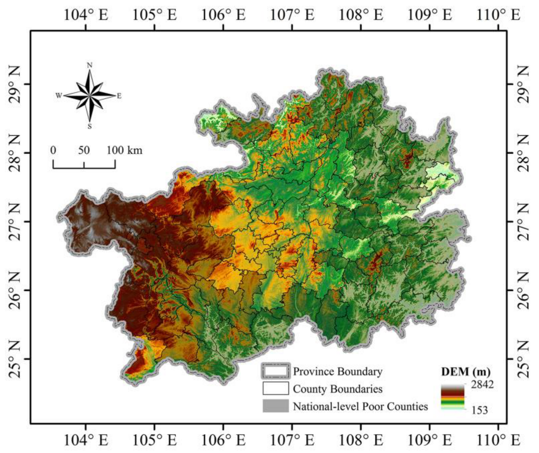
The county is the most basic administrative unit in China. The economic development level and spatial distribution pattern of this unit are the visual performances of the status quo of the regional economic development in China [27]. Therefore, we take the county as the basic unit to identify regional poverty. Figure 1 provides a map of administrative division at the county-level in Guizhou and shows its fifty national-level poor counties released by the state council leading group office of poverty-alleviation and development (http://www.cpad.gov.cn) in 2012. The data of administrative boundaries are from National Geomatics Center of China (http://www.resdc.cn). Guizhou Province is located in Southwest China, the eastern part of Yungui Plateau. Mountain and hilly areas account for 90% of the total area, of which 70% are karst landforms. The topography impacts the regional poverty significantly [27]. The poverty line set by the Chinese government is based on the constant price of RMB 2300 per capita in 2011. According to the minimum annual income standard, the incidence of poverty in Guizhou Province reached 26.80% in 2012. Guizhou is faced with an arduous task of poverty reduction.
The study conducts an analysis of poverty identification on a yearly basis starting from 2012. The nighttime light imagery data were provided by the Visible Infrared Imaging Radiometer Suite (VIIRS). VIIRS is one of five instruments onboard the Suomi National Polar-orbiting Partnership (SNPP) satellite platform (https://www.ngdc.noaa.gov/eog/viirs). The spatial resolution and the illumination resolution of VIIRS are 6 times and 250 times those of Defense Meteorological Satellite Program/Operational Linescan System (DMSP/OLS) detector, respectively, and VIIRS has solved the problem of overflow due to over-saturation of the brightness value, giving the captured night images higher resolution and a greater value for a broader scale of research.
Natural topography has been regarded as one of the most important factors that controls the economic development of a county in China [38]. The studies [26,27,38,39] showed that the complex conditions of the geographical environment have a positive driving effect on the spatial distribution of the poverty-stricken counties in China. Therefore, the Digital Elevation Model (DEM) by Shuttle Radar Topography Mission (SRTM) (http://gdex.cr.usgs.gov/gdex), land use coverage, street data were also used. Vegetation fraction, water coverage, and building coverage were selected for land-use dynamic analysis. The vegetation fraction was obtained based on normalized difference vegetation index [40] that was obtained in the Moderate Resolution Imaging Spectroradiometer (MODIS) band analysis (https://modis.gsfc.nasa.gov/data/dataprod/mod13.php). Water coverage and building coverage were extracted based on the albedo of near infrared and visible light bands of Landsat Image (http://earthexplorer.usgs.gov/). The street network information was collected from Open Street Map (OSM) platform (https://www.openstreetmap.org).
2.2. Methodology
2.2.1. SNPP-VIIR Data Processing
In 2012, the Day-Night Band (DNB) of VIIRS sensor mounted on the SNPP satellite began to provide nighttime lights data with higher spatial resolution and better data quality. Compared with the DMSP/OLS data, it represents great improvements in many aspects and is unprecedentedly powerful in nocturnal observation. The drawback of VIIRS is that some of the noise is not filtered. The SNPP-VIIRS sensor has 22 bands in total, and DNB is one of its bands with the wavelengths from 500 nm to 900 nm and a spatial resolution of about 750 m. DNB features high accuracy in radiation measurement and provides on-board calibration to ensure the accuracy and stability of the data. NOAA provides two forms of SNPP-VIIRS DNB data: daily data and synthetic data. Since only the synthetic data in 2015 is available, extra work needs to be done to get the data of other years. The 2015 annual average data has been officially processed, it can be used as masking data to eliminate light anomalies and background noise. We reduced the noise by a combination of median filtering and low threshold denoising [41]. We corrected the geometric errors in the nighttime light imagery [42] and used the maximum threshold method [43] to remove the abnormal values caused by transient light. Finally, we synthesized the processed data into the annual average data.
2.2.2. Identification Features Selection
Given the applications of nighttime lights data and the identification features used in related fields [9,36,44,45,46,47], we adopted 12 statistical and spatial features to extract meaningful information from nighttime light imagery and identify poor counties. The selected features reveal the differences in the quantity, complexity, diversity, and variability of nighttime lights intensities between counties. Three aspects of statistical features were selected to describe the characteristics of the nighttime light distribution in each county: central tendency, degree of dispersion, and distribution features. The central tendency reflects the general data patterns. The dispersion degree reflects the representation of the minority data. The general distribution characteristics of night-time lights in each county can be used to demonstrate the statistical discrepancies between different counties. We also used the identification features that reflect the geographical environment. Topography is an important factor restricting the development of rural economics in China. Seventy percent of the poor counties in China are characterized by poor topographic condition [27]. By contrast, non-poor counties are mainly located in areas with good topographic conditions [38]. Natural topography determines land availability and regional accessibility and further influences the objective environment of wealth creation [27]. Therefore, the topography and reachability were considered as the features. In addition, China is a country undergoing rapid urbanization. The process of urbanization also reflects the regional development [39]. The land use change can describe the process of urbanization. So, we also chose the land use coverage as the identification features. So, the geographical features include the following easily remote-sensed spatial variables: topography, surface coverage, and reachability based on the SRTM DEM, resource satellite remote sensing image, and OSM data. Table 1 summarizes a total of 23 features for poverty identification and their extraction methods.
2.2.3. Machine Learning Method
Classification is an important direction of research on data mining. At present, many machine-learning methods, including mainly single classification algorithms and ensemble learning algorithms, can be used for classification [11]. As an ensemble learning algorithm, Random Forest (RF) has better performance in classification than some other classification algorithms such as Support Vector Machines (SVM), Artificial Neural Network (ANN), and K-Nearest Neighbors (KNN) [48,49,50,51]. RF deals very well with the problems of missing data, non-equilibrium and multi-collinearity in the data set [52]. Currently, it is one of the algorithms with better results in classification and prediction of multi-variate data [53]. This paper used the RF to predict the poverty probability at the county level in Guizhou from 2012 to 2019 based on the 23 classification features. The classification approaches were conducted using the caret and random forest packages in R statistical software.
A RF model is constructed based on randomly generated training sets and multiple decision trees. The classification results of the test sample set are selected based on votes. The specific steps are described as follows:
- The 23 identification features were calculated in each county.
- The bootstrap sampling method [54] was used to randomly sample with replacement from the collected data of poor counties to construct a poverty training sample set with the same number of samples as the original data set. The unselected samples formed a poverty test sample set to measure the recognition error of the decision tree formed by the poverty training set. Two thirds of the samples were used to build the model, while the remaining one third are used as the test set. The sample sets were based on the national-level poor counties of Guizhou in 2012.
- The multiple poverty features were selected as the basis for construction of the decision tree, and the multiple decision trees were built based on multiple training sample sets constructed. According to the principle of the Classification and Regression Trees (CART) algorithm [55], the classification feature with the smallest Gini coefficient was selected from the m features as the branch node, and the optimal cut-point was determined based on the Gini coefficient after the classification feature was split to complete the construction of the CART tree.
- Starting from the root node, following the procedures in Step (3), the greedy algorithm [56] was employed to select the classification features from top to bottom, until the node cannot be split any further. Thus, the decision tree was constructed. The stopping condition was that the remaining sample number of new leaf node was less than 3.
- The above steps were repeated many times to construct multiple decision trees to form a RF.
- When there was a need to classify the sample in the poverty test set, multiple recognition results of the sample were obtained through RF, the conditional probability of recognition result of the sample was calculated, and the Boyer–Moore majority vote algorithm [55] was used to determine the result with the highest probability as the poverty identification result of the sample.
In the RF, the number of decision tree split attributes (mtry) and the number of decision trees (ntree) are two important attributes, which have an important impact on the performance of poverty identification. It is very important for the construction of the model to determine the appropriate values for ntree and mtry. Therefore, the results of the algorithms with different ntree and mtry were compared and analyzed. When mtry was 4, the accurate poverty identification model showed the lowest error rate. When ntree was greater than 300, the increase in the number of decision trees cannot reduce the error rate significantly but would instead reduce the operating efficiency of the model. Based on the above analysis, mtry and ntree are set to 4 and 300, respectively.
The choice of training sets is the key to the accuracy of classification. This paper selected poor counties from the national-level poor counties identified by the Chinese government in 2012, and non-poor counties from other counties identified by the government as non-poverty-stricken counties. During the adjustment and optimization of training sets, the training sets were subjected to 10-fold cross-validation, and the training sets with high accuracy were selected.
The classification result was denoted by the median value of probability, which can reveal the poverty level of each county and reflect the characteristics of relative poverty. Specifically, the closer the probability value is to 1, the greater the probability of the county to be a poor county. To a certain extent, the choice of threshold will have a significant impact on the accuracy and the prediction error of the model. We set the counties with poverty probability over 0.8 as poor counties. Accuracy is assessed by calculating the coincidence rate in space between the identification results and the 2012 government designation. On the premise that better identification results can be obtained for 2012, we used the RF model derived for 2012 to predict poverty probability at the county level of all the nighttime light imagery from 2012 to 2019 and to investigate the relative spatiotemporal patterns of poor counties in Guizhou.
2.2.4. Spatial and Temporal Analysis of Poverty Probability
In the study, Global Moran’s I and Local Indicators of Spatial Association (LISA) are employed to investigate the spatiotemporal dynamics of poor counties. The Global Moran’s Index is calculated by Equation (1), and its values ranges from -1 to 1 [57,58]. The closer it is to 1, the stronger the positive correlation is, while the closer it is to -1, the stronger the negative correlation; if it is close to 0, the correlation is not significant. LISA analysis uses five attributes (high-high, low-low, high-low, low-high, no significant) to describe the correlation of spatial units [59].
where n is the number of calculation units (such as the number of counties), xi is the poverty probability of the ith county, the upper horizontal line represents the mean value, and wij is the spatial symmetric weight.
Spatial clustering of poverty probability at county level is calculated with the Getis-Ord Gi* statistic [60]. The Getis-Ord Gi* statistic is used to identify significant spatial clusters of high (hot spots) and low values (cold spots). High values surrounded by high values are considered as hot spots, and low values surrounded by low values are considered as cold spots. The Gi* is calculated by Equation (2), where the variables represented by letters were the same as those in Equation (1).
3. Results
3.1. Performance of the Poverty Identification
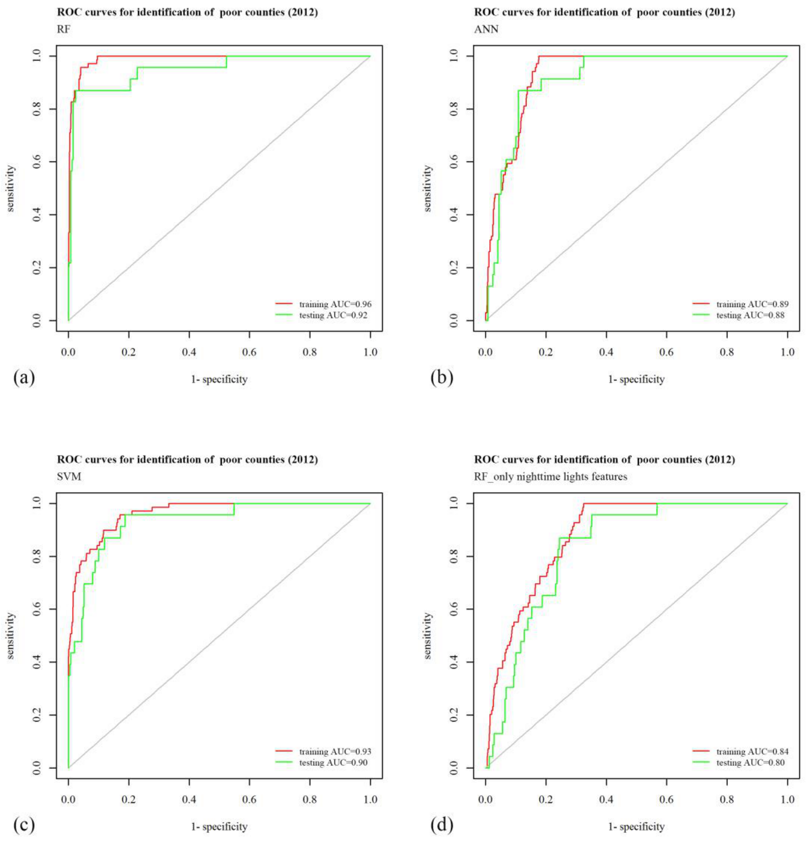
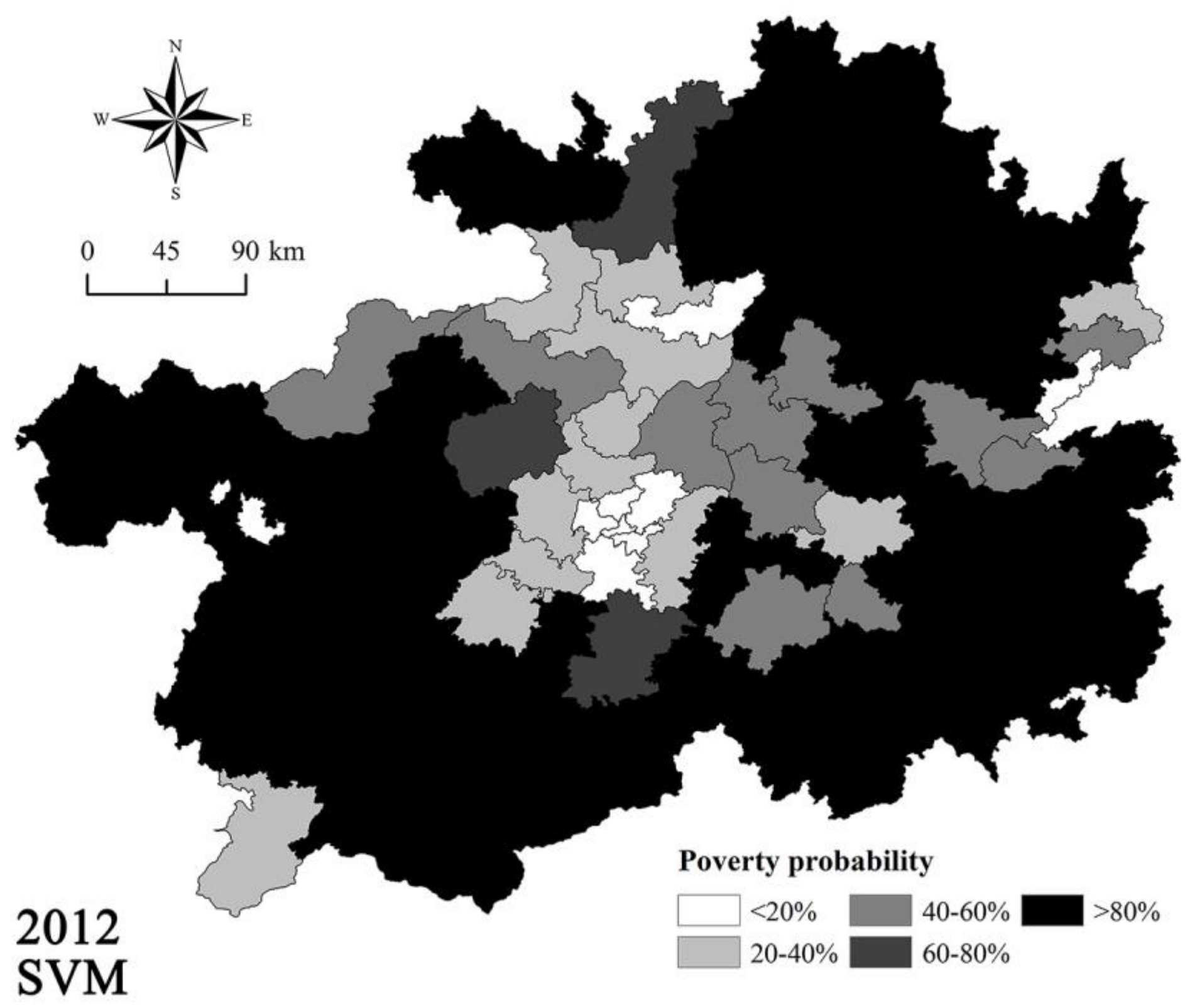
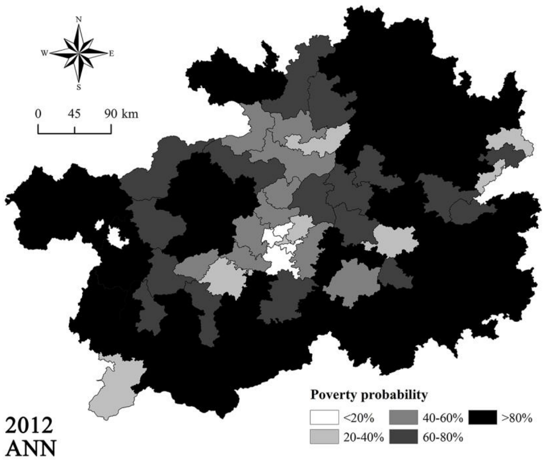
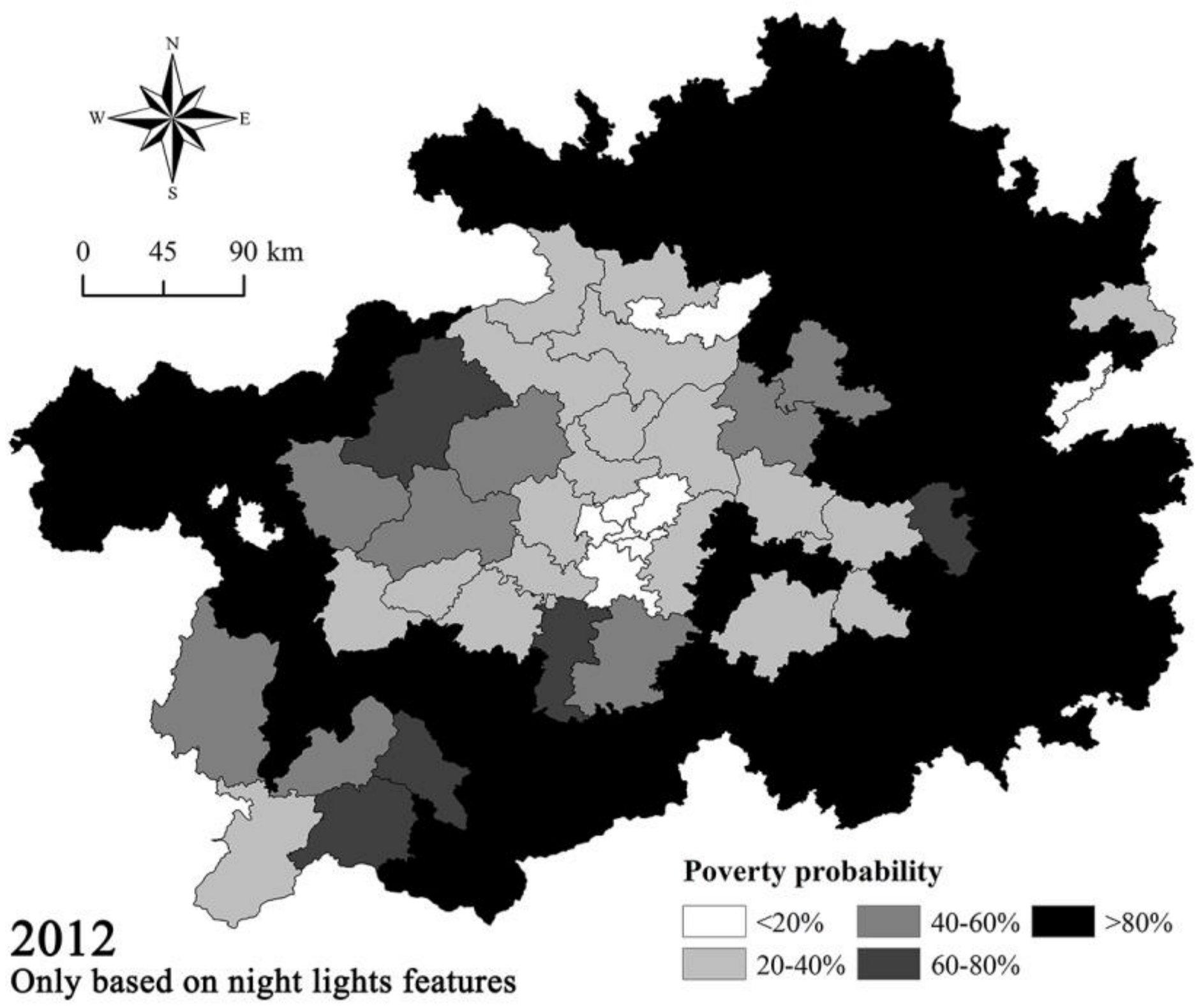
In order to make a comparison between the RF and other machine learning models, we used two typical classification algorithms of SVM and ANN to identify the poverty probability in 2012, and adopted four evaluation indicators, namely, accuracy, precision, recall, and F-value to evaluate the effects of these three models in poverty identification. Table 2 shows the accuracy, precision, recall and F-value of the SVM, ANN, and RF in poverty identification. It also shows the identification results using only nighttime lights features as a comparison. Compared with ANN and SVM, the RF model reaches higher values in its accuracy, precision, recall and F-value, indicating the RF-based identification had a better performance in poverty identification. The performance of the above three methods based on comprehensive features are all higher than that using only nighttime lights features. Figure 2 shows the Receiver Operating Characteristic (ROC) curves of the identification by the four methods. The Area Under Curve (AUC) values from large to small are RF, SVM, ANN, and RF using only nighttime lights features. Therefore, RF is the most reliable among the several schemes tested. The identification results of the above four patterns were shown in Figure 3, Figure 4, Figure 5 and Figure 6.
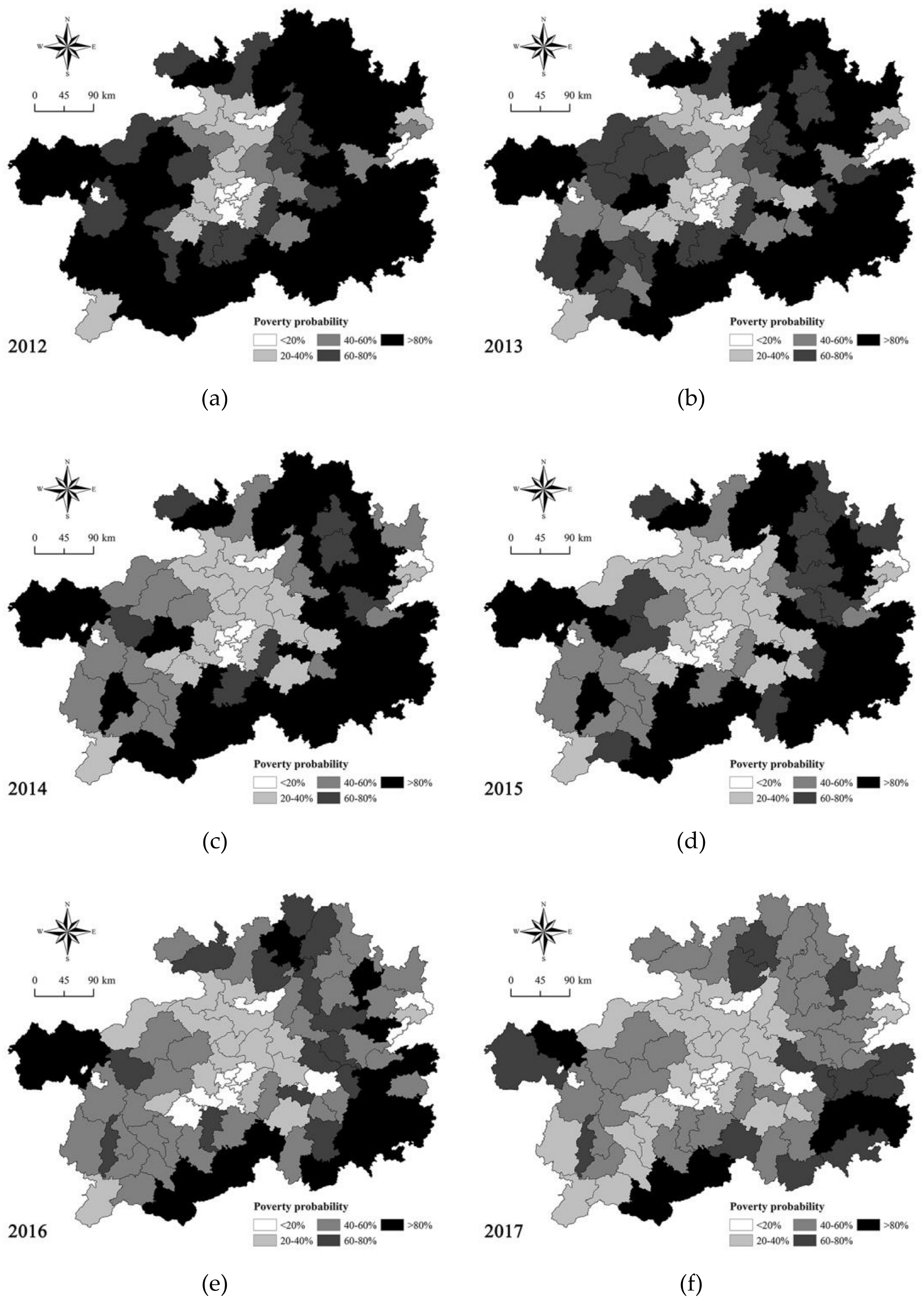
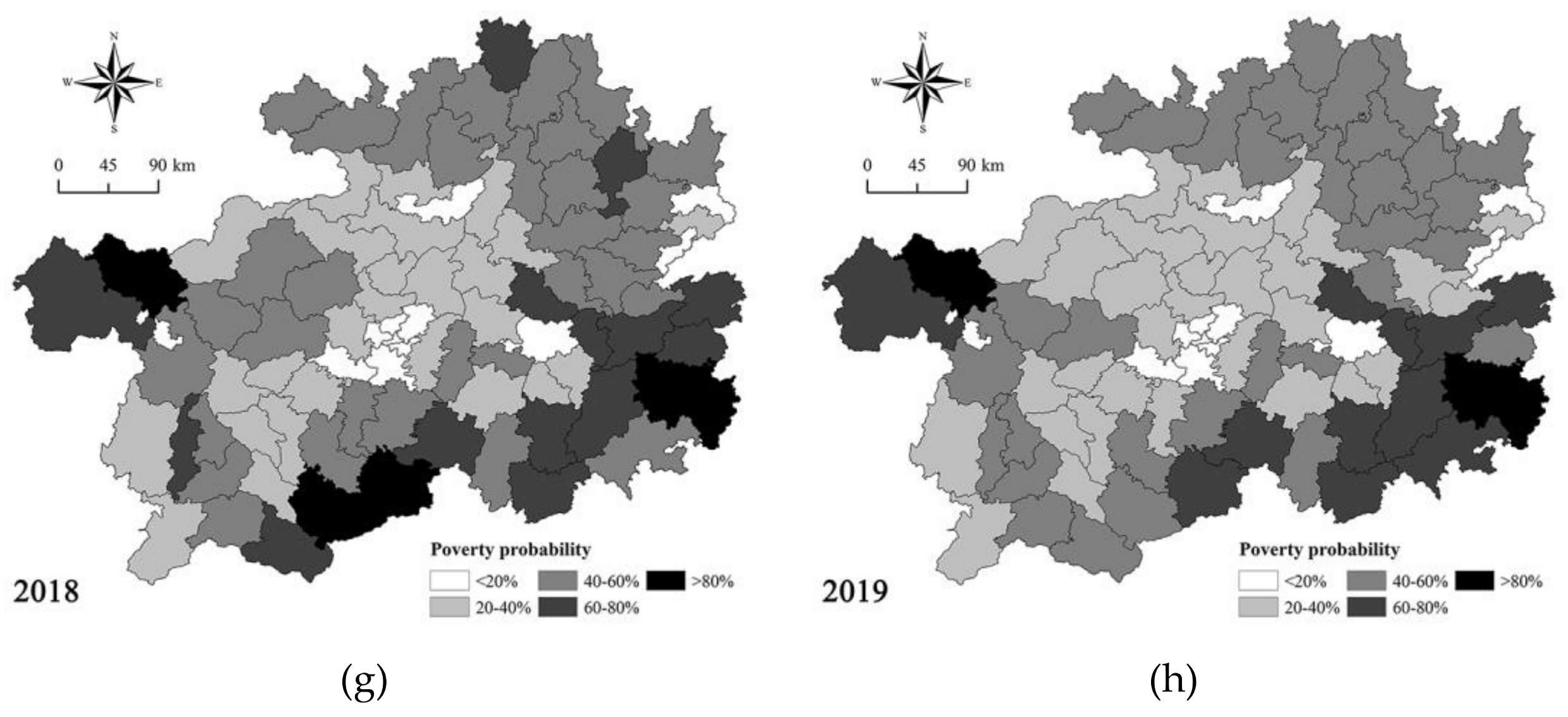
The poverty probability at the county level in 2012 is obtained and compared with the 50 national-level poor counties designated by the Chinese government. Using the RF model, there are 47 counties with a poverty probability greater than 0.8, which is in good agreement with the national-level poor counties. Figure 6 shows the spatiotemporal pattern of poverty probability at the county level in Guizhou from 2012 to 2019. As shown in the figure, there are evident characteristics and dynamics in the spatial distribution of poor counties over time. The poor counties are mainly distributed in the eastern, southern and high-altitude regions of Guizhou. It is obvious that the poor counties of Guizhou are contiguous in distribution. With the support of the poverty-alleviation work, the poor counties have been decreasing. The number of poor counties in the northeast and southwest of Guizhou has declined faster than the number of poor counties in other areas. In terms of the spatial distribution of the poor counties becoming non-poor counties, poor counties that are adjacent to non-poor counties are more easily transformed into non-poor counties. The poverty probability of each county in Guizhou Province changed in fluctuations. The poverty probability of its western region fluctuated greatly, and its eastern and southern regions were consistently recognized as areas with higher poverty probability.
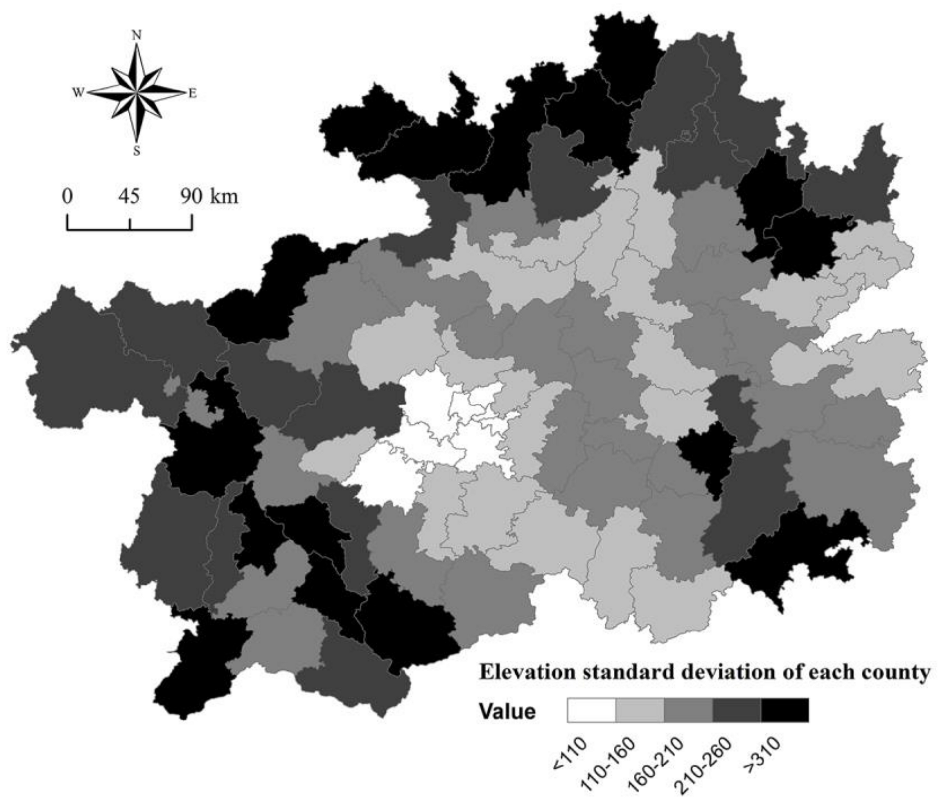
The distribution of poor counties in Guizhou is contiguous, and the spatiotemporal characteristics of contiguous poverty-stricken areas from 2012 to 2019 are evident in Guizhou. The changes in the boundaries of impoverished areas indicate that the spatial distribution of impoverished areas has become more complex, showing obvious regional characteristics. We extracted the spatial distribution characteristics of the topography at the county level (Figure 7 and Figure 8). It is found that the boundary change in the poverty-stricken areas is highly related to the terrain features, and that poverty-alleviation is easier to implement in areas with a high proportion of plains. The plain area in central Guizhou has the lowest incidence of poverty. The area with high altitude and high topographic relief usually has a high incidence of poverty. In addition, the internal fragmentation of the contiguous poverty-stricken areas is intensifying.
3.2. Spatiotemporal Dynamics of Poverty Probability
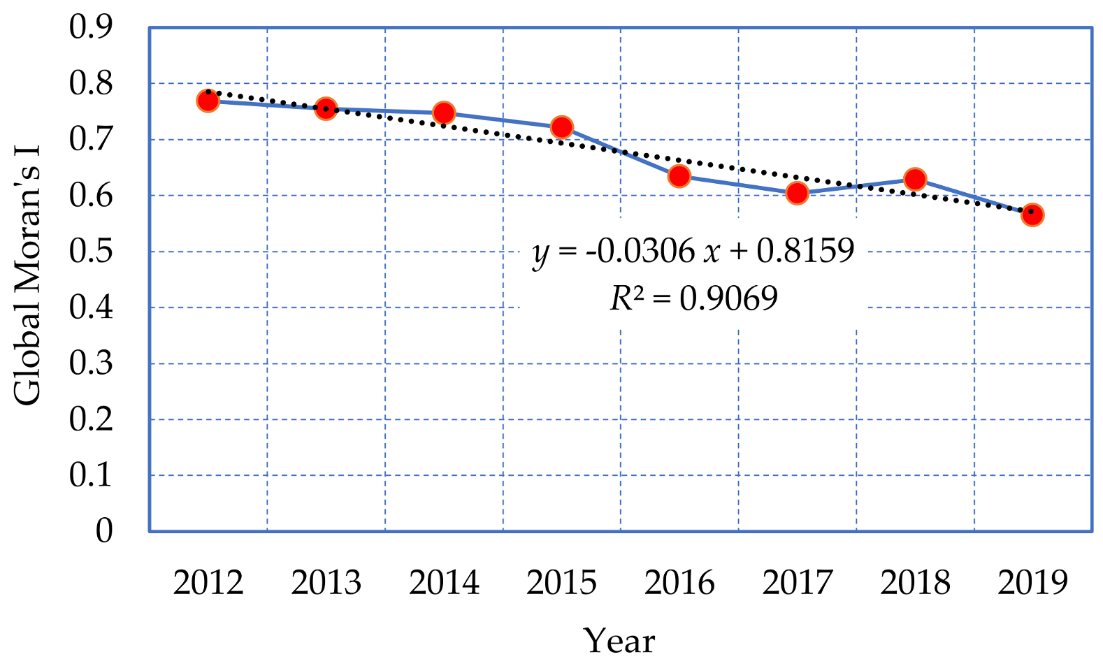
Figure 9 shows the Global Moran’s I of poverty probability at the county level from 2012 to 2019. The results reveal that the estimates of the 8 years are all above 0, indicating that the poverty probability at the county level in Guizhou has a positive spatial autocorrelation. The values are greater than 0.7 from 2012 to 2015, indicating that this spatial autocorrelation is relatively strong during the years. The Global Moran’s I has relatively small fluctuations and a decreasing trend, indicating that the poverty probability at the county level in Guizhou has been relatively stable since 2012 but with a trend of spatial dispersion.
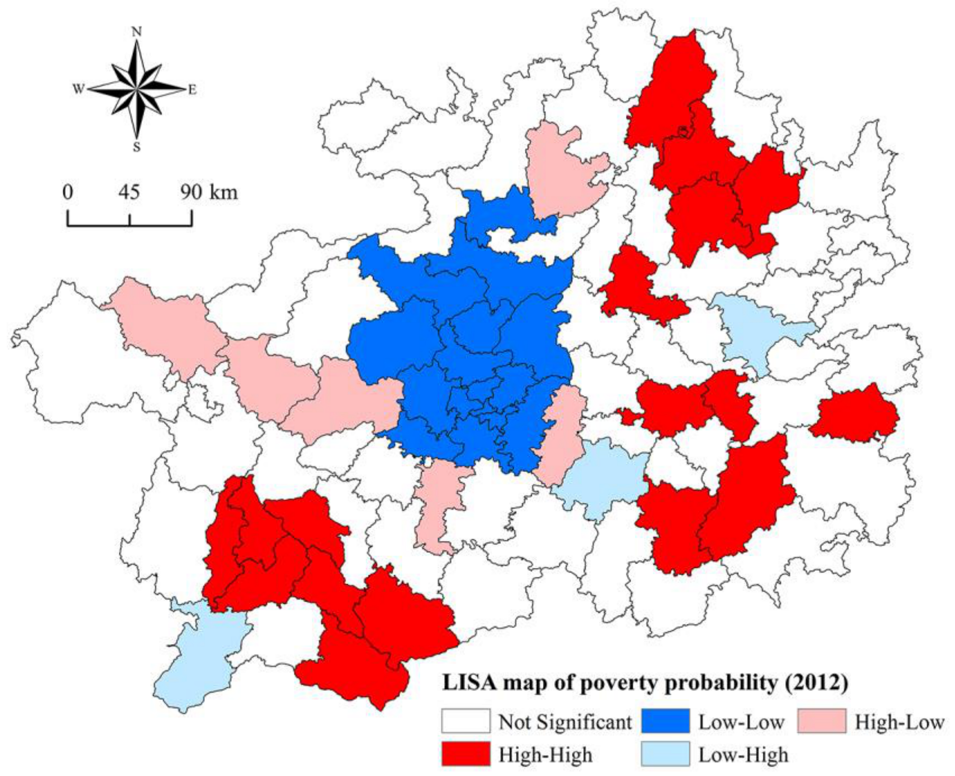
Figure 10 shows the local autocorrelation of poverty probability at the county level in 2012. As shown in the figure, the high-high clusters are primarily located in the eastern and southwestern regions of Guizhou. The central part is identified as having low-low clusters. These results indicate that relatively poor and non-poor counties have obvious regional distribution features. The high-low distribution is mainly found around the low-low clusters, which is related to the rapid poverty-alleviation in this area. The low-high areas were scattered, which were the areas with high possibility of returning to poverty and were also the key areas of poverty-alleviation.
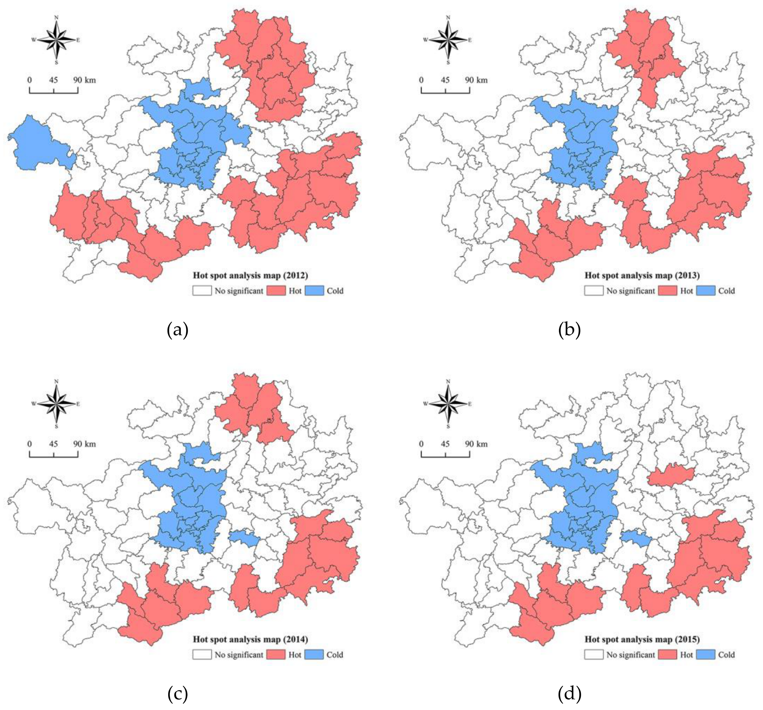
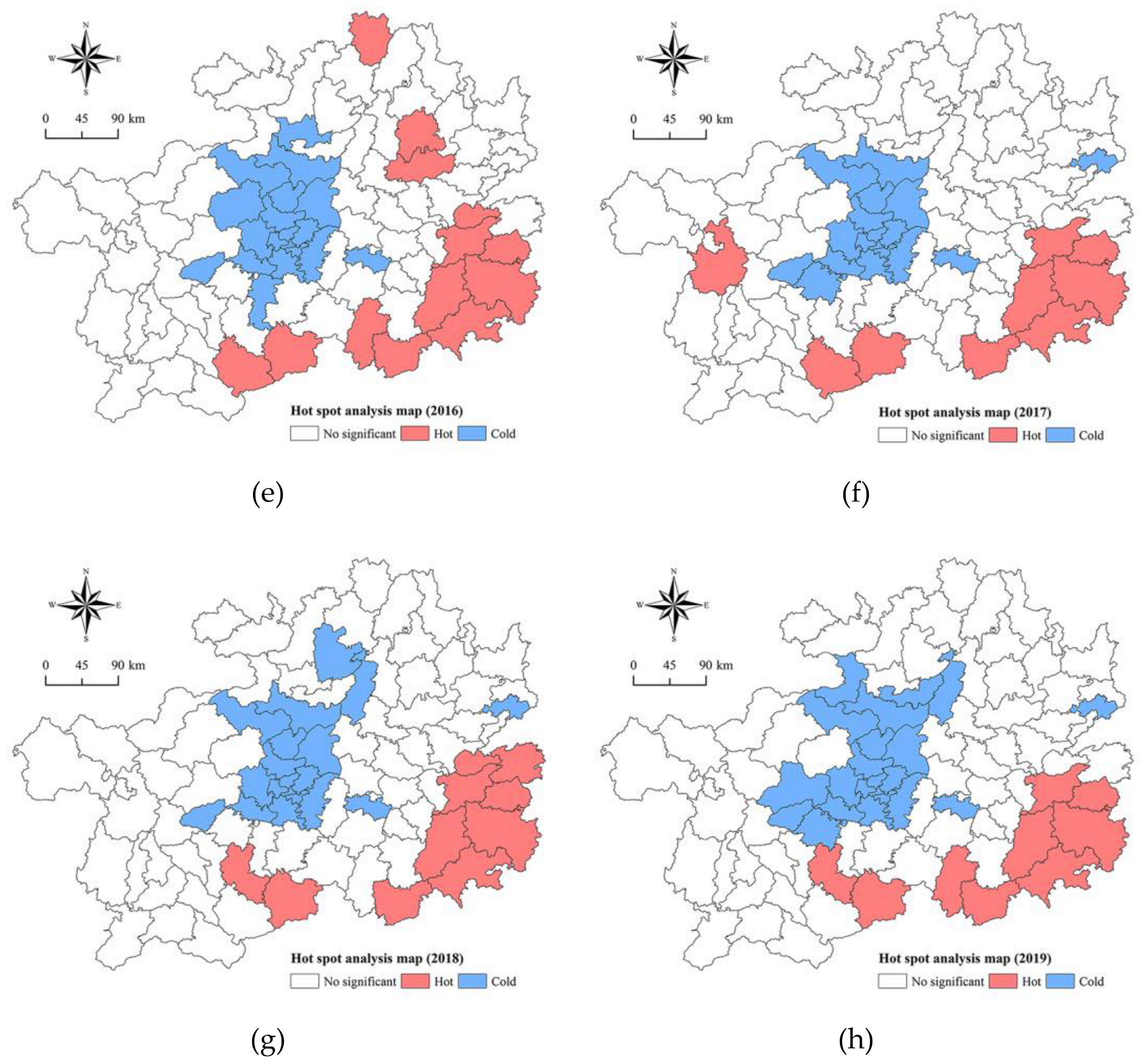
Figure 11 shows the results of the hot spot analysis of poverty in Guizhou. As shown in the figure, the hot spots are mainly distributed in the southeast, southwest, and northeast of Guizhou, while the cold spots are mainly distributed in the central region. After 2016, the poverty hot spots in northeast of Guizhou disappear, indicating that there are no obvious contiguous poverty-stricken areas in the region. Within the whole province, the number of hot spots is decreasing, indicating that the contiguous poverty-stricken areas are gradually shrinking. However, there are still hot spots in southeast and south of Guizhou characterized with spatial agglomeration in 2019. The cold spots gather in the central. It indicates that the southeastern and southwestern parts of Guizhou are the areas with high poverty probability, while the central part of Guizhou has a low poverty probability.
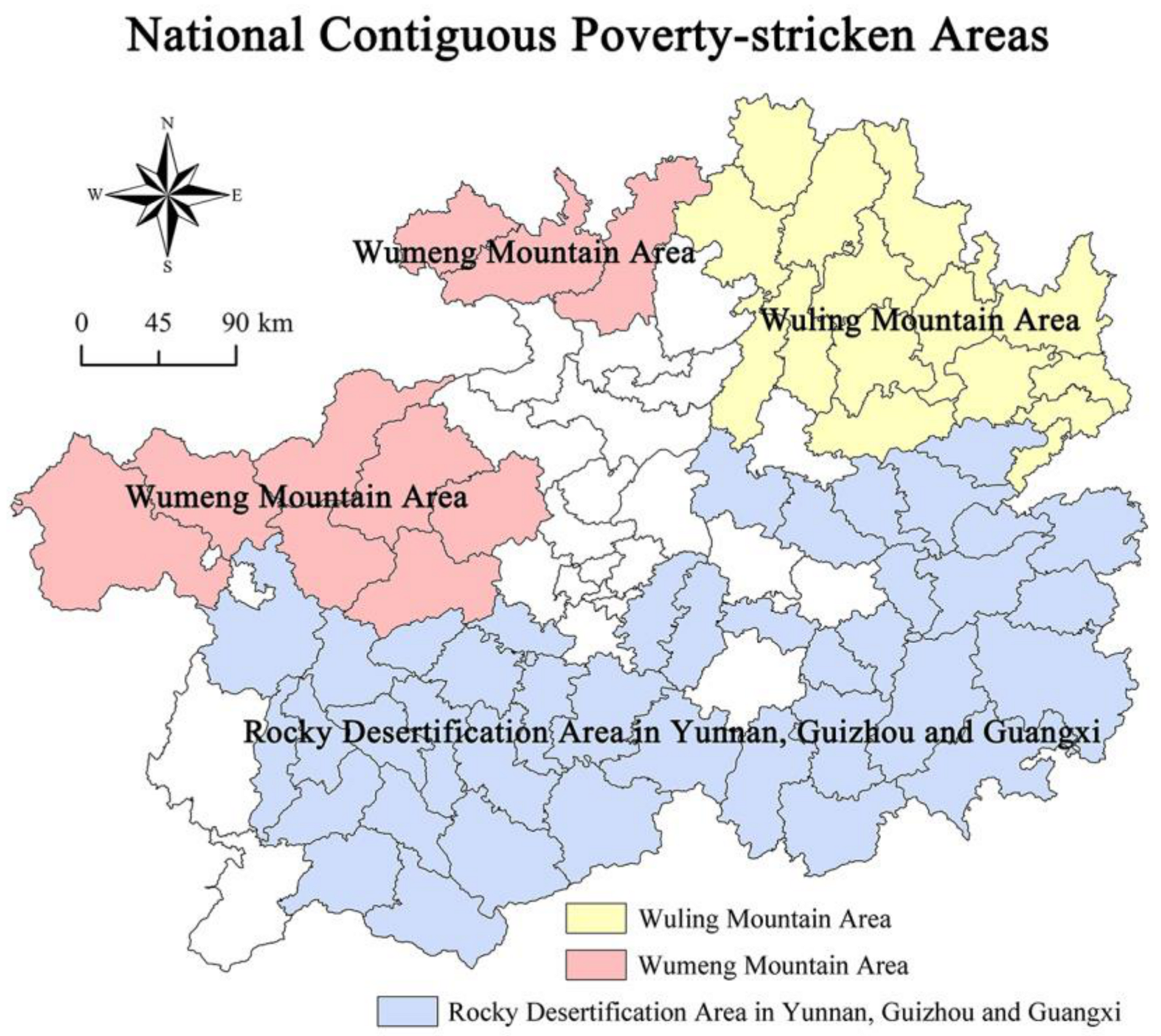
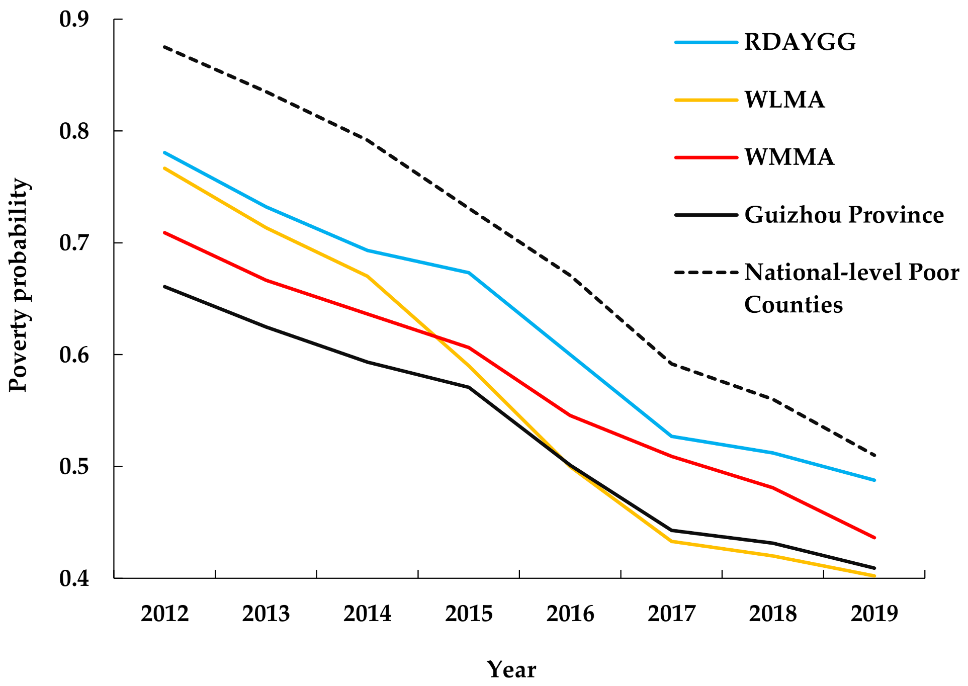
There are three national contiguous poverty-stricken areas (Figure 12) that located in Guizhou partly. They are Wuling Mountain Area (WLMA), Wumeng Mountain Area (WMMA), and Rocky Desertification Area in Yunnan, Guizhou, and Guangxi (RDAYGG). Figure 13 shows the average poverty probability of counties at various regional scales since 2012. The average value of national-level poor counties in Guizhou is greater than that of the WLMA, WMMA, RDAYGG, and the whole province; the average poverty probability of national-level poor counties has approximated that of the whole province; the average value of national-level poor counties is falling faster than that of the whole province. The average value of RDAYGG is far greater than that of the whole province. Since 2016, the average poverty probability of the WLMA has been less than that of the whole province. It indicates the effect of poverty reduction has been remarkable in the region.
4. Discussion and Conclusions
4.1. Poverty Measurement
Poverty is a complex issue that has inextricable relationship with society, economy, environment and so on. It is a global problem and the primary obstacle for the realization of sustainable development. Most of the existing research works rely on statistics data from the government or other organizations, to a certain extent, which has limited the authenticity, validity, and timeliness of poverty-related research, making it difficult to accurately recognize regional poverty and study its dynamic spatiotemporal characteristics. Nighttime light imagery data provides abundant poverty-related information that improves the efficiency of poverty identification. However, it is also insufficient to rely merely on nighttime lights remote sensing data. Poverty is a comprehensive problem, and poverty identification may be affected by indicators such as topography and environment. Considering that the geographical conditions of Guizhou are the important reason for poverty, this paper extracted 23 spatial features including nighttime light imagery data and geographical data and carried out the poverty identification at the county level in Guizhou since 2012. Compared with the results of the study using only nighttime lights remote sensing data, the accuracy has been improved. Therefore, it is necessary to introduce geographical data into poverty identification. Our results provide an approximate description of the variation of poor counties in Guizhou from 2012 to 2019 and identify the regions that were impoverished in these years. As an exploratory study, our research represents the attempt to estimate poverty only using remote-sensed data. We hope that our research can serve as a reference for future researchers and facilitate more accurately targeted antipoverty strategies.
4.2. Spatiotemporal Dynamics of Poverty
Poor counties present obvious spatiotemporal dynamics in Guizhou from 2012 to 2019. The number of poor counties fluctuates but overall decreases over time. The non-poor counties are mainly distributed in the central part of Guizhou, while the poor counties are mainly distributed in the southwestern, southeastern and northwestern regions. Geographical barriers hinder or limit regional development and are an important cause of poverty. The reduction of poor counties started from the central and northern regions in Guizhou and spread to the periphery. Affected by the topography, poverty reduction is relatively slow in areas with large slope and large topographic relief. When poor counties are adjacent to more non poor counties, it is easier for them to get rid of poverty. The results are consistent with the law of regional development and practical conditions.
In order to study the dynamic changes in the poverty-alleviation phases of Guizhou and the impact of the phased policies on the distribution of poor counties, we further analyzed the poor counties at some important phases. In the year of 2016, China over fulfilled the goal of reducing rural poverty by 10 million with the support of national policies, which was a milestone in the history of poverty alleviation in China. Figure 6 shows the number of counties with a poverty probability greater than 80% decrease significantly in 2016, reflecting the poverty-alleviation achievements. The Chinese government pointed out that 2019 was a crucial year to win the fight against poverty. As shown in Figure 6, the poverty probability in Guizhou is greatly reduced in 2019, and there are only three counties with a poverty probability greater than 80%. These findings reveal that the regional economic development and national policy implementation are highly related to the spatiotemporal dynamics of poverty, and the key to achieving regional poverty reduction is the development of the regional economy and the implementation of national macrolevel policies. Therefore, the results of the spatiotemporal dynamic of poverty can be used to make targeted policies for poverty reduction in impoverished areas, to achieve more sustainable and effective poverty-alleviation.
4.3. Applications and Implications
Compared with research that relies on census and commercial data sets, machine learning method based on remote sensing data can effectively improve the efficiency of poverty identification while allowing for real-time monitoring. As nighttime light imagery data and other remote sensing data are accessible at any time for free, the cost of poverty identification can be greatly reduced. This method can cope with the problems of lack of statistical information and high statistical costs and can serve as a reference for poverty surveys and targeted poverty alleviation in regional and even global underdeveloped areas.
The county is the most basic administrative unit in China and around the world. The economic development and spatial distribution pattern of this unit are the visual performances of the status quo of the regional economic development in China [27]. Therefore, the poverty analysis at the county level could support the regional coordinated development and the national macrolevel formulation of policies.
4.4. Limitations and Prospects
Nighttime light imagery data is a kind of comprehensive information. In the future, the exploration could be made to build a correlation model between geographical characteristics and nighttime lights data, and analyze whether certain features of nighttime lights data can replace the geographical data. In addition, limited by the available verification data, this study only verified the results in 2012. The RF with higher accuracy than ANN and SVM was used to identify the poverty probability after 2012. It needs to consider that the best RF for poverty probability identification may change over time. Therefore, the results may not be the most accurate identification by using the RF of 2012 in the next few years. Finally, this study only qualitatively discusses the correlation between geographical factors and poverty. Future research will focus on geostatistical analysis to examine multiple factors affecting poverty identification quantitatively.
Author Contributions
Conceptualization, Jian Yin; methodology, Jian Yin; validation, Jian Yin, Yuanhong Qiu and Bin Zhang; formal analysis, Jian Yin; investigation, Jian Yin; resources, Bin Zhang; data curation, Jian Yin; writing—original draft preparation, Jian Yin; writing—review and editing, Jian Yin and Bin Zhang; visualization, Jian Yin and Yuanhong Qiu. All authors have read and agreed to the published version of the manuscript.
Funding
This work was partially supported by the MOE (Ministry of Education in China) Liberal arts and Social Sciences Foundation (Grant No. 19YJCZH228), and the University Project of Guizhou University of Finance and Economics (2019XJC03). The authors are grateful to the reviewers for the help and thought-provoking comments.
Informed Consent Statement
Not applicable.
Data Availability Statement
The data presented in this study are available on request from the corresponding author.
Acknowledgments
We thank the editors and the anonymous reviewers for their valuable comments and suggestions.
Conflicts of Interest
The authors declare no conflict of interest.
References
- Zhao, X.; Yu, B.; Liu, Y.; Chen, Z.; Li, Q.; Wang, C.; Wu, J. Estimation of poverty using random forest regression with multi-source data: A case study in Bangladesh. Remote Sens. 2019, 11, 375. [Google Scholar] [CrossRef] [Green Version]
- Lo, K.; Wang, M. How voluntary is poverty-alleviation resettlement in China? Habitat Int. 2018, 73, 34–42. [Google Scholar] [CrossRef]
- Sun, J.; Xia, T. China’s Anti-poverty strategy and post-2020 relative poverty line. China Econ. 2020, 15, 62–75. [Google Scholar] [CrossRef]
- Guo, Y.; Zhou, Y.; Cao, Z. Geographical patterns and anti-poverty targeting post-2020 in China. J. Geogr. Sci. 2018, 28, 1810–1824. [Google Scholar] [CrossRef]
- Wu, Y.; Qi, D. A gender-based analysis of multidimensional poverty in China. Asian J. Womens Stud. 2017, 23, 66–88. [Google Scholar] [CrossRef]
- Luo, G.; Wang, B.; Luo, D.; Wei, C. Spatial agglomeration characteristics of rural settlements in poor mountainous areas of Southwest China. Sustainability 2020, 12, 1818. [Google Scholar] [CrossRef] [Green Version]
- Yang, L.; Jiang, C.; Ren, X.; Walker, R.; Xie, J.; Zhao, Y. Determining Dimensions of Poverty Applicable in China: A Qualitative Study in Guizhou. J. Soc. Serv. Res. 2020, 1–18. [Google Scholar] [CrossRef]
- Xu, Z.; Cai, Z.; Wu, S.; Huang, X.; Liu, J.; Sun, J.; Su, S.; Weng, M. Identifying the geographic indicators of poverty using geographically weighted rgression: A case study from Qiandongnan Miao and Dong Autonomous Prefecture, Guizhou, China. Soc. Indic. Res. 2019, 142, 947–970. [Google Scholar] [CrossRef]
- Li, G.; Chang, L.; Liu, X.; Su, S.; Cai, Z.; Huang, X.; Li, B. Monitoring the spatiotemporal dynamics of poor counties in China: Implications for global sustainable development goals. J. Clean. Prod. 2019, 227, 392–404. [Google Scholar] [CrossRef]
- Labar, K.; Bresson, F. A multidimensional analysis of poverty in China from 1991 to 2006. China Econ. Rev. 2011, 22, 646–668. [Google Scholar] [CrossRef]
- Jean, N.; Burke, M.; Xie, M.; Davis, W.M.; Lobell, D.B.; Ermon, S. Combining satellite imagery and machine learning to predict poverty. Science 2016, 353, 790–794. [Google Scholar] [CrossRef] [PubMed] [Green Version]
- Hick, R. Material poverty and multiple deprivation in Britain: The distinctiveness of multidimensional assessment. J. Public Policy 2016, 36, 277–308. [Google Scholar] [CrossRef]
- Yu, B.; Shi, K.; Hu, Y.; Huang, C.; Chen, Z.; Wu, J. Poverty evaluation using NPP-VIIRS nighttime light composite data at the county level in China. IEEE J. Sel. Top. Appl. Earth Obs. Remote Sens. 2017, 8, 1217–1229. [Google Scholar] [CrossRef]
- Njuguna, C.; McSharry, P. Constructing spatiotemporal poverty indices from big data. J. Bus. Res. 2017, 70, 318–327. [Google Scholar] [CrossRef]
- Elvidge, C.D.; Ziskin, D.; Baugh, K.E.; Tuttle, B.T.; Ghosh, T.; Pack, D.W.; Erwin, E.H.; Zhizhin, M. A fifteen year record of global natural gas flaring derived from satellite data. Energies 2009, 2, 595–622. [Google Scholar] [CrossRef]
- Bunte, J.B.; Desai, H.; Gbala, K.; Parks, B.; Runfola, D.M. Natural resource sector FDI, government policy, and economic growth: Quasi-experimental evidence from Liberia. World Dev. 2018, 107, 151–162. [Google Scholar] [CrossRef]
- Kuffer, M.; Pfeffer, K.; Sliuzas, R. Slums from space—15 years of slum mapping using remote sensing. Remote Sens. 2016, 8, 455. [Google Scholar] [CrossRef] [Green Version]
- Mahabir, R.; Croitoru, A.; Crooks, A.T.; Agouris, P.; Stefanidis, A. A critical review of high and very high-resolution remote sensing approaches for detecting and mapping slums: Trends, challenges and emerging opportunities. Urban Sci. 2018, 2, 8. [Google Scholar] [CrossRef] [Green Version]
- Wurm, M.; Stark, T.; Zhu, X.X.; Weigand, M.; Taubenboeck, H. Semantic segmentation of slums in satellite images using transfer learning on fully convolutional neural networks. ISPRS J. Photogramm. Remote Sens. 2019, 150, 59–69. [Google Scholar] [CrossRef]
- Wurm, M.; Taubenbck, H.; Weigand, M.; Schmitt, A. Slum mapping in polarimetric SAR data using spatial features. Remote Sens. Environ. 2017, 194, 190–204. [Google Scholar] [CrossRef]
- Mast, J.; Wei, C.; Wurm, M. Mapping urban villages using fully convolutional neural networks. Remote Sens. Lett. 2020, 11, 630–639. [Google Scholar] [CrossRef]
- Engstrom, R.; Hersh, J.; Newhouse, D. Poverty from Space: Using High-Resolution Satellite Imagery for Estimating Economic Well-Being. World Bank Policy Res. Work. Pap. 2017, 8284. [Google Scholar] [CrossRef]
- Wurm, M.; Taubenböck, H. Detecting social groups from space—Assessment of remote sensing-based mapped morphological slums using income data. Remote Sens. Lett. 2018, 9, 41–50. [Google Scholar] [CrossRef]
- Hannes, T.; Jeroen, S.; Xiao, Z.; Christian, G.; Stefan, D.; Michael, W. Are the poor digitally left behind? Indications of urban divides based on remote sensing and twitter data. ISPRS Int. J. Geo Inf. 2018, 7, 304. [Google Scholar] [CrossRef] [Green Version]
- Niu, T.; Chen, Y.; Yuan, Y. Measuring urban poverty using multi -source data and a random forest algorithm: A case study in Guangzhou. Sustain. Cities Soc. 2020, 54, 102014. [Google Scholar] [CrossRef]
- Liu, Y.; Liu, J.; Zhou, Y. Spatio-temporal patterns of rural poverty in China and targeted poverty-alleviation strategies. J. Rural Stud. 2017, 52, 66–75. [Google Scholar] [CrossRef]
- Zhou, L.; Xiong, L. Natural topographic controls on the spatial distribution of poverty-stricken counties in China. Appl. Geogr. 2018, 90, 282–292. [Google Scholar] [CrossRef]
- National Bureau of Statistics. Available online: http://www.stats.gov.cn/tjsj/zxfb/201908/t20190829_1694202.html (accessed on 10 December 2020).
- Ren, Q.; Huang, Q.; He, C.; Tu, M.; Liang, X. The poverty dynamics in rural china during 2000–2014: A multi-scale analysis based on the poverty gap index. J. Geogr. Sci. 2018, 28, 1427–1443. [Google Scholar] [CrossRef] [Green Version]
- Huang, Q.; Yang, X.; Gao, B.; Wang, L.; Hu, Y.; Wang, J.; Huang, W. Application of DMSP/OLS nighttime light images: A meta-analysis and a systematic literature review. Remote Sens. 2014, 6, 6844–6866. [Google Scholar] [CrossRef] [Green Version]
- Keola, S.; Andersson, M.; Hall, O. Monitoring economic development from space: Using nighttime light and land cover data to measure economic growth. World Dev. 2015, 66, 322–334. [Google Scholar] [CrossRef]
- Shao, S.; Tian, Z.; Fan, M. Do the rich have stronger willingness to pay for environmental protection? New evidence from a survey in China. World Dev. 2018, 105, 83–94. [Google Scholar] [CrossRef]
- Wang, W.; Cheng, H.; Zhang, L. Poverty assessment using DMSP/OLS night-time light satellite imagery at a provincial scale in China. Adv. Space Res. 2012, 49, 1253–1264. [Google Scholar] [CrossRef]
- Pan, W.; Fu, H.; Zheng, P. Regional poverty and inequality in the Xiamen-Zhangzhou-Quanzhou city cluster in China based on NPP/VIIRS night-time light imagery. Sustainability 2020, 12, 2547. [Google Scholar] [CrossRef] [Green Version]
- Shi, K.; Chang, Z.; Chen, Z.; Wu, J.; Yu, B. Identifying and evaluating poverty using multisource remote sensing and point of interest (POI) data: A case study of Chongqing, China. J. Clean Prod. 2020, 255, 120245. [Google Scholar] [CrossRef]
- Li, G.; Cai, Z.; Liu, X.; Liu, J.; Su, S. A comparison of machine learning approaches for identifying high-poor counties: Robust features of DMSP/OLS night-time light imagery. Int. J. Remote Sens. 2019, 40, 5716–5736. [Google Scholar] [CrossRef]
- Xu, J.; Song, J.; Cao, X.; Sun, F. Spatial pattern of poverty and its influencing factors Based on CART Model in Guizhou Province. Econ. Geogr. 2020, 40, 166–173. [Google Scholar] [CrossRef]
- Ward, P.S. Transient poverty, poverty dynamics, and vulnerability to Poverty: An empirical analysis using a balanced panel from rural China. World Dev. 2016, 78, 541–553. [Google Scholar] [CrossRef] [Green Version]
- Zhang, K.; Dearing, J.A.; Dawson, T.P.; Dong, X.; Yang, X.; Zhang, W. Poverty-alleviation strategies in eastern china lead to critical ecological dynamics. Sci. Total Environ. 2015, 506–507, 164–181. [Google Scholar] [CrossRef] [Green Version]
- Gong, Z.; Zhao, S.; Gu, J. Correlation analysis between vegetation coverage and climate drought conditions in North China during 2001–2013. J. Geogr. Sci. 2017, 27, 143–160. [Google Scholar] [CrossRef]
- Zhong, L.; Liu, X.; Yang, P. Method for SNPP-VIIRS nighttime lights images denoising. Bull. Surv. Mapp. 2019, 3, 21–26. [Google Scholar] [CrossRef]
- Wang, W.; Cao, C.; Bai, Y.; Blonski, S.; Schull, M.A. Assessment of the NOAA S-NPP VIIRS geolocation reprocessing improvements. Remote Sens. 2017, 9, 974. [Google Scholar] [CrossRef] [Green Version]
- Chen, Z.; Yu, B.; Hu, Y.; Huang, C.; Shi, K.; Wu, J. Estimating house vacancy rate in metropolitan areas using NPP-VIIRS nighttime light composite data. IEEE J. Sel. Top. Appl. Earth Obs. Remote Sens. 2015, 8, 2188–2197. [Google Scholar] [CrossRef]
- Li, X.; Ge, L.; Chen, X. Detecting Zimbabwe’s decadal economic decline using nighttime light imagery. Remote Sens. 2013, 5, 4551–4570. [Google Scholar] [CrossRef] [Green Version]
- Small, C.; Elvidge, C.D. Night on earth: Mapping decadal changes of anthropogenic night light in Asia. Int. J. Appl. Earth Obs. Geo Inf. 2013, 22, 40–52. [Google Scholar] [CrossRef] [Green Version]
- Wu, J.; Wang, Z.; Li, W.; Peng, J. Exploring factors affecting the relationship between light consumption and GDP based on DMSP/OLS nighttime satellite imagery. Remote Sens. Environ. 2013, 134, 111–119. [Google Scholar] [CrossRef]
- Ma, T.; Zhou, Y.; Zhou, C.; Haynie, S.; Pei, T.; Xu, T. Night-time light derived estimation of spatio-temporal characteristics of urbanization dynamics using DMSP/OLS satellite data. Remote Sens. Environ. 2015, 158, 453–464. [Google Scholar] [CrossRef]
- You, H.; Ma, Z.; Tang, Y.; Wang, Y.; Yan, J.; Ni, M.; Cen, K.; Huang, Q. Comparison of ANN (MLP), ANFIS, SVM, and RF models for the online classification of heating value of burning municipal solid waste in circulating fluidized bed incinerators. Waste Manag. 2017, 68, 186. [Google Scholar] [CrossRef]
- Yuan, H.; Yang, G.; Li, C.; Wang, Y.; Liu, J.; Yu, H.; Feng, H.; Xu, B.; Zhao, X.; Yang, X. Retrieving soybean leaf area index from unmanned aerial vehicle hyperspectral remote sensing: Analysis of RF, ANN, and SVM regression models. Remote Sens. 2017, 9, 309. [Google Scholar] [CrossRef] [Green Version]
- Sun, T.; Chen, F.; Zhong, L.; Liu, W.; Wang, Y. GIS-based mineral prospectivity mapping using machine learning methods: A case study from Tongling ore district, eastern China. Ore Geol. Rev. 2019, 109, 26–49. [Google Scholar] [CrossRef]
- Luo, L. Reserch on targeted poverty indentification model based on random forest algorithms. J. Huazhong Agric. Univ. 2019, 144, 21–29. [Google Scholar] [CrossRef]
- Mutanga, O.; Adam, E.; Cho, M.A. High density biomass estimation for wetland vegetation using WorldView-2 imagery and random forest regression algorithm. Int. J. Appl. Earth Obs. Geoinf. 2012, 18, 399–406. [Google Scholar] [CrossRef]
- Stumpf, A.; Kerle, N. Object-oriented mapping of landslides using random forests. Remote Sens. Environ. 2011, 115, 2564–2577. [Google Scholar] [CrossRef]
- Rodriguez-Galiano, V.F.; Ghimire, B.; Rogan, J.; Chica-Olmo, M.; Rigol-Sanchez, J.P. An assessment of the effectiveness of a random forest classifier for land-cover classification. ISPRS J. Photogramm. Remote Sens. 2012, 67, 93–104. [Google Scholar] [CrossRef]
- Breiman, L. Random forests. Mach. Learn. 2001, 45, 5–32. [Google Scholar] [CrossRef] [Green Version]
- Halstead, J.B. Recruiter selection model and implementation within the United States Army. IEEE Trans. Syst. Man Cybern. Part C 2009, 39, 93–100. [Google Scholar] [CrossRef]
- Moran, P.A.P. The interpretation of statistical maps. J. R. Stat. Soc. Ser. B Stat. Methodol. 1948, 10, 243–251. [Google Scholar] [CrossRef]
- Su, S.; Zhou, H.; Xu, M.; Ru, H.; Wang, W.; Weng, M. Auditing street walkability and associated social inequalities for planning implications. J. Transp. Geogr. 2019, 74, 62–76. [Google Scholar] [CrossRef]
- Su, S.; Pi, J.; Xie, H.; Cai, Z.; Weng, M. Community deprivation, walkability, and public health: Highlighting the social inequalities in land use planning for health promotion. Land Use Policy 2017, 67, 315–326. [Google Scholar] [CrossRef]
- Songchitruksa, P.; Zeng, X. Getis–Ord spatial statistics to identify hot spots by using incident management data. Transp. Res. Rec. 2010, 2165, 42–51. [Google Scholar] [CrossRef]
Figure 1.
Distribution of the national-level poor counties of Guizhou in 2012.

Figure 2.
The Receiver Operating Characteristic (ROC) curves of poor counties identification in 2012. (a) ROC curves of poor counties identification by RF, (b) ROC curves of poor counties identification by ANN, (c) ROC curves of poor counties identifi-cation by SVM, (d) ROC curves of poor counties identifi-cation by RF_only nighttime lights fea-tures.

Figure 3.
Distribution of poverty probability at the county level by Support Vector Machines (SVM) in 2012.
Figure 3.
Distribution of poverty probability at the county level by Support Vector Machines (SVM) in 2012.

Figure 4.
Distribution of poverty probability at the county level by the Artificial Neural Network (ANN) in 2012.
Figure 4.
Distribution of poverty probability at the county level by the Artificial Neural Network (ANN) in 2012.

Figure 5.
Distribution of poverty probability at the county level by Random Forest (RF) only based on nighttime lights features in 2012.
Figure 5.
Distribution of poverty probability at the county level by Random Forest (RF) only based on nighttime lights features in 2012.

Figure 6.
Distribution of poverty probability at the county level by RF from 2012 to 2019, (a) poverty probability at the county level by RF in 2012, (b) poverty probability at the county level by RF in 2013, (c) poverty probability at the county level by RF in 2014, (d) poverty probability at the county level by RF in 2015, (e) poverty probability at the county level by RF in 2016, (f) poverty probability at the county level by RF in 2017, (g) poverty probability at the county level by RF in 2018, (h) poverty probability at the county level by RF in 2019.


Figure 7.
Distribution of elevation standard deviation at the county level.

Figure 8.
Distribution of average slope at the county level.

Figure 9.
Global Moran’s I of poverty probability from 2012 to 2019 in Guizhou Province.

Figure 10.
Local Indicators of Spatial Association (LISA) map of poverty probability at the county level for 2012.
Figure 10.
Local Indicators of Spatial Association (LISA) map of poverty probability at the county level for 2012.

Figure 11.
Hot-cold spot map of poverty probability at the county level; (a) hot-cold spot analysis map of poverty probability at the county level in 2012, (b) hot-cold spot analysis map of poverty probability at the county level in 2013, (c) hot-cold spot analysis map of poverty probability at the county level in 2014, (d) hot-cold spot analysis map of poverty probability at the county level in 2015, (e) hot-cold spot analysis map of poverty probability at the county level in 2016, (f) hot-cold spot analysis map of poverty probability at the county level in 2017, (g) hot-cold spot analysis map of poverty probability at the county level in 2018, (h) hot-cold spot analysis map of poverty probability at the county level in 2019.


Figure 12.
Distribution of national contiguous poverty-stricken areas of Guizhou Province.

Figure 13.
Average poverty probability from 2012 to 2019 at different spatial scales.


Table 1.
Description of feature variables.
| Feature Types | Aspects | Descriptions and Statistical Methods | Data Sources |
|---|---|---|---|
| Nighttime lights | Central tendency | Average of all pixels of the nighttime lights within the county’s boundary | SNPP-VIIRS |
| Median value of all pixels within the county’s boundary | |||
| Average light index of all pixels within the county’s boundary | |||
| Dispersion degree | Variance of all pixels within the county’s boundary | ||
| Standard deviation of all pixels within the county’s boundary | |||
| Sum of squares of deviation of all pixels within the county’s boundary | |||
| Distribution characteristics | Total value of all pixels within the county’s boundary | ||
| Number of pixels within the county’s boundary | |||
| Number of pixels greater than zero within the county’s boundary | |||
| Largest value of all pixels within the county’s boundary | |||
| Smallest value of all pixels within the county’s boundary | |||
| Range between the largest and smallest value of all pixels within the county’s boundary | |||
| Topography | Elevation | Standard deviation of all pixels of the elevation within the county’s boundary | SRTM DEM |
| Average of all pixels of the elevation within the county’s boundary | |||
| Slope | Average of all pixels of the slope data within the county’s boundary | ||
| Percentage of pixels with slope greater than 20 degree within the county’s boundary | |||
| Surface coverage | Vegetation coverage | Average of all pixels of vegetation fraction within the county’s boundary | MODIS/Landsat |
| water coverage | Percentage of water coverage within the county’s boundary | ||
| Building coverage | Percentage of building coverage within the county’s boundary | ||
| Reachability | Total length of road | Total length of OSM primary and secondary roads within the county’s boundary | OSM |
| Road network density | The ratio of the total length of all roads to the total area within the county’s boundary | ||
| Distance to county capital | Average distance of all pixels to the nearest county capital within the county’s boundary |
Table 2.
Evaluation indicators in poverty identification by the typical algorithms.
| Algorithm | Evaluation Indicator | |||
|---|---|---|---|---|
| Accuracy | Precision | Recall | F-Value | |
| RF | 0.9432 | 0.9592 | 0.9400 | 0.9495 |
| ANN | 0.8636 | 0.8958 | 0.8600 | 0.8776 |
| SVM | 0.8750 | 0.8980 | 0.9167 | 0.9072 |
| RF only nighttime lights features | 0.7614 | 0.8085 | 0.7917 | 0.8000 |
Publisher’s Note: MDPI stays neutral with regard to jurisdictional claims in published maps and institutional affiliations. |
© 2020 by the authors. Licensee MDPI, Basel, Switzerland. This article is an open access article distributed under the terms and conditions of the Creative Commons Attribution (CC BY) license (http://creativecommons.org/licenses/by/4.0/).
Share and Cite
MDPI and ACS Style
Yin, J.; Qiu, Y.; Zhang, B. Identification of Poverty Areas by Remote Sensing and Machine Learning: A Case Study in Guizhou, Southwest China. ISPRS Int. J. Geo-Inf. 2021, 10, 11. https://doi.org/10.3390/ijgi10010011
AMA Style
Yin J, Qiu Y, Zhang B. Identification of Poverty Areas by Remote Sensing and Machine Learning: A Case Study in Guizhou, Southwest China. ISPRS International Journal of Geo-Information. 2021; 10(1):11. https://doi.org/10.3390/ijgi10010011
Chicago/Turabian StyleYin, Jian, Yuanhong Qiu, and Bin Zhang. 2021. "Identification of Poverty Areas by Remote Sensing and Machine Learning: A Case Study in Guizhou, Southwest China" ISPRS International Journal of Geo-Information 10, no. 1: 11. https://doi.org/10.3390/ijgi10010011
Note that from the first issue of 2016, this journal uses article numbers instead of page numbers. See further details here.