Interactive Scenario-Based Assessment Approach of Urban Street Lighting and Its Application to Estimating Energy Saving Benefits


Department of Natural Resources and Environmental Management, University of Haifa, Abba Khoushy Ave 199, Haifa 3498838, Israel
*
Author to whom correspondence should be addressed.
Energies 2021, 14(2), 378; https://doi.org/10.3390/en14020378
Submission received: 12 November 2020
/
Revised: 5 January 2021
/
Accepted: 7 January 2021
/
Published: 12 January 2021
(This article belongs to the Section B: Energy and Environment)
Abstract
:If excessive and misdirected, street lighting (SL) causes energy waste and might pose significant risks to humans and natural ecosystems. Based on data collected by an interactive user-oriented method, we developed a novel empirical approach that enables the spatial identification of over-illuminated areas in residential neighborhoods and calculation of potential energy savings that can be achieved there, by reducing excessive illumination. We applied the estimated model to a densely populated residential neighborhood in the City of Tel Aviv-Yafo in Israel, to test the proposed approach’s performance. According to our estimates, illumination levels can be lowered by up to 50% in approximately 60% of the neighborhood’s area, which is currently over-illuminated, thus leading to significant energy savings, while preserving a reasonable level of visual comfort associated with SL.
1. Introduction
Street lighting (SL) is an integral part of the nocturnal urban lightscape, and a basic infrastructure of everyday life in urban areas [1]. As well established, SL provides comfort, security, and safety to urban residents, enables daily travel, and helps to boost the economy, when natural light is either unavailable or insufficient [2,3]. However, despite the acknowledged importance of SL, little is known about the preferable combination of SL attributes, which are required to provide the feeling of visual comfort in different urban settings while minimizing unnecessary energy waste.
SL across the globe is designed at present in accordance with various technical standards, such as EN 13201, adopted in the EU [4], and Roadway Lighting guidelines used in the USA [5]. It remains unclear, however, whether those standards, albeit technically efficient, generate a sufficient level of pedestrians’ satisfaction in various urban settings, to which they are applied [1].
The present study attempts to bridge this knowledge gap by developing an interactive model that links the perceived comfort of SL with instrumentally measured SL attributes and several contextual factors. This tool can help urban planners and light designers to assess the performance of SL systems before and during new construction and retrofit projects.
2. Pedestrians’ Satisfaction with SL
Several studies looked into the factors affecting pedestrians’ satisfaction with outdoor nighttime illumination.
Thus, in an early study, Boyce et al. [6] emphasized the importance of illumination for providing reassurance and reducing crime fears. As the study indicates, higher levels of illumination tend to increase the personal feeling of safety, while light color temperature does not affect it much. The study also revealed that horizontal illuminance of about 30 lx is required to maintain a reasonable level of sense of safety by pedestrians. However, the survey in question involved a relatively small number of observers (43) and was carried out 25 years ago, and since then, the types of luminaries, as well as contextual settings, have changed substantially.
In a separate study, Kaparias et al. [7] examined pedestrians’ and drivers’ perceptions of visual comfort and safety in common urban space, shared by these two separate groups of road users. The study revealed that illumination levels, along with traffic conditions, are two main factors that affect both pedestrians and drivers. However, the study was carried out using web-based questionnaires, representing hypothetical situations, rather than real-world conditions.
Peña-García et al. [8] investigated the effect of SL on well-being and safety perceptions of urban residents in Spain, using a set of five-point Likert-scale questions presented to 275 observers. The study indicated that the specific SL attributes, such as illuminance, light color temperature, and uniformity, affect the perception of safety, and general comfort most. However, this research does not offer an empirical model that could be used for assessing the adequacy of proposed SL solutions. Moreover, the generalization of the study results is limited since the survey covered only five streets in one city.
In a separate study, Johansson et al. [9] explored the perceived outdoor lighting quality (POLQ) metric. The study was based on assessments performed by 130 observers, who were asked to assess 16 attributes of outdoor nighttime illumination using seven-point scales. Factor analysis of the assessments enabled the researchers to identify two principal POLQ components, termed the perceived strength quality (PSQ), which relates to the strength of the light source and its direction, and perceived comfort quality (PCQ), which refers to light color temperature and glaring. The researchers linked these components, along with several individual-level factors, such as age and gender, to accessibility and perceived danger indices, measured on five-point scales. Although the suggested model helps to identify main factors affecting the perceived danger and overall satisfaction with SL, its applicability to real-world conditions remains limited, since it is not always realistic to obtain a sufficient number of assessments for each study area. Furthermore, using separate indices for SL assessments can produce opposing and potentially confusing results.
In another recent study, Park and Garcia [10] investigated the importance of sufficient illumination as a determinant of pedestrians’ feeling of safety in the urban environment. However, the study analyzed the responses of respondents in fixed contextual settings and did not offer a prediction model that can help to determine what level of illumination, is needed for different urban settings, beyond those actually covered by the study. In addition, the analysis, which results are reported in the paper, was based on an online survey, which well-known drawbacks are inability to reflect complex real-world settings and limited generality of results.
Studies by Portnov et al. [11]; Saad et al. [12] and Svechkina el al. [1], based on a modern mobile phone survey technology, provided additional evidence that illumination levels, either perceived or instrumentally measured, can affect the feeling of safety (FoS) of pedestrians after dark. In particular, as Svechkina et al. [1] show, although illumination, measured instrumentally, positively affect FoS, the magnitude of its effect on FoS significantly depends on location and tends to exhibit diminishing marginal returns. In a separate study, Portnov et al. [11] revealed that there is a positive association between FoS, illumination levels and uniformity, with blue-light enriched nighttime illumination found to negatively affects FoS. This conclusion is supported by another recent study by Saad et al. [12], who found that considerable energy savings on street illuminance could be achieved by increasing light uniformity and using warmer lights.
However, it should be noted that the above-mentioned studies focused on FoS, rather than on visual comfort, which are two different phenomena. In addition, to the best of our knowledge, only one study carried out to date (i.e., [12]) attempted to estimate potential energy savings associated with SL. However, this study provided overall energy-savings estimates only, and suggested no empirical approach for the identification of exact locations in which such energy savings can be achieved. However, suggesting such an approach is important, because the geographic distribution of over-lit areas in residential neighborhoods is normally uneven, and identification of over-illuminated areas, in which energy savings could be achieved, presents a significant theoretical and practical challenge, which was effectively overlooked by previous studies. The present study aims to address this challenge by using interactive real-time technologies and GIS tools.
3. Methods
3.1. Survey Approach
Studies of the human perception of nighttime illumination are often carried out in controlled laboratory conditions [13], use internet surveys [10] or employ traditional “pen and paper” techniques [14]. These survey methods do not allow managing real-time information efficiently and may lead to a loss of important data, such as, e.g., the exact time and location of the assessments [15].
To address these drawbacks, the present study applies a field survey approach based on an interactive mobile phone field survey app, CityLightsTM, developed in the framework of a large-scale SL-optimization project carried out in Israel. Using this app, 380 observers, hired by the Dialog Ltd. survey company (Tel-Aviv-Yafo, Israel), and representing the local population in terms of age and gender, performed nighttime SL assessments in three major cities in Israel—Tel Aviv-Yafo (450,000 residents), Haifa (290,000 residents), and Beersheba (210,000 residents).
It is important to emphasize that the mobile phone app, used in this study, helps to minimize several uncertainties, normally associated with field surveys that involve human observers. First and foremost, the app in question is place- and time-specific, implying that the observers cannot use it to report during daytime or from locations which differ from the designated ones. In addition, the CityLightsTM survey tool helps to overcome several limitations of traditional pen and paper (P&P) survey techniques. As well established, the latter method presents a difficulty to implement it outdoors after dark, especially by the elderly and visually impaired [13], and has an operating sensitivity to weather conditions, such as snow, rain, or strong wind [9,16]. The use of mobile phones, with their backlit display, along with the time- and place-based apps, helps to bypass these limitations, allowing observers to record their assessments in real-time, during a specified timeframe and from designated locations only, store information, collected from different locations simultaneously, in cloud, and download it for a statistical analysis, whenever desired [12].
Altogether, 10 densely populated neighborhoods with multi-story buildings built in the past decades were covered by the survey. In each neighborhood, we selected about 30 survey points, at intervals of 20–30 m from each other and located next to existing landmarks, where possible, to facilitate their identification by the survey’s participants—summing up to a total of 257 reporting points.
The observers were guided to the location of these assessment points by written instructions, and were asked to assess several SL attributes, using the following 4-point bi-polar Likert scales:
- (a)
- Illumination (0—very weak; 1—reasonable; 2—good; 3—too strong);
- (b)
- Light color temperature (0—too cold;1—a bit cold; 2—a bit hot; 3—too hot);
- (c)
- Light uniformity (0—non-uniform; 1—slightly non-uniform; 2—quite uniform; 3—very uniform);
- (d)
- Light glare (0—not glaring; 1—slightly glaring; 2—quite glaring; 3—very glaring);
- (e)
- Feeling of safety (0—feel very unsafe; 1—feel little unsafe; 2—feel reasonably safe; 3—feel very safe);
- (f)
- Overall lighting quality/perceived comfort (0—uncomfortable; 1—slightly uncomfortable; 2—quite comfortable; 3—very comfortable).
3.2. SL Measurements and Environmental Attributes
To match the observers’ assessments of SL with instrumentally measured SL attributes, we performed instrumental measurements in the same locations, which were assessed by the observers, using the following measurement metrics:
- (a)
- Ground-level horizontal illuminance (lx) was measured at the ground level, while positioning the light meter horizontally above the ground.
- (b)
- Vertical illuminance (lx) was measured in the walking direction towards the next measurement point along the survey route, at the height of 1.5 m above the ground as a forward-facing measurement, representing the illumination level of the observer’s face.
- (c)
- Light color rendering index (CRI), reflecting the ability of a light source to reliably reveal the true colors of the objects (EN 13201), was measured at the ground level, while positioning the measurement device horizontally above the ground.
- (d)
- Spectral power distribution (lx) with a 1ηm increment, was taken while holding the measurement device horizontally above the ground. The measurements of spectral power distribution were used to calculate the value of the LoNNe Index for each location. Following the COST-LoNNe’s (2016) recommendations [17], this index is calculated as the proportional share of short wavelength (“blue”) lights in the 380–480 ηm range, relative to the illuminance over the entire visible light spectrum (i.e., 380–780 ηm).
- (e)
- Light uniformity was calculated for pathway stretches between adjacent survey points, as the ratio between the minimum illuminance level and the average illuminance between two consequent measurement points along the survey route.
The abovementioned SL measurements were performed by the Light Engineering Ltd. Company (Ramat Gan, Israel), following the EN 13201 [4] guidelines.
In addition, to reflect local contextual settings, vegetation density and traffic density at each survey location were assessed by the researchers in situ, using the following 3-point Likert scales:
- (a)
- Vegetation density: 0 = trees and shrubs do not obscure street lights; 1 = trees and shrubs partially obscure street lights; and 2 = trees and shrubs significantly obscure street lights;
- (b)
- Traffic intensity: 0 = less than five vehicles in 15 min; 1 = 5–10 vehicles in 15 min; and 2 = more than 10 vehicles in 15 min.
Table 1 reports selected descriptive statistics of the research variables covered by the study.
3.3. Statistical Modelling
To identify how the perceived lighting quality is linked to SL attributes, a multiple linear regression of the following form was applied:
where
PLQIi = α + β* IMji + γ* LOCki + δ* ENVli + ξi,
PLQIi = perceived lighting quality index (PLQI), estimated for assessment point i (i = 254) as the average assessment, recorded by multiple observers, using a 4-point scale, ranging from 0—uncomfortable to 3—very comfortable (see Section 3.1 and Appendix A Table A1).
IMji = vector of j instrumentally measured SL attributes (j = 5) at point i, which include vertical illuminance (j = 1); horizontal illuminance (j = 2); color rendering index (j = 3); light spectrum, measured by the LoNNe index (j = 4), and illumination uniformity (j = 5) (see Section 3.2), while β is vector of corresponding regression coefficients;
LOCki = vector of k (k = 2) city dummies (Haifa and Beersheba), with Tel Aviv set as the reference category; γ is vector of their regression coefficients;
ENVli = vector of l environmental attributes assessed for point i, which include the value of traffic intensity (l = 1) and vegetation density (l = 2), measured on 3-point Likert scales, as detailed in Section 3.2; δ is vector of regression coefficients, and ξ is random error term.
Based on this generic equation, three separate multiple regression models were estimated. The first model included SL attributes only (that is, vertical and horizontal illuminance, light color temperature, CRI, and uniformity), while the second (augmented) model contained both instrumental measurements and contextual variables. The third model included only explanatory variables with significant contribution to the model, as determined by the F-test of R2 change. Data analysis was performed by “R” software, using its lm module from the built-in library.
During the analysis, we tested different functional forms of the equation linking PLQI with illumination parameters and other attributes, and determined that the logarithmic transformation of the illumination variables helps to improve the model most. An apparent reason for this improvement is that increasing illumination levels above a certain threshold tends to exhibit diminishing marginal returns, the fact highlighted by previous studies (see [1,12]).
3.4. Scenario Assessment
After linking PLQI to SL measurements and adjusting for contextual factors, we applied the model, containing statistically significant variables only (Model 3; see Section 3.3), to assess the response of PLQI to different combinations of input variables. The assessment was performed in one neighborhood under study (the “HaTsafon HaHadash” neighborhood in Tel Aviv-Yafo), considering a similar estimation procedure that can be applied in future studies to other locations. The assessment followed several steps, as detailed below.
First, we interpolated the individual records of PLQI assessments and SL measurements into continuous raster surfaces, using the inverse distance weighted (IDW) method, chosen as the best technique for minimizing the root mean square errors (RMSE) during interpolation. The analysis was performed in the ArcGISv.10.x software [18], using its Geo-Statistical Wizard module. Next, we transformed the interpolated raster surfaces of PLQI and SL variables into point layers, using the raster-to-point conversion tool of the same software. This conversion enabled us to generate reference points, spaced one meter apart, needed for producing a sufficiently dense point net for monitoring local changes in the PLQI levels, attributed to plausible changes in the input variables.
In the next step, we applied the estimated PLQI model to the reference points generated thereby, to assess the index’s response to changes in several input variables, including traffic, vegetation canopy, and illumination levels. After the PLQI values were calculated, we transformed the points with the model estimates into raster surfaces again, to present the results as maps.
3.5. Energy Saving Estimates
Using the model discussed in Section 3.3, we next estimated the amount of energy, which can potentially be saved by reducing excessive SL. To accomplish this task, we first defined the desired PLQI level. Considering that the values of the index in question vary in the range between 0 (uncomfortable) to 3 (very comfortable; see Section 3.1), we set the desirable value to 1.8, which is close to “comfortable” on its scale, and can thus be considered a reasonable level of PLQI to target. Next, we set the values of all explanatory variables, measured on continuous (ratio) scales, to their median values, or to the most frequently observed values for categorical variables, such as traffic and vegetation. Then, we applied the estimated PLQI model, to calculate the level of horizontal illumination, which would be required to achieve the desired level of PLQI (1.8). The instrumentally measured levels of horizontal illumination were next compared to the model-estimated required illuminance level, to identify places in which actual illumination levels surpass the estimated PLQI threshold, and to calculate energy savings, potentially attributed to the reduction of excessive illumination in these “over-lit” locations.
4. Results
4.1. Factors Affecting PLQI
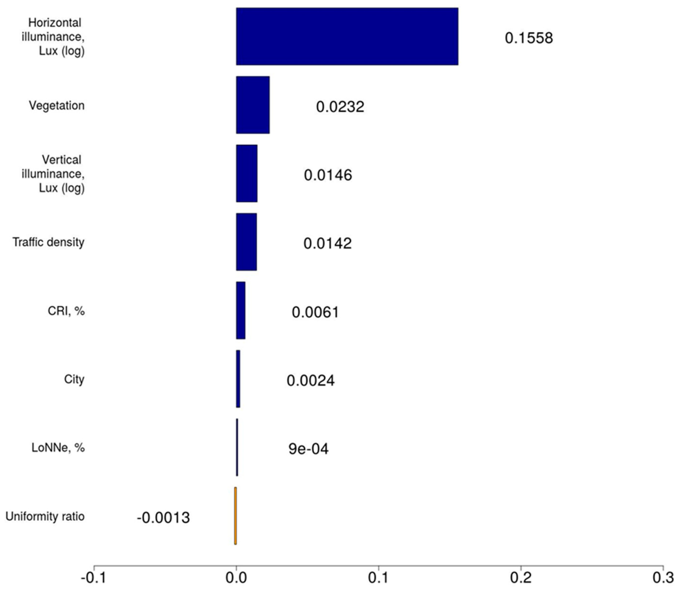
Table 2 reports three regression models, estimated for PLQI as dependent variable, while Figure 1 reports variables significantly affecting PLQI and listed in order of diminishing contribution to the model (in terms of R2-change). In particular, Model 1 in Table 2 contains SL attributes only, while Model 2 reports both SL attributes and contextual variables, and Model 3 features statistically significant PLQI predictors only.
As the models reported in Table 2 show, illuminance, both horizontal and vertical, have significant positive effects on PLQI (p < 0.01), i.e., higher values of illumination result in higher PLQI. Other factors significantly affecting PLQI are: CRI (+) (p < 0.05), vegetation (−) and traffic density (+) (p < 0.01). This means that luminaries that reveal more reliably the true colors of objects, improve PLQI. Light obscuring vegetation, quite expectedly, reduces PLQI, while higher traffic density increases it, apparently due to more dynamic lights associated with thoroughfare traffic. Characteristically, no other locational factors emerged in the models as statistically significant at the 0.05 level, thus indicating that factors significantly affecting PLQI are generally invariant across the cities under study.
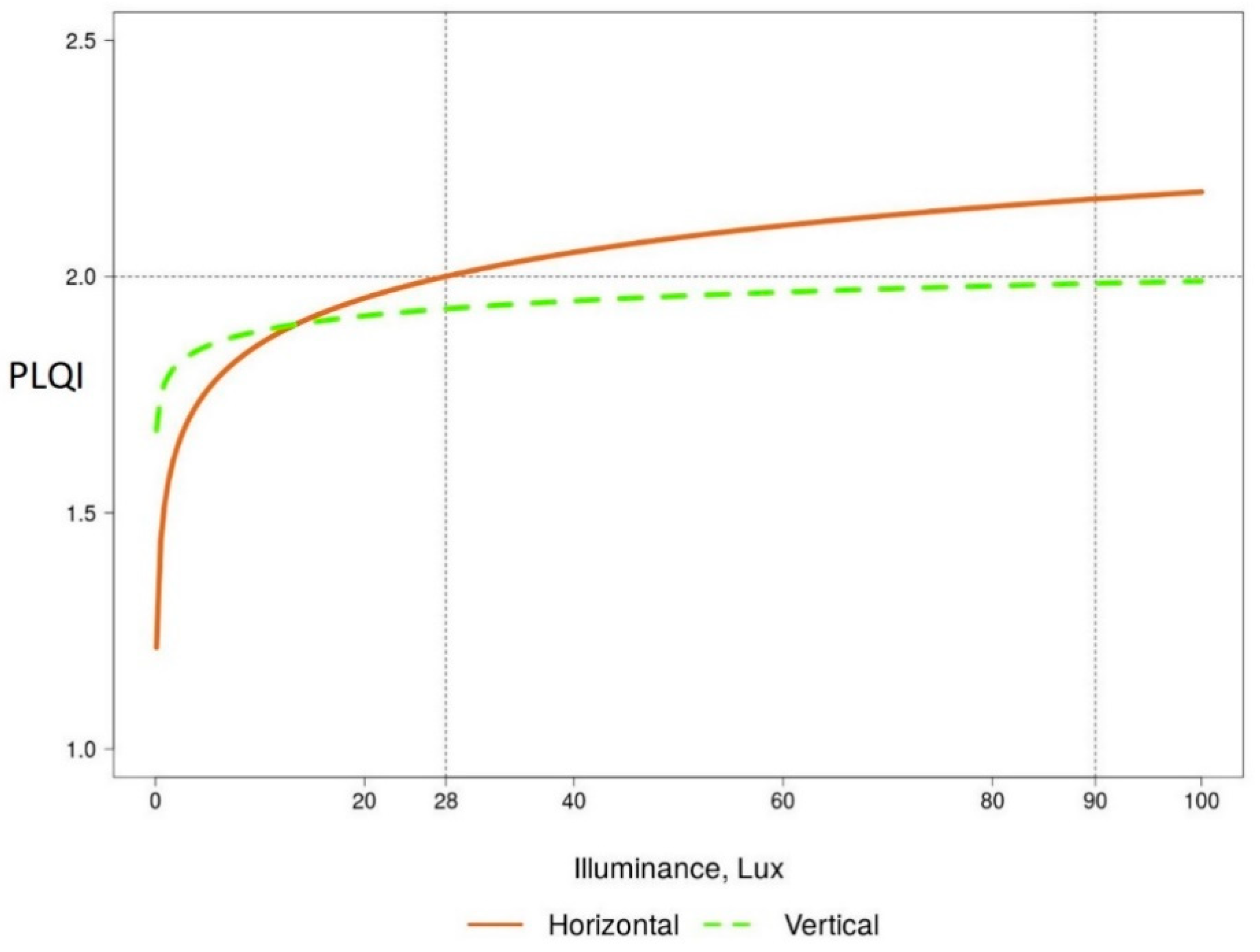
4.2. Estimating PLQI Response to Plausible Changes in Illuminance
Figure 2 demonstrates changes in PLQI in response to adjusting horizontal and vertical illuminance, which emerged as two main PLQI predictors (see Figure 1).
The response curves in Figure 2 are estimated by Model 3 (Table 2) using the following settings: the horizontal and vertical illumination levels are allowed to vary in a plausible range between 0 and 100 lx; CRI is set to its median value observed in the study area (44%); the traffic volume is set to 1 (medium traffic), and vegetation is set to 0 (no light obscuring vegetation). For the estimation, the value of vertical illumination is set to its median value, when PLQI response to plausible changes in horizontal illumination is estimated, and to the median value of horizontal illumination, when the response of vertical illumination is estimated.
As Figure 2 shows, PLQI increases monotonically with illumination, either horizontal or vertical, but from a certain point on (approximately above 28 lx), no further substantial increase in PLQI is observed, thus showing diminishing marginal returns to illumination levels above that threshold.
4.3. Model Validation
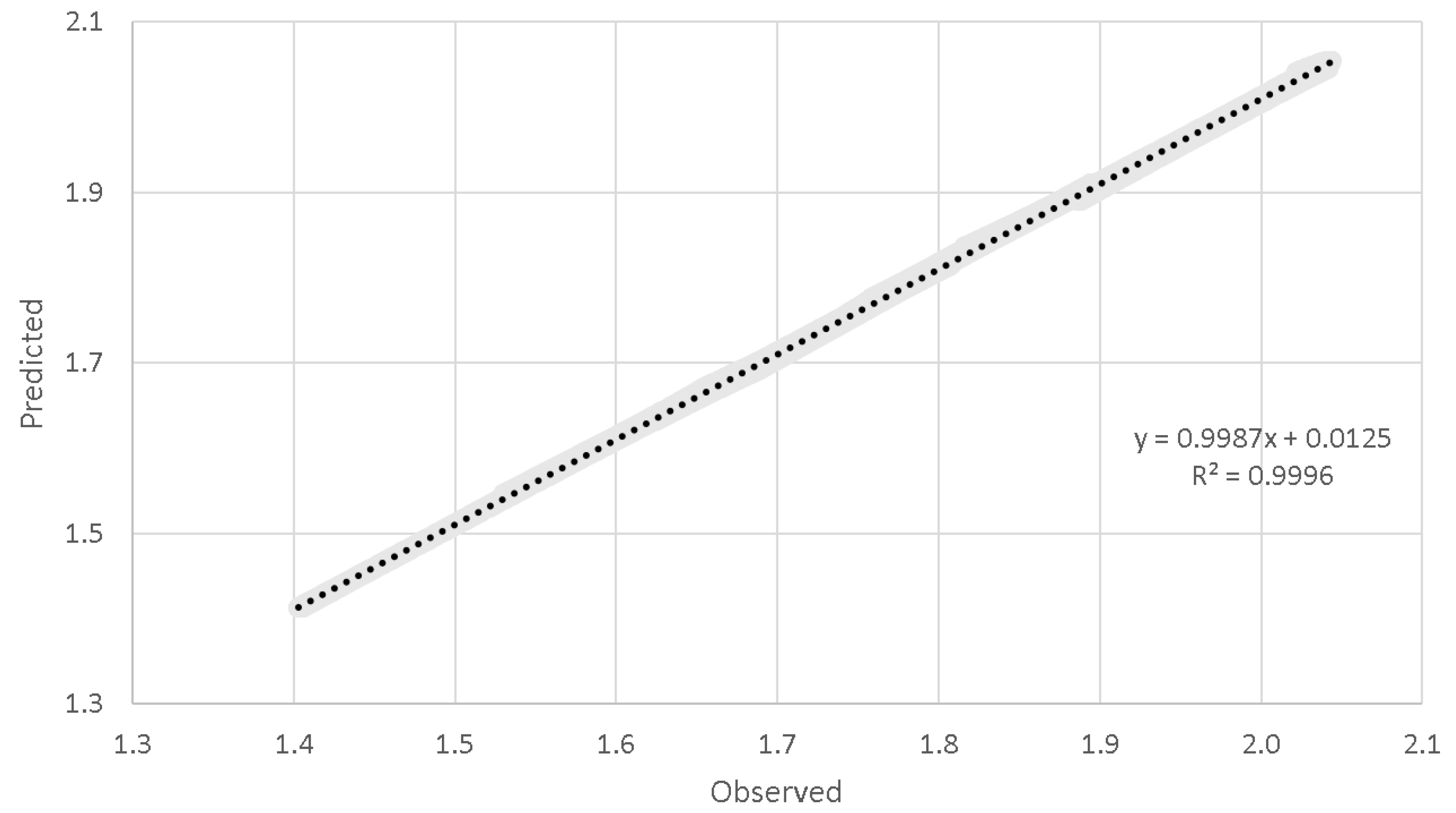
To validate the model, on which scenario assessments are to be made, and demonstrate its performance, we model-estimated PLQI values for the entire neighborhood and compared them with the PLQI values actually observed. In running the test, the values of all the input variables were set to their average values, actually observed in the study area (see Table 1), and to these values Model 3 (Table 2) was applied, to calculate PLQI estimates. Figure 3 and Figure 4 report results of this test, showing that the observed and predicted values of PLQI are highly correlated, with R2 exceeding 0.99 (see Figure 4) and exhibit nearly identical spatial patterns (see Figure 3).
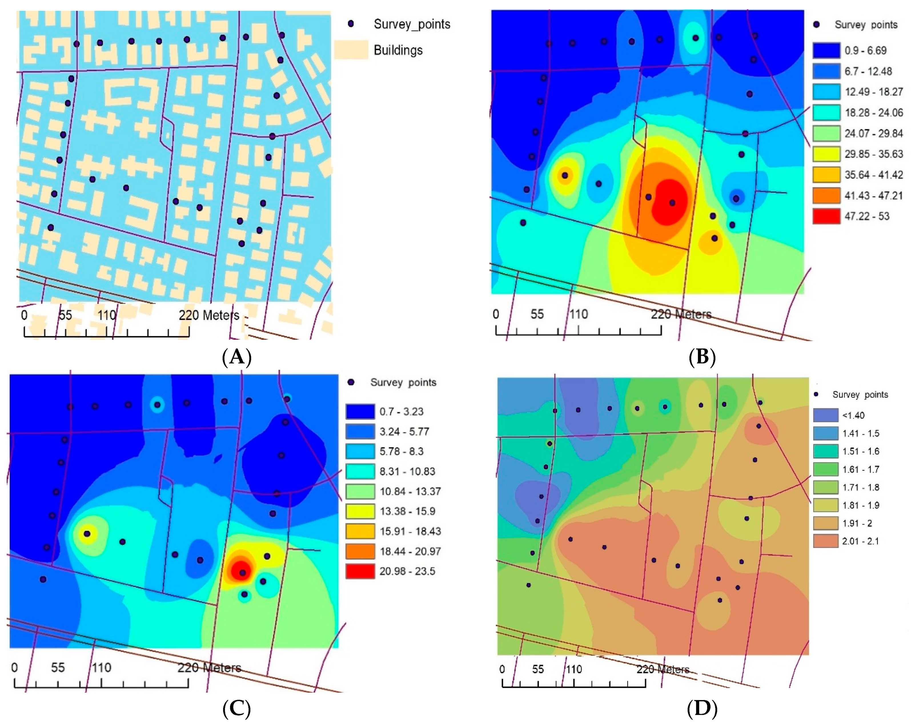
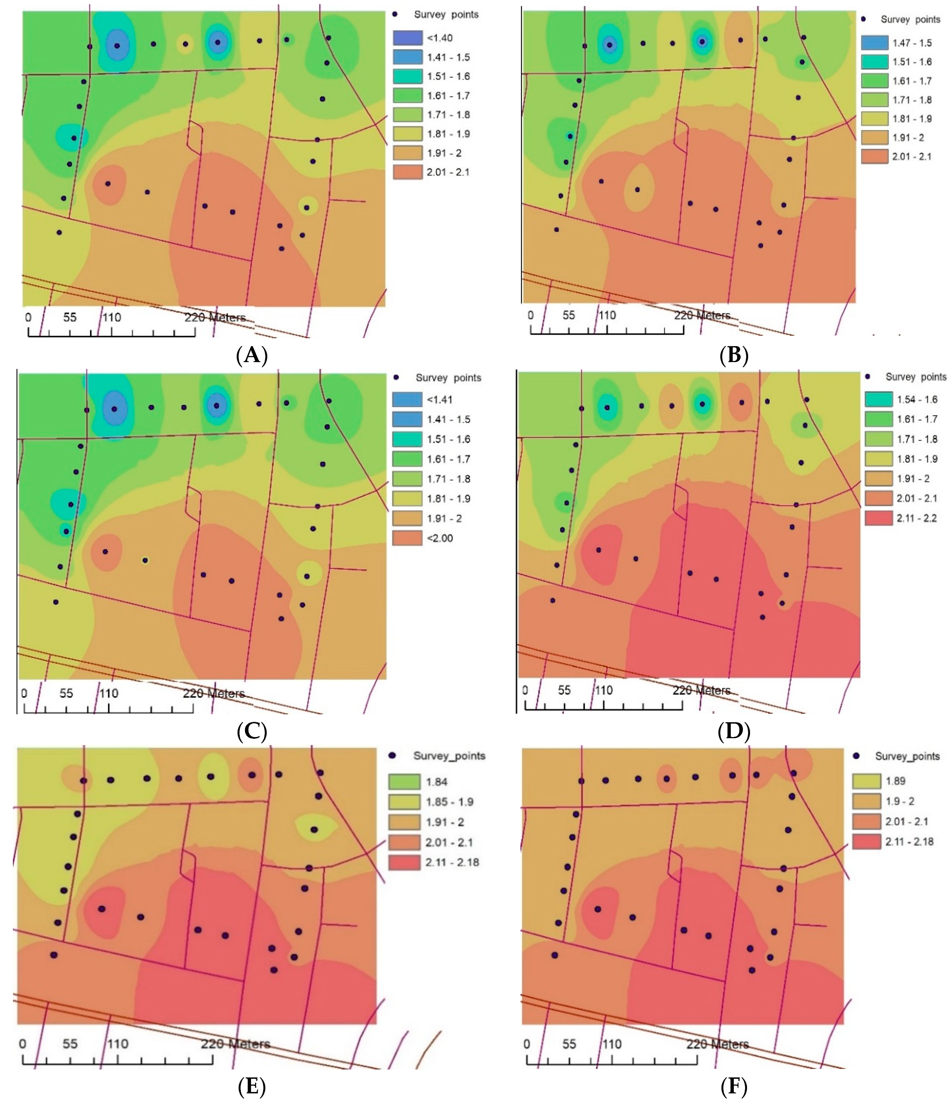
Figure 5 features several maps of the study area showing roads and buildings; instrumentally measured horizontal illuminance in lx; instrumentally measured vertical illuminance in lx, and overall SL quality assessments by the observers (PLQI). All four maps are generated by the ArcGISv10.x software (see Section 3.3), using instrumental measurements and IDW interpolations, wherever relevant. Concurrently, Figure 6 reports results of Model 3’s response tests to six different SL-adjustment scenarios:
- Reducing traffic and light-obscuring vegetation (Scenario 1, Figure 6A);
- Reducing light-obscuring vegetation and preserving a moderate traffic flow (Scenario 2, Figure 6B);
- Preserving a moderate traffic flow and keeping light-obscuring vegetation (Scenario 3, Figure 6C);
- Reducing light-obscuring vegetation and increasing traffic flow (Scenario 4, Figure 6D);
- Reducing light-obscuring vegetation and increasing traffic flow, while setting the minimum illuminance to 10 lx at each location (Scenario 5, Figure 6E), and, lastly,
- Reducing light-obscuring vegetation and increasing traffic flow, while setting the minimum illuminance to 15 lx at each location (Scenario 6, Figure 6F).
4.4. Scenario Assessment
As Figure 6 shows, the values of PLQI increase area-wide in line with increasing traffic intensity and reducing light-obscuring vegetation. Concurrently, setting illumination to at least 10 lx makes it possible to achieve the PLQI level of 1.8+ everywhere in the neighborhood (see Figure 6E,F), which almost reaches the “quite comfortable” category on the four-point PLQI assessment scale (from 0 to 3).
4.5. Energy-Saving Estimates
Horizontal illumination needed to reach PLQI of 1.8, estimated using Model 3 (Table 2), is 11.76 lx (see Section 3.5 for more details on the estimation procedure). As the levels of illumination above this value can be considered excessive, we compared this estimate to pixel-wise interpolates of instrumental measurements (see Figure 3B), and determined that about 63% of the neighborhood’s area is illuminated above this threshold. The average level of horizontal illumination in this “over-illuminated” area is 25.25 lx, i.e., more than double the needed amount of illumination. Therefore, we can conclude that reduction in the level of illumination in this “over-illuminated” area to the actually required illuminance of 11.76 lx can result in about 53.4% of energy savings ((25.25 − 11.76)/25.25 = 0.534) on SL, while keeping PLQI at 1.8 (i.e., quite comfortable) or more.
According to Tel Aviv-Yafo Municipality [19], the population of the study neighborhood is 13,410 residents, while the amount of energy spent on each resident of Tel Aviv-Yafo on SL is 176 kWh [19]. Coupled with the above-mentioned estimates of energy savings, potentially resulting from reduction in excessive street illumination, the overall energy savings in the neighborhood can be estimated as follows: 13,410 × 176 × 0.63 (63% of the neighborhood) × 0.534 (53.4% of energy savings) = 794,005 kWh, and magnitudes more in the entire metropolitan area.
5. Discussion
In this study, we suggest a novel scenario-based assessment model that can be used by urban planners and SL designers to predict the expected comfort of SL as it would be perceived by potential users. The model is based on the following five variables as inputs: instrumentally measured (or designed) horizontal and vertical illumination, CRI, presence of light obscuring vegetation, and traffic density. The model produces a PLQI metric as its output, which values range from 0 (dissatisfaction) to 3 (full satisfaction).
As the study shows, five factors emerged as main PLQI predictors: illuminance (horizontal and vertical) (p < 0.01), CRI (p < 0.05) and traffic density (p < 0.01), all of which have a statistically significant and positive effect on PLQI, while light-obscuring vegetation has a significantly negative effect on this index (p < 0.01). Characteristically, no locational factors emerged in the models as statistically significant at the 0.05 level, thus indicating that factors significantly affecting PLQI are generally invariant across different cities.
Recent studies (e.g., [20,21,22]) mention several other factors that can influence the perceived brightness of illumination, such as spatial distribution of light and surface reflectance properties. However, the effect of these factors on human perceptions was examined to date in laboratory conditions, involving only a handful number of participants.
To the best of our knowledge, the study is the first attempt to model the factors affecting PLQI in outdoor settings, while internalizing SL and controlling for environmental and contextual factors. The model’s utility is tested using a selected case study of a densely populated residential neighborhood in the City of Tel Aviv-Yafo in Israel. This test demonstrates the model’s ability to estimate PLQI’s response to changes in several contextual factors and SL attributes.
The results of the study are generally in line with the results of several previous studies [1,8,9], which indicate that human perceptions of SL are positively affected by the actual levels of illumination. However, our results seem to contradict the findings reported by Johansson et al. [9] and by Peña-García et al. [8], which identify cooler lights as contributing positively to the perception of safety and well-being in urban areas. Although we tested several light-color related metrics in our model (including CRI, CCT and LoNNe), only CRI, reflecting the ability of a light source to reliably reveal the true colors of objects, emerged statistically significant. We attribute this difference in findings to the fact that CRI and other light color-related metrics, such as CCT and LoNNe, are, in fact, collinear, although their relationship is not necessarily linear (see Appendix A Figure A1A,B). Moreover, in this study we use 254 different assessment points, aggregating 25,662 reports from individual surveyors, whereas the studies by Johansson et al. [9] and by Peña-García et al. [8] account for only ten and five assessment points, respectively.
Unlike previous studies (see inter alia [1,11,12]), this study focuses on the perceived lighting quality (PLQI), whereas previous papers modeled the feeling of safety (FoS). These are two different variables assessed separately by the surveyors. Most importantly, the study by Saad et al. [12] focuses on the overall energy savings, which can potentially be achieved by a proper selection of light color temperature and uniformity. Concurrently, in this study, we focus on the identification of over-illuminated and under-illuminated areas in a neighborhood and calculating potential energy savings that can be achieved in the former. Last, but not least, the present paper suggests a heuristic modelling procedure for assessing residents’ satisfaction with nighttime illumination, which has not been developed and empirically tested in any previous study carried out to date.
It should be emphasized, however, that our analysis does not indicate that pedestrians’ satisfaction with SL differs significantly by city, which contradicts the results previously reported in [1,11]. We explain this difference by the fact that the above studies focused on the feeling of safety (FoS) provided by SL, while this study focuses on the overall perception of SL comfort. Although these two perspectives on SL may respond similarly to some SL attributes and environmental factors (such as, e.g., illuminance, light obscuring vegetation, and traffic intensity), FoS may be stronger affected by additional environmental factors, such as local crime rates, building morphology, presence of potential escape routes, etc.
As the urban environment is a complex phenomenon, the “one-size-fits-all” principle does not always apply to different settings [1]. Therefore, using the proposed PLQI model, while internalizing the SL and environmental factors, can provide urban planners and SL designers with a valuable tool for estimating the effectiveness of their designs prior to implementation. In particular, using the proposed model can lead to altering initial SL designs, if the predicted outputs do not fully comply with predefined design objectives. Consequently, suboptimal decisions on SL can be avoided. We are unaware of any existing similar approach for assessing SL attributes, available in the empirical literature at present.
As noted in the introduction, instrumentally measured SL attributes cannot always reflect the exact feeling of comfort as that perceived by human observers. Realizing this limitation should lead to the development of instruments for integrating human assessments into the SL planning process. More specifically, future studies should determine how PLQI responds to human assessments of individual SL attributes, rather than to instrumental measurements.
Another limitation of the present research is that the utility of the proposed model was tested using only one case study. Therefore, further studies, to be carried out elsewhere, are needed to validate the model and its practical efficacy. Although our analysis demonstrates no significant differences in the factors affecting PLQI assessments across different cities, future studies should attempt to determine whether there are other affecting factors which might be significantly associated with SL perceptions.
It should also be noted that the present analysis is based on 25,662 assessment reports of SL quality averaged over some 254 assessment points. Clearly, such an aggregation entails a decrease in the efficiency of the estimated parameter due to averaging. Therefore, future studies should attempt to look at the potential effects of individual factors, such age, gender, personality, etc., on SL perceptions, employing, to this end, different modelling approaches, such as ordinal and generalized ordinal regressions.
Lastly, we should remark that the CRI index, employed in the study, is widely accepted and commonly used illumination metric by lighting producers and measurement equipment manufacturers, as well as by policy-makers [23]. The index in question was developed by the International Commission on Illumination (CIE) in the 1960s and is commonly termed the “CIE assessment method” [24]. However, in recent studies, the method is criticized for inability to predict the full range of perceived color aspects, with alternative fidelity assessment methods, based on differences in a large variety of colors, being proposed [23,24,25]. Further studies may consider these alternative metrics, providing that measurement equipment required is available to researchers.
6. Conclusions
The empirical approach, developed and tested in this study, can provide urban planners and SL designers with a valuable tool for ensuring the comfort of urban residents after dark. Such a tool is oriented to assure maximum efficiency of energy usage related to SL. In particular, the PLQI model estimated in this study, as well as the proposed way of its integration into scenario-assessment process, can assist decision makers in estimating the perceived comfort of SL systems prior to installation, instead of relying solely on universal lighting standards, which are mainly geared to motor traffic [14]. Implementing such an approach may significantly increase the satisfaction of pedestrians, who form a major share of street users.
An important feature of the proposed PLQI model is that it uses a limited number of relatively easy-to-estimate inputs, routinely calculated by SL designers. These include, inter alia, horizontal and vertical illumination and CRI, as well as several contextual variables, such presence of light obscuring vegetation and traffic density. The model’s outputs are also relatively easy to interpret, as the PLQI’s values range from 0 (dissatisfaction) to 3 (full satisfaction). However, no specific technical parameters of the lighting installations (such as type of luminaries, spatial distribution of lamps, etc.), needed to achieve the required illumination settings, have been estimated by the study, providing that such parameters can be determined ad hoc by lighting engineers.
Lastly, we should note that the model developed in this study helps to determine potential energy savings associated with reduction of excessive SL, which we estimated in our case study to reach about 50%. Considering well-established negative impacts of artificial illumination on the ecosystem health [26], such a reduction in excessive SL can have important ecosystem benefits and thus contribute to sustainable development goals. However, further studies, to be carried out elsewhere, may be needed to determine the generality of our findings.
Author Contributions
Conceptualization, B.A.P.; formal analysis, R.S.; methodology, B.A.P.; writing—original draft, B.A.P. and R.S.; funding acquisition, B.A.P. and T.T. All authors have read and agreed to the published version of the manuscript.
Funding
Israel Ministry of Science & Technology (under Grant number 35740).
Institutional Review Board Statement
Approved by the University of Haifa Ethics Committee (Approval # 177/19).
Informed Consent Statement
All the survey participants filled in an online informed consent form, prior to their participation in the survey.
Data Availability Statement
The data are property of the funding institution and may be requested via a proper data request procedure.
Acknowledgments
The authors are grateful to Dialog Ltd., Inna Nissenbaum and Alina Svechkina for helping to assemble data for this research.
Conflicts of Interest
The authors declare no conflict of interest.
Appendix A

Table A1.
Frequency statistics of selected research variables (total number of individual reports = 25,662; total number of SL assessment points = 254).
Table A1.
Frequency statistics of selected research variables (total number of individual reports = 25,662; total number of SL assessment points = 254).
| Variable | Observation Count | Percent |
|---|---|---|
| Assessment points | ||
| 106 | 41.73 |
| 73 | 28.74 |
| 75 | 29.53 |
| Total: | 254 | 100.00 |
| Number of observers | ||
| 165 | 41.67 |
| 133 | 33.58 |
| 98 | 24.75 |
| Total: | 396 a | 100.00 |
| Vegetation density | ||
| 120 | 47.24 |
| 104 | 40.94 |
| 30 | 11.82 |
| Total: | 254 | 100.00 |
| Traffic intensity | ||
| 146 | 57.48 |
| 81 | 31.89 |
| 27 | 10.63 |
| Total: | 254 | 100.00 |
a Altogether, 380 people participated in the study, however 16 of them performed assessments in more than one city. Therefore, the exhibited total number is 396.
Figure A1.
Scatterplots showing the relationships between illumination indices—(A) CRI vs. CCT; and (B) CRI vs. LoNNe.
Figure A1.
Scatterplots showing the relationships between illumination indices—(A) CRI vs. CCT; and (B) CRI vs. LoNNe.

References
- Svechkina, A.; Trop, T.; Portnov, B.A. How much lighting is required to feel safe when walking through the streets at night? Sustainability 2020, 12, 3133. [Google Scholar] [CrossRef] [Green Version]
- Johansson, M.; Rosén, M.; Küller, R. Individual factors influencing the assessment of the outdoor lighting of an urban footpath. Lighting Res. Technol. 2011, 43. [Google Scholar] [CrossRef]
- Wu, S. Investigating Lighting Quality: Examining the Relationship between Pedestrian Lighting environment and perceived Safety. Blackburg. Virginia 2014. Available online: https://vtechworks.lib.vt.edu/handle/10919/48170 (accessed on 9 January 2021).
- European Standards. EN 13201-1-5-Road Lighting. EN 13201, Road lighting—Part 2: Performance Requirements. 2015. Available online: https://www.en-standard.eu/csn-en-13201-1-4-road-lighting/ (accessed on 6 May 2020).
- IES. RP-8-14: Roadway Lighting (ANSI Approved), Illuminating Eng.; Illuminating Engineering Society: Wall Street, NY, USA, 2014. [Google Scholar]
- Boyce, P.R.; Eklund, N.H.; Hamilton, B.J.; Bruno, L.D. Perceptions of safety at night in different lighting conditions. Lighting Res. Technol. 2000, 32, 79–91. [Google Scholar] [CrossRef]
- Kaparias, I.; Bell, M.G.H.; Miri, A.; Chan, C.; Mount, B. Analysing the perceptions of pedestrians and drivers to shared space. Transp. Res. Part F Traffic Psychol. Behav. 2012, 15, 297–310. [Google Scholar] [CrossRef]
- Peña-García, A.; Hurtado, A.; Aguilar-Luzón, M.C. Impact of public lighting on pedestrians’ perception of safety and well-being. Saf. Sci. 2015, 78, 142–148. [Google Scholar] [CrossRef]
- Johansson, M.; Pedersen, E.; Maleetipwan-Mattsson, P.; Kuhn, L.; Laike, T. Perceived outdoor lighting quality (POLQ): A lighting assessment tool. J. Environ. Psychol. 2014, 39. [Google Scholar] [CrossRef]
- Park, Y.; Garcia, M. Pedestrian safety perception and urban street settings. Int. J. Sustain. Transp. 2020, 14, 860–871. [Google Scholar] [CrossRef]
- Portnov, B.A.; Saad, R.; Trop, T.; Kliger, D.; Svechkina, A. Linking nighttime outdoor lighting attributes to pedestrians’ feeling of safety: An interactive survey approach. PLoS ONE 2020, 15, e0242172. [Google Scholar] [CrossRef]
- Saad, R.; Portnov, B.A.; Trop, T. Saving energy while maintaining the feeling of safety associated with urban street lighting. Clean Technol. Environ. Policy 2020. [Google Scholar] [CrossRef]
- Rahm, J.; Johansson, M. Assessing the pedestrian response to urban outdoor lighting: A full-scale laboratory study. PLoS ONE 2018, 13, e0204638. [Google Scholar] [CrossRef] [PubMed] [Green Version]
- Patching, G.R.; Rahm, J.; Jansson, M.; Johansson, M. A New Method of Random Environmental Walking for Assessing Behavioral Preferences for Different Lighting Applications. Front. Psychol. 2017, 8, 345. [Google Scholar] [CrossRef] [PubMed] [Green Version]
- Laudon, K.C.; Laudon, J.P. Management Information Systems: Managing the Digital Firm, Global Edition, 15th ed.; Pearson: London, UK, 2018. [Google Scholar]
- Maleetipwan-Mattsson, P.; Laike, T.; Johansson, M. Self-Report Diary: A Method to Measure Use of Office Lighting. Leukos 2013, 9, 291–306. [Google Scholar] [CrossRef]
- LoNNe. Protected areas in Europe: Essential for safeguarding the nighttime environment. In the Statement of the EU-COST Action ES 1204: Cost-LoNNe; LoNNe: Berlin, Germany, 2016. [Google Scholar]
- ArcGIS–ESRI. ArcGIS Desktop 10.7.1 Quick Start Guide. Available online: https://desktop.arcgis.com/en/quick-start-guides/10.7/arcgis-desktop-quick-start-guide.htm (accessed on 15 August 2020).
- Tel Aviv-Yafo Municipality. 2020. Available online: https://www.tel-aviv.gov.il/Transparency/Pages/Quarter.aspx (accessed on 2 December 2020).
- Hwang, T.; Tai, J. Effects of Indoor Lighting on Occupants’ Visual Comfort and Eye Health in a Green Building. Indoor Built Environ. 2011, 20, 75–90. [Google Scholar] [CrossRef]
- Duff, J.; Kelly, K.; Cuttle, C. Spatial brightness, horizontal illuminance and mean room surface exitance in a lighting booth. Lighting Res. Technol. 2017, 49, 5–15. [Google Scholar] [CrossRef] [Green Version]
- Durmus, D.; Davis, W. Blur perception and visual clarity in light projection systems. Opt. Express 2019, 27, A216–A223. [Google Scholar] [CrossRef] [PubMed]
- Davis, W.; Ohno, Y. Approaches to color rendering measurement. J. Mod. Opt. 2009, 56, 1412–1419. [Google Scholar] [CrossRef]
- Wei, M.; Royer, M.; Huang, H.-P. Perceived colour fidelity under LEDs with similar Rf but different Ra. Lighting Res. Technol. 2019, 51, 858–869. [Google Scholar] [CrossRef]
- Sándor, N.; Schanda, J. Visual colour rendering based on colour difference evaluations. Lighting Res. Technol. 2006, 38, 225–239. [Google Scholar] [CrossRef]
- Svechkina, A.; Portnov, B.A.; Trop, T. The impact of artificial light at night on human and ecosystem health: A systematic literature review. Landsc. Ecol. 2020. [Google Scholar] [CrossRef]
Figure 1.
Ranking of the factors found to affect PLQI. (Note: The factors are ranked in descending order according to changes in ΔR2; see Table 2 and text for explanations).
Figure 1.
Ranking of the factors found to affect PLQI. (Note: The factors are ranked in descending order according to changes in ΔR2; see Table 2 and text for explanations).

Figure 2.
Model-response test of PLQI to plausible changes in horizontal and vertical illuminance (see text for explanations). Notes: Model 3 in Table 2 is used for estimates; the illuminance values are allowed to vary, while CRI is set to its median value (44%), traffic volume is set to 1 (medium traffic) and light-obscuring vegetation is set to zero (no light-obscuring vegetation).

Figure 3.
Observed (A) vs. predicted (B) values of PLQI in the study neighborhood (Note: The predictions are based on Model 3 (Table 2), applied to individual pixels of the neighborhood map (see Figure 3).

Figure 4.
Correspondence between the observed and predicted values of PLQI in the study neighborhood. Note: See Footnote to Figure 5
Figure 4.
Correspondence between the observed and predicted values of PLQI in the study neighborhood. Note: See Footnote to Figure 5

Figure 5.
Maps of the study area showing roads and buildings (A); instrumentally measured horizontal illuminance levels in lx (B); instrumentally measured vertical illuminance in lx (C); and PLQI assessments by the observers (D). Notes: Maps (B–D) are produced using the inverse distance weighted (IDW) interpolation method.

Figure 6.
Estimated PLQI response to plausible changes in different input variables (see text for explanations). (A) Traffic = 0 & Vegetation = 0; (B) Traffic = 1 & Vegetation = 0; (C) Traffic = 1 & Vegetation = 1; (D) Traffic = 2 & Vegetation = 0; (E) Traffic = 2 & Vegetation = 0, Horizontal illuminance ≥ 10 lx; (F) Traffic = 2 & Vegetation = 0, Horizontal illuminance ≥ 15 lx; Notes: The estimates are based on Model 3 (Table 2); the maps are produced using the IDW interpolation method.

Table 1.
Descriptive statistics of the research variables.
| Variable | Number of Valid Measurements | % | Median | Mean | SD | Min | Max |
|---|---|---|---|---|---|---|---|
| Dependent Variable | |||||||
| Perceived lighting quality index (PLQI) | 254 | - | 1.83 | 1.77 | 0.30 | 0.94 | 2.30 |
| PSL Attributes | |||||||
| Vertical illuminance, lx (ln) | 254 | - | 1.88 | 1.79 | 0.98 | −0.92 | 4.00 |
| Horizontal illuminance, lx (ln) | 254 | - | 2.36 | 2.19 | 1.16 | −1.66 | 4.36 |
| Color rendering index (CRI) | 254 | - | 44 | 48 | 25 | 1 | 93 |
| LoNNe index, % | 254 | - | 8.50 | 10.50 | 6.26 | 2.90 | 30.00 |
| Correlated color temperature (CCT), Kelvins | 254 | - | 2262 | 2730 | 919 | 1688 | 5878 |
| Uniformity ratio | 254 | - | 0.57 | 0.55 | 0.21 | 0.03 | 0.94 |
| Locational Factors | |||||||
| City dummies: | |||||||
| 106 | 41.73 | - | - | - | - | - |
| 73 | 28.74 | - | - | - | - | - |
| 75 | 29.53 | - | - | - | - | - |
| Environmental Factors | |||||||
| Traffic density | 254 | - | 0.00 | 0.53 | 0.68 | 0.00 | 2.00 |
| Vegetation | 254 | - | 1.00 | 0.65 | 0.68 | 0.00 | 2.00 |
Table 2.
Factors affecting PLQI in the study cities (Method—ordinary least square (OLS) regression).
Table 2.
Factors affecting PLQI in the study cities (Method—ordinary least square (OLS) regression).
| Variable | Model 1 | Model 2 | Model 3 | |||
|---|---|---|---|---|---|---|
| B a | t-Stat b | B a | t-Stat b | B a | t-Stat b | |
| (Constant) | 1.254 | 22.834 *** | 1.363 | 23.100 *** | 1.330 | 32.212 *** |
| SL attributes: | ||||||
| Vertical illuminance, lx (log) | 0.050 | 2.834 *** | 0.051 | 2.956 *** | 0.046 | 2.708 *** |
| Horizontal illuminance, lx (log) | 0.147 | 9.802 *** | 0.134 | 9.164 *** | 0.140 | 9.669 *** |
| CRI, % | 0.002 | 2.480 ** | 0.002 | 2.057 ** | 0.001 | 2.527 ** |
| LoNNe, % | −0.003 | −1.065 | −0.004 | −1.216 | - | - |
| Uniformity ratio | 0.079 | 1.238 | 0.034 | 0.545 | - | - |
| Locational Attributes: | ||||||
| City dummies (ref. = Tel Aviv) | ||||||
| - | - | −0.002 | −0.044 | - | - |
| - | - | −0.058 | −1.728 * | - | - |
| Environmental Attributes: | ||||||
| - | - | 0.059 | 2.925 *** | 0.064 | 3.312 *** |
| - | - | −0.072 | −3.655 *** | −0.070 | −3.689 *** |
| Number of observations | 254 | 254 | 254 | |||
| R2 | 0.50 | 0.56 | 0.55 | |||
| R2- adjusted | 0.49 | 0.54 | 0.54 | |||
| F-statistic | 50.55 *** | 34.01 *** | 60.19 *** | |||
Notes: *** indicates a 1% significance level (two-tailed); ** indicates a 5% significance level (two-tailed); * indicates a 10% significance level (two-tailed); a unstandardized regression coefficient; b t-statistic and its significance level. Model 1: Model with PSL attributes variables only; Model 2: Augmented model with all explanatory variables included; Model 3: Model with significant variables only.
Publisher’s Note: MDPI stays neutral with regard to jurisdictional claims in published maps and institutional affiliations. |
© 2021 by the authors. Licensee MDPI, Basel, Switzerland. This article is an open access article distributed under the terms and conditions of the Creative Commons Attribution (CC BY) license (http://creativecommons.org/licenses/by/4.0/).
Share and Cite
MDPI and ACS Style
Portnov, B.A.; Saad, R.; Trop, T. Interactive Scenario-Based Assessment Approach of Urban Street Lighting and Its Application to Estimating Energy Saving Benefits. Energies 2021, 14, 378. https://doi.org/10.3390/en14020378
AMA Style
Portnov BA, Saad R, Trop T. Interactive Scenario-Based Assessment Approach of Urban Street Lighting and Its Application to Estimating Energy Saving Benefits. Energies. 2021; 14(2):378. https://doi.org/10.3390/en14020378
Chicago/Turabian StylePortnov, Boris A., Rami Saad, and Tamar Trop. 2021. "Interactive Scenario-Based Assessment Approach of Urban Street Lighting and Its Application to Estimating Energy Saving Benefits" Energies 14, no. 2: 378. https://doi.org/10.3390/en14020378
Note that from the first issue of 2016, this journal uses article numbers instead of page numbers. See further details here.