Interannual Variation in Night-Time Light Radiance Predicts Changes in National Electricity Consumption Conditional on Income-Level and Region


1
Fondazione Eni Enrico Mattei, Corso Magenta 63, 20123 Milano, Italy
2
Catholic University of Milan, Largo Gemelli 1, 20123 Milan, Italy
*
Author to whom correspondence should be addressed.
Energies 2019, 12(3), 456; https://doi.org/10.3390/en12030456
Submission received: 27 December 2018
/
Revised: 29 January 2019
/
Accepted: 30 January 2019
/
Published: 31 January 2019
(This article belongs to the Special Issue Data Analytics in Energy Systems)
Abstract
:Using remotely-sensed Suomi National Polar-orbiting Partnership (NPP)-VIIRS (Visible Infrared Imagery Radiometer Suite) night-time light (NTL) imagery between 2012 and 2016 and electricity consumption data from the IEA World Energy Balance database, we assemble a five-year panel dataset to evaluate if and to what extent NTL data are able to capture interannual changes in electricity consumption within different countries worldwide. We analyze the strength of the relationship both across World Bank income categories and between regional clusters, and we evaluate the heterogeneity of the link for different sectors of consumption. Our results show that interannual variation in nighttime light radiance is an effective proxy for predicting within-country changes in power consumption across all sectors, but only in lower-middle income countries. The result is robust to different econometric specifications. We discuss the key reasons behind this finding. The regions of Sub-Saharan Africa, Middle-East and North Africa, Latin America and the Caribbeans, and East Asia and the Pacific render a significant outcome, while changes in Europe, North America and South Asia are not successfully predicted by NTL. The designed methodological steps to process the raw data and the findings of the analysis improve the design and application of predictive models for electricity consumption based on NTL at different spatio-temporal scales.
1. Introduction
Over the last 20 years, the release of open-access night-time light (NTL) data with worldwide coverage has proven useful for estimating multiple aspects of human development at both a global [1] and a local scale [2]. Different generations of data have been published by National Aeronautics and Space Administration (NASA) and National Oceanic and Atmospheric Administration (NOAA) (including the Defence Meteorological Satellite Program-Operational Linescan (DMSP-OLS), the Visible Infrared Imagery Radiometer Suite–day-night band (VIIRS-DNB) [3], and the upcoming Black Marble [4] products) and have been continuing to improve in data quality and increasing spatial and temporal resolutions. Extensive research has been carried out on NTL data, in a large range of applications, including as a proxy for electricity-related indicators (e.g., electricity demand [5,6,7,8,9,10], power supply reliability and outages [11,12], household electrification [13,14,15,16,17], electricity demand peaks visualisation [18]) and socio-economic development metrics (including economic growth [19], poverty detection [20], inequality [21] and greenhouse gas emissions [22]).
At the same time, a growing demand for reliable data to support decision-makers has been witnessed in recent years. The greatest roadblocks are found in the context of developing countries, where data availability is affected by a broad spectrum of issues, including the financial, technical, or infrastructure constraints to collect and maintain up-to-date data, but also data quality issues. This has been of particular relevance in the objective of tracking progress towards the United Nations’ Sustainable Development Goals. In response to such challenges, novel approaches to complement the on-the-field data collection that is resource-consuming and often subject to potential errors are gaining significance and international support (e.g., using remote sensing for measuring agricultural yield [23] or monitoring deforestation [24]).
In this paper we present a number of exploratory findings in the prospect of using and validating NTL-based tools for the monitoring of electricity consumption at different spatial and temporal scales (as already explored in a number of recent contributions [8,25,26,27]). The necessity to carry our exploratory analysis stems from a strong caveat characterizing approaches based on remotely-sensed data, namely that they should be used in parallel and not in substitution of more precise methodologies, as satellite output data may include some long-term, unaccounted-for bias which could significantly affect the results. For this reason, a continuous validation of those data is strongly suggested, so as to factor potential evolution of the energy system and data issues in the estimation model.
Specifically, we evaluate if and to which extent the increase in per-capita gross national income (GNI) leads to a significant variation of the relation NTL vs electricity consumption in its different components. Our hypothesis is that at higher levels of economic development, electricity consumption reaches a threshold where the lighting component becomes a marginal share of the Total Final Consumption. This is particualrly important given the forecasted growing importance of electricity in the global energy mix [28]. We also analyze the strength of the relationship across regional clusters. We run log-log regressions analysis, implementing pooled-OLS (ordinary least squares), country fixed-effects, and country-year demeaning specifications. This is done subsetting observations for each income category when testing the income hypothesis, and by creating interaction terms when assessing the NTL-power consumption relationship across regional clusters.
The remainder of the paper is structured as follows: In Section 2 and Section 3 we present the materials collected and methods designed and applied, respectively, including a discussion of the data and of the relative challenges which had to be tackled. Section 4 presents the log-log regression results for income-categories and regions for total final consumption (TFC) of electricity. In Section 5, the key findings and limitations of the study are discussed, and future research prospects are highlighted. The Appendix A includes regression results across further power consumption sectors and additional figures.
2. Materials
Remotely-sensed NTL data is derived from Suomi National Polar-orbiting Partnership (NPP)-VIIRS (Visible Infrared Imager Radiometer Suite) monthly composites [3]. Images have been retrieved for the period between April 2012 and December 2016. Each raster file has a resolution of 15-arc seconds, corresponding to 450 m at nadir. The data is partially pre-processed at the source, i.e., it comes with a two-step correction to be be cloud-free and lunar illuminance-free. In particular, the day-night band (DNB) sensor collects data multiple times a day, both during the day and the night, and aggregates such images in daily snapshots, which are then averaged into monthly composites at the pixel-level, and days with cloud-cover disturbances are discarded. Each pixel contains information on the mean detected radiance (expressed in µ units). As discussed in the literature [29,30,31], irrespective of corrections, the raw data is affected by a range of issues which needs to be tackled by an appropriate processing procedure. These are discussed in the Methods section.
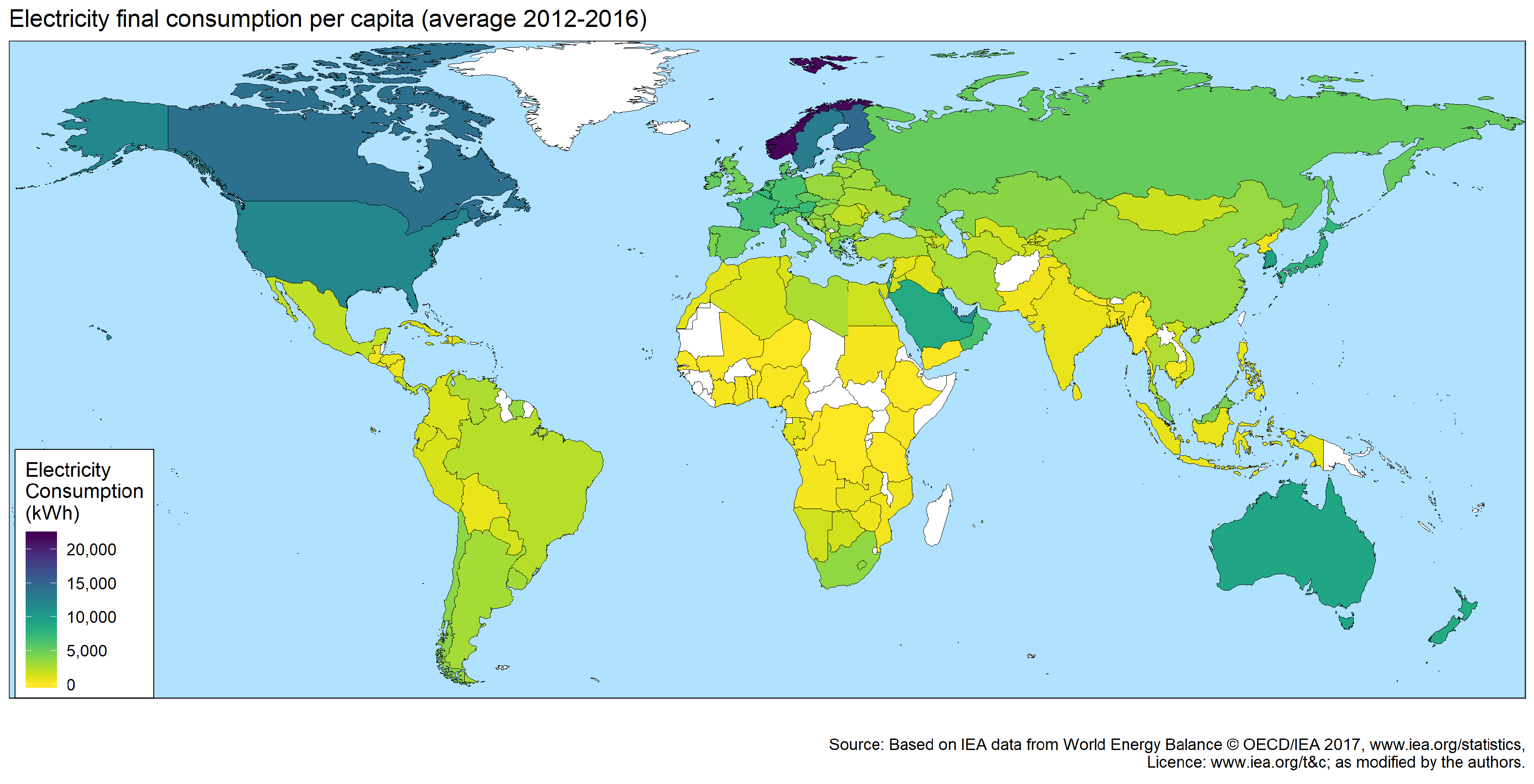
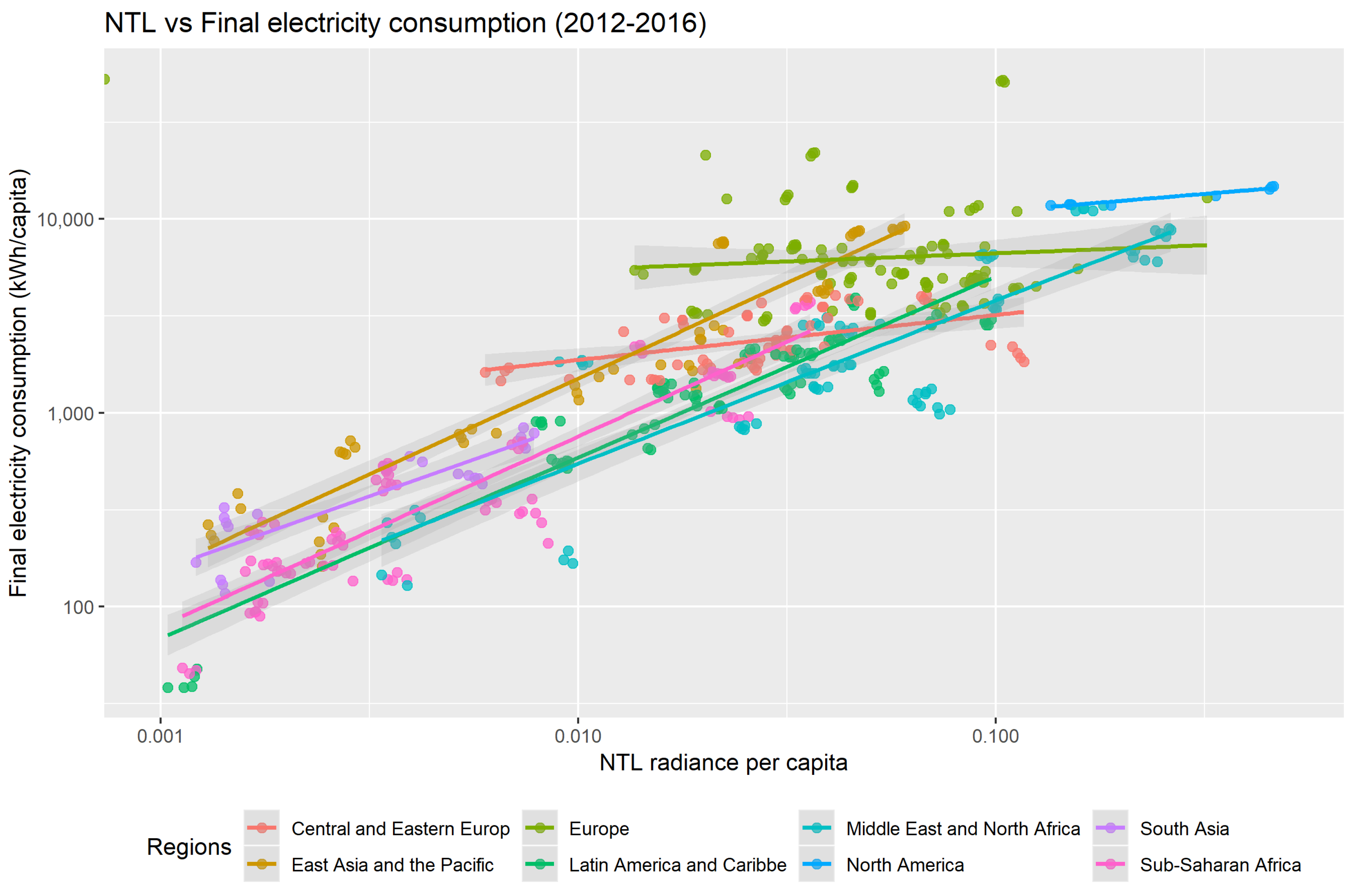
Electricity consumption data has been collected by the IEA World Energy Balance database [32], which represents the most reliable, standardized, and continuous available time series of energy data worldwide. For this study the electricity final consumption has been considered, by analyzing: (1) total final (shown in Figure 1), (2) residential and (3) commercial and public services consumption. The data is available with annual detail, and the most recent with a worldwide coverage area for the year 2016. For this reason, as they are only partially overlapping with the night-time light data, the analysis will be limited to the 2012–2016 period. Other sources provide more up-to-date information but on a limited number of countries (mainly OECD countries), and therefore they are less useful for the global scope of this research. The total number of countries considered amounts to 109, including 13 for Central and Eastern Europe, 11 in East Asia and the Pacific, 24 for Europe, 18 for Latin American and the Caribbeans, 16 for the Middle East and North Africa, two for North America, five for South Asia, and 20 for Sub-Saharan Africa). A caveat stems from the classification of the different typologies of power consumption: While the IEA aims at providing standard-quality data, there might still be differences in the accounting and categorization of power consumption between countries.
Finally, per-capita GNI (calculated with the World Bank Atlas method ( The Atlas conversion factor for any year is the average of a country’s exchange rate for that year and its exchange rates for the two preceding years, adjusted for the difference between the rate of inflation in the country and international inflation; the objective of the adjustment is to reduce any changes to the exchange rate caused by inflation. (The World Bank (2018))) is acquired for each year and each country from the World Bank Data Portal (indicator NY.GNI.PCAP.CD). Based on thresholds reported for each year [33], we create a categorical variable with income categories, resulting in low-income (on average, ), lower-middle income (), upper-middle income (), and high-income () countries clusters.
3. Methods
The NTL data processing has been implemented within the Google Earth Engine interface [34], a cloud-computing Javascript console and interface for remotely sensed data elaboration (refer to the Source code section for the repository hosting the script, which allows results reproduction, updating, and parameters alteration). As discussed in [29], due to calibration issues in each monthly tile, a number of cells contain very small, sometimes negative values (which in radiance terms do not make sense), that are identified as sensor and calibration noise, rather than actual radiance. At the same time, the radiance data is affected by the albedo of land surface (which can lead to the observed radiance abnormally fluctuating across seasons due to vegetation phenology, snow, and ice cover [18,35]). As shown in Table 1, removing pixels with very small radiance values—which cannot be identified as stable anthropogenic light—lead to very significant drops in the light metrics. This is particularly relevant in snow-covered countries. To cope with both issues, after an empirical assessment of cells values across the world, cells with radiance value < have been set to zero.
In the same fashion, disproportionately large-value pixels (of several orders of magnitude) are occasionally observed among a number of oil and gas-producing countries, mainly owing to flaring activity not being filtered out by the processing algorithm (refer to [36]). In fact, observing Landsat or Sentinel satellite imagery in the proximity of such pixels reveals the presence of extraction sites. Table 2 compares the median sum of light in top flaring producing countries (as according to data from the World Bank’s Global Gas Flaring Reduction Partnership [37]) with and without the correction adopted in this study, i.e., where we set all pixels with a radiance value to 0, and it shows how such pixels in some countries (e.g., Algeria, Nigeria, Iraq and Iran) contribute to a very large share of the total detected radiance, and thus are prone to bias the analysis. Interestingly, the same procedure does not change drastically the value in two control oil and gas producing countries where substantially less flaring is reported (United Kingdom or India).
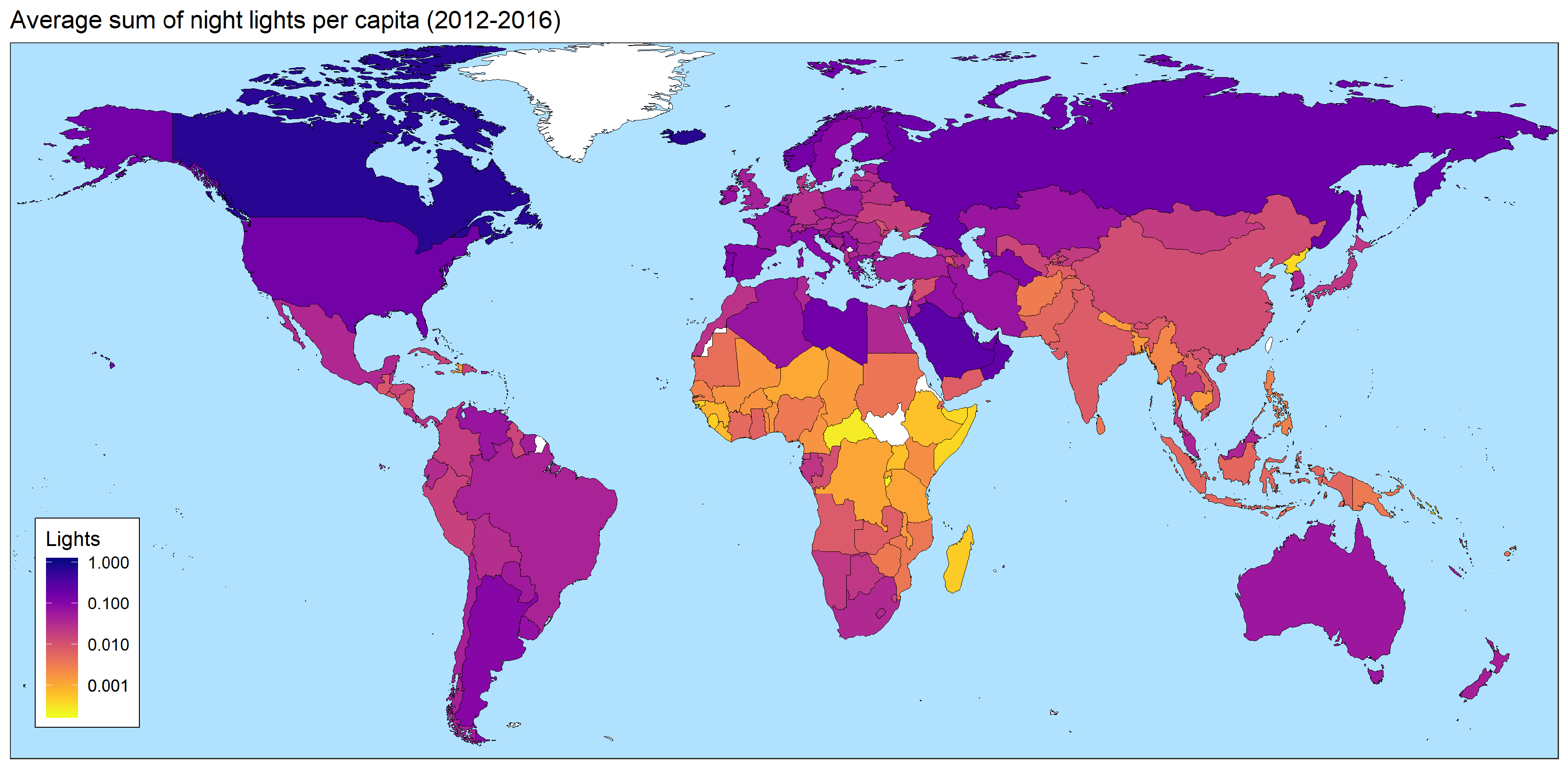
Subsequently, the raster files’ projection has been adjusted to a world cylindrical equal area (Lambert) projection (SR-ORG:8287) to enable a consistent computation, since the original file came in the standard EPSG:4326 projection, where the pixel resolution is of 450 m (the linear resolution equivalent of 15 arcseconds) at nadir but it changes as one moves away from the equator. The median annual value at each pixel has been considered, and the sum of the total radiance within each country has then been calculated for each country. The median has been favoured over the mean to discard anomalous months in terms of detected radiance. The figure has been divided by the national population, and has been defined as . The annual values of for each country are represented in Figure 2.
The yearly country-level figures have then been joined with the IEA electricity consumption database and with per-capita GNI measures. To assess the predictive power of NTL over actual consumption levels, log-log regressions have been performed using the following general specification:
where is the natural logarithm of electric consumption for the given category, is the natural logarithm of NTL, and is the corresponding estimated regression coefficient. Given the log-log specification—the regression coefficient is to be interpreted as the predicted % change in electric consumption in response to a 1% change in NTL intensity. represents the country fixed-effects (controlling for the mean level of NTL radiance in that country, allowing the regression coefficient to be interpreted as a within-estimator), are the year fixed-effects (controlling for world-wide year events e.g., particularly snowy years affecting the albedo, or to changes in the satellite calibration), is a vector of stochastic error terms, t are years, c are countries. Three comparative specifications, including only the NTL coefficient, adding country fixed-effects, and adding also year fixed-effects, have been run.
The main purpose of the analysis is investigating to which extent the yearly per-capita average radiance is capable of predicting interannual variations across different sectorial per-capita electricity consumption figures. Observations have been initially grouped into the income categories defined by The World Bank (low-income, lower-middle income, upper-middle income, and high-income economies).
The exercise has then been reiterated, but in this case the figures have been clustered by macro-region, where the world has been split into seven macro-areas, including: Central and Eastern Europe, Middle-East and North Africa, Sub-Saharan Africa, South Asia, East Asia and the Pacific, and the Americas. In this, case interaction terms between the categorical variables for each region and the log(NTL) variable have been introduced in the specification—as in Equation (2)—to assess the heterogeneity in the effect across regional clusters.
Here, is the usual coefficient measuring the main effect of the log(NTL); is a vector of coefficients representing the main effect estimators each region (regions are introduced as levels of a categorical variable, with r identifying each region), while is the vector of coefficients quantifying the interaction effects between the log(NTL) and each region, and thus representing the coefficients of interest for our research question.
Along with the numerical analysis, plots and maps of the results have been produced to highlight the main findings visually.
4. Results
4.1. Subset Regressions by Income Category
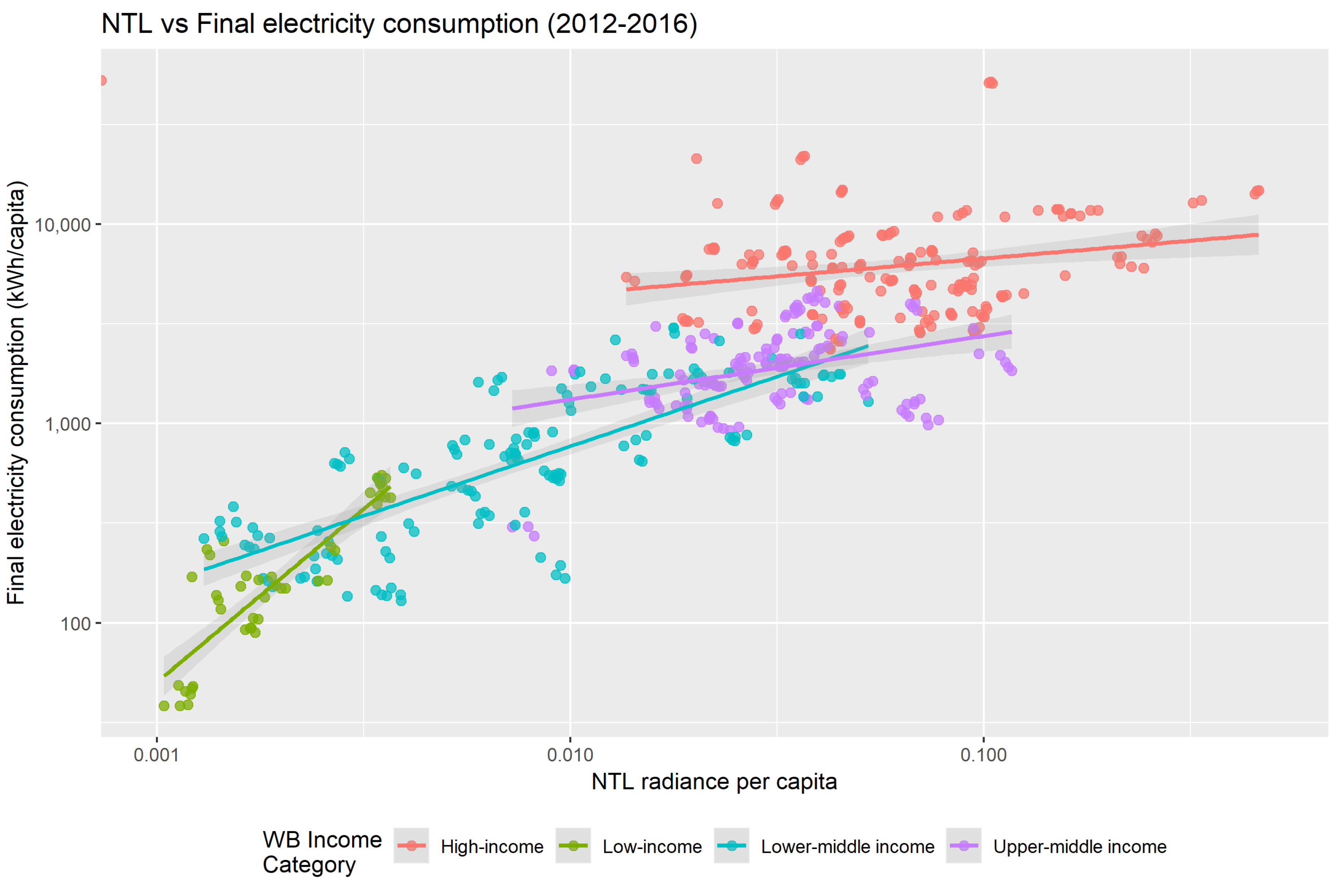
Here we report the result of log-log regressions (with heteroskedasticity-robust standard errors) run to assess the average explanatory power of NTL over the changes in the actual consumption levels within World Bank-defined income categories. The coefficients of the log-log specifications express the % change in the response variable as a result of a 1% change in the explanatory variable of interest, and thus the slope. Differentiating the specification with respect to the response variable results in , where the s measure the ceteris paribus % predicted change in the response variable (here, electricity consumption) for a 1% change in the explanatory variable of interest, i.e., sum of NTL radiance. This is what in economic terms is referred to as an elasticity. In both cases, reported regressions are those run with TFC as the response variable. The Appendix A reports results for the two other sub-categories of power consumption considered (commercial and public and residential). Figure 3 shows the scatterplot and linear fit for the log-log specification by income category, where each observation across the 2012–2016 period is reported for each country. Longitudinal regression results for TFC are reported in Table 3, Table 4, Table 5 and Table 6. Column 1 refers to a pooled OLS log-log specification, column 2 adds country-fixed-effects (which can be interpreted as a demeaning factor, i.e., a set of dummy variables controlling for the mean electricity consumption of each country), and column 3 also includes year-fixed-effects.
Regression results show that—when linking TFC and sum of NTL radiance in a pooled OLS regression—the relationship is positive and highly significant across income categories, with estimates in the 0.67–1.53 range. The highest coefficient is found for low-income countries (Table 3), and the lowest for high-income countries (Table 6), highlighting a general gradual decoupling of the total final electricity consumption from the lighting component across income categories. Nonetheless, when switching to fixed-effects specifications and therefore looking at the within-country interannual variations, the high statistical significance of the NTL coefficient persists only for lower-middle income countries (Table 3) and—limited to the country fixed-effects only specification—to upper-middle income countries (Table 5). While detailed discussion of this finding is offered in the Discussion section, we believe it likely reflects the fact that low-income countries might be affected by issues of data quality and low interannual heterogeneity in the five-year period for which the data is available, while in higher-middle and high income countries a decoupling in the relationship between light radiance and actual power consumption is expected (as partially confirmed from the pooled OLS results).
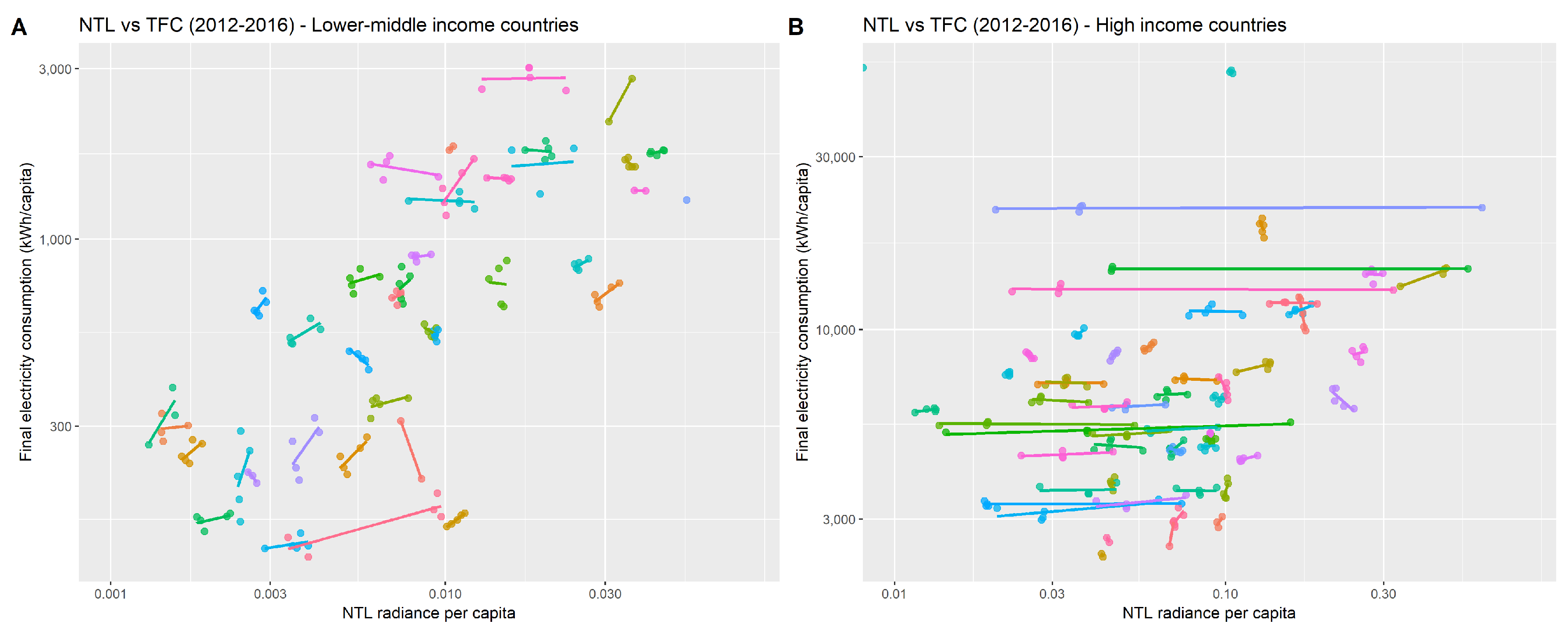
It is necessary to remark that in regression specifications (1) (log-log), the log of NTL coefficients show the ability to predict TFC from NTL, no matter the year or the country under analysis. Therefore, the estimators reflect the slopes of the lines of Figure 3. On the other hand, for specifications (2) (country fixed-effects, where the country-specific mean value across years is subtracted from each observation), the regression coefficients show the average ability to predict TFC from NTL within each country in that income category, i.e., they do not explain the overall heterogeneity in TFC, but only the changes from year to year within each country (the coefficient is thus a within-estimator). Since in the five-year period under examination we generally observe little variation within each country (at least in relative terms, i.e., compared to the large amount of variation between countries), adding country fixed-effects dramatically increases the fraction of total variance explained. Nonetheless, there still is some residual standard error to be explained, and we test the capacity of NTL to address precisely that residual (small relatively to the between county-heterogeneity, but here considered in absolute terms). The fact that variables are not dropped due to potential multicollinearity is reassuring in this sense. Figure 4 shows the analysis of specifications (2) with scatterplots and linear fits for (A) lower-middle income and (B) high-income countries. In particular, it shows how the within-country variation in TFC for a number of lower-middle income countries (but not all of them) is predicted effectively by NTL, while for the case of high-income countries, relationships appear flat, underpinning the (in)significance of regression coefficients of specifications (2). Finally, when considering specifications (3) (country and year fixed-effects), on the top of country fixed-effects we also add year dummies to control for those factors which are constant to all countries in each year but change from year to year, i.e., mostly data quality due to calibration of satellite.
Concerning regression diagnostics, it must be noted that the coefficient being close to 1 in the fixed-effect regression is caused by the limited amount of heterogeneity in the within-country data for the change in the TFC of electricity between 2012 and 2016. Adding fixed-effects to the specification makes the coefficient for the log of NTL fall substantially and the go close to 1. The residual standard error metric shows that there is indeed a fraction of unexplained heterogeneity (the should not be taken as a reference in this specific setting), the high statistical significance of the log(NTL) coefficient even under the fixed-effects specification in the context of lower-middle income countries is the most interesting result, because it shows that NTL are capable of capturing those small changes in the level of consumption within countries between one year and the other. The F Statistic—useful for comparing specifications as it sheds light on the significance of multiple coefficients at the same time—underpins our results. For instance, for low-income countries it shows that switching from the country-fixed-effects to the year and country-fixed-effects specification has a positive impact on the capacity of the model to explain the response variable, and thus that year fixed-effects contribute to explaining more variance than the country fixed-effects only.
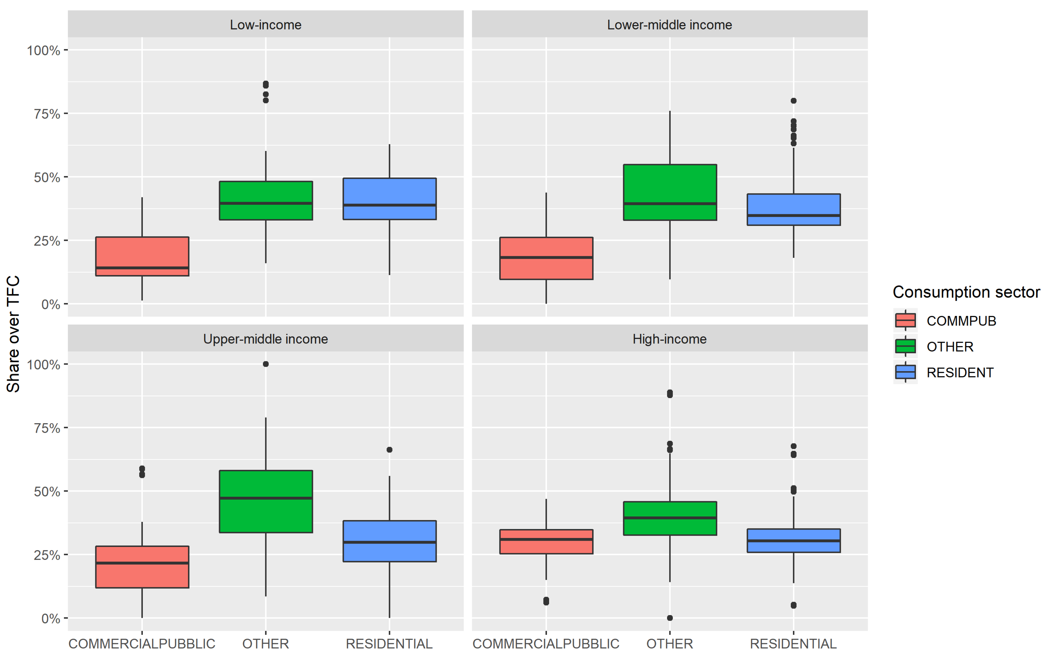
Figure 5 shows the distribution of the share of commercial and public electricity consumption (COMMPUB) and residential electricity consumption (RESIDENT) consumption over TFC by the four income categories considered. It shows how—as income increases—the spread between the two categories tends to close, with COMMPUB becoming dominant or comparable to RESIDENT in high-income countries.
The graph supports the understanding of our results, as it sheds some light on the varying significance of lighting across income categories. Detected NTL radiance stems from public street and road lighting, and from private buildings. Satellite data has been found to be suitable to detect both public [38,39] and indoor light [40], and therefore can potentially shed useful information on both components.
However, it has to be remembered that differences exist across countries in the procedures to collect and elaborate statistical data. For this reason, although the data are grouped in a common framework, some potential minor differences remain in the sector classifications of energy consumption. Thus, we believe that the use of total final consumption is a better indicator across multiple countries. For the same reason, to draw detailed conclusions on the type of lights that are actually captured would require a more detailed analysis at country or local scale.
4.2. Regional Clustering
To test if significant differences affect different regions of the world in the TFC-NTL relationship (e.g., due to cultural, infrastructure and development clustering), here (Table 7) we report the results of the regressions specifications implementing interaction terms between each macro-region and NTL intensity. Similarly to income-category clustering, Figure 6 shows the scatterplot and linear fit for the log-log specification by region, where values for each countries are averaged across the 2012–2016 period.
Results show that once fixed-effects are added, the main effect of the interaction term for log(NTL) becomes insignificant, but the interaction effects across log(NTL) and region remains positive and highly significant in Sub-Saharan Africa, Middle-East and North Africa, Latin America and the Caribbeans, and East Asia and the Pacific, with elasticities in the 0.34–0.75 range. In particular, the highest effect is found for East Asia and the Pacific and the lowest for Middle East and North Africa. Conversely, interaction coefficients for North America, South Asia and Europe are insignificant. Conversely, changes in Europe, North America and South Asia are not successfully predicted by NTL.
Comparing results with regressions for other consumption categories found in the Appendix A reveals substantially similar patterns in terms of significance. The key discrepancies is that while lower-middle income countries exhibit highly significant coefficients also for residential (0.21) and commercial and public (0.34) sectors, RESIDENT AND COMMPUB coefficients for upper-middle income countries are not significant even under the country-fixed-effects only specification. On the other hand, we observe a 10% significant coefficient for the country-fixed-effects specification for commercial and public consumption in high-income countries, although the observed coefficient (0.01) is particularly low and thus not deemed a robust result. Across regional-level outcomes, for the case of residential consumption, the same results that were found for TFC in terms of which interaction term coefficients are observed for the RESIDENT variable as statistically significant. However, in this case only two regions exhibit a very high significance, namely East Asia and the Pacific (0.59), and Sub-Saharan Africa (0.36). Conversely, with regards to commercial and public consumption, only NTL in East Asia and the Pacific are found to be highly significant predictors of interannual, within-country consumption level changes, with a 5% significant coefficient of 1.17.
5. Discussion and Conclusions
We have assessed the capacity of exploiting the interannual variation in VIIRS night-time light radiance to predict changes in the national electricity consumption change during the 2012–2016 period. Our results for TFC have highlighted that the approach is successful in lower-middle income countries, for which a coefficient is found in the country-year demeaning specification, and only partially in upper-middle income countries (country-fixed-effects coefficient of only significant at a 10% level), but not across other income categories. We believe that low-income countries might be affected by (i) issues of data quality (ii) little interannual heterogeneity in the five-year period for which the data is available, while in higher-middle and high income countries a decoupling in the relationship between light radiance and actual power consumption is the hypothesized reason for the insignificance of the regression coefficient. This result finds evidence in the pooled OLS specifications, which look into overall changes and not into the within-country variation. Here, the magnitude of the regression coefficient is declining as one moves up across income categories. This is in line with the initial hypothesis. In a similar fashion, we have found that macro-regions where the relation does not hold are those with the countries with the highest consumption and levels of per-capita incomes across the world, namely North America and Europe, but also the exception of South Asia (including India, Bangladesh, Pakistan, Sri Lanka, and Nepal). Conversely, the approach seems particularly suitable for East Asia and Latin America, for which the highest and most significant coefficients are found.
Research Prospects
One of the key objectives of this paper has been to carry out exploratory analysis for the capacity of NTL to predict the change in power consumption within a country. This is particularly interesting in the perspective of applying the methodology at finer spatio-temporal scales (e.g., in a number of developing countries at a monthly scale) and built an ad-hoc model which, once appropriately calibrated on historical data, can produce continuous estimates of energy consumption as new data is published. The upcoming release of a new generation of high-resolution, monthly NTL data product, the VIIRS-based VNP 46 Black Marble [4], could allow mitigating a substantial part of the issues in the raw data discussed in the Methods section of this paper. Furthermore, the validation with region or province level data on consumption in tight cooperation with local power supply utilities could render the model even more effective and insightful for the specific location under examination. At the same time, the national scale, yearly estimation approach could also be improved through the development of better algorithms to clean data and remove non-electric detected light, such as flaring, calibration noise, and albedo and land cover.
Author Contributions
Conceptualization, G.F. and M.N.; methodology, G.F. and M.N.; data extraction and statistic analysis, G.F.; visualization, M.N.; writing—original draft preparation, G.F.; writing—review and editing, G.F. and M.N.
Funding
This research received no external funding.
Acknowledgments
Support from the Fondazione Eni Enrico Mattei is gratefully acknowledged.
Conflicts of Interest
The authors declare no conflict of interest.
Source Code
The Javascript code written in Google Earth Engine to process the night-time light raster files in hosted at the following repository: https://github.com/giacfalk/VIIRS_electricity_assessment.
Abbreviations
The following abbreviations are used in this manuscript:
| COMMPUB | Commercial and public electricity consumption |
| DMSP-OLS | Defence Meteorological Satellite Program-Operational Linescan |
| DNB | Day-night band |
| GNI | Gross National Income |
| NPP | Suomi National Polar-orbiting Partnership |
| OECD | Organisation for Economic Co-operation and Development |
| OLS | Ordinary Least Squares regression |
| NASA | National Aeronautics and Space Administration |
| NOAA | National Oceanic and Atmospheric Administration |
| NTL | Night-time lights |
| RESIDENT | Residential electricity consumption |
| TFC | Total final electricity consumption |
| VIIRS | Visible Infrared Imager Radiometer Suite |
Appendix A
Appendix A.1. Regression Tables

Table A1.
Regression for COMMPUB—Low-income countries.
| Dependent Variable: | |||
|---|---|---|---|
| Log of Total Final Consumption of electricity | |||
| (1) | (2) | (3) | |
| (Log-log) | (Country fixed-effects) | (Country and year fixed-effects) | |
| Log of NTL | 1.104 *** | 0.363 | −0.021 |
| (0.178) | (0.611) | (0.678) | |
| Constant | −4.234 ** | ||
| (1.854) | |||
| Country fixed-effects? | No | Yes | Yes |
| Year fixed-effects? | No | No | Yes |
| Observations | 50 | 50 | 50 |
| R | 0.4433 | 0.9984 | 0.9986 |
| Adjusted R | 0.4317 | 0.9979 | 0.9978 |
| Residual Std. Error | 0.877 (df = 48) | 0.336 (df = 37) | 0.341 (df = 33) |
| F Statistic | 38.223 *** (df = 1; 48) | 1809.817 *** (df = 13; 37) | 1344.745 *** (df = 17; 33) |
Note: * ; ** ; *** .
Table A2.
Regression for COMMPUB—Lower-middle income countries.
| Dependent Variable: | |||
|---|---|---|---|
| Log of Total Final Consumption of electricity | |||
| (1) | (2) | (3) | |
| (Log-log) | (Country fixed-effects) | (Country and year fixed-effects) | |
| Log of NTL | 0.853 *** | 0.363 ** | 0.336 ** |
| (0.040) | (0.140) | (0.145) | |
| Constant | −1.122 ** | ||
| (0.495) | |||
| Country fixed-effects? | No | Yes | Yes |
| Year fixed-effects? | No | No | Yes |
| Observations | 142 | 142 | 142 |
| R | 0.7664 | 0.9997 | 0.9997 |
| Adjusted R | 0.7647 | 0.9996 | 0.9996 |
| Residual Std. Error | 0.659 (df = 140) | 0.192 (df = 109) | 0.193 (df = 105) |
| F Statistic | 459.267 *** (df = 1; 140) | 10,607.090 *** (df = 33; 109) | 9298.249 *** (df = 37; 105) |
Note: * ; ** ; *** .
Table A3.
Regression for COMMPUB—Higher-middle income countries.
| Dependent Variable: | |||
|---|---|---|---|
| Log of Total Final Consumption of electricity | |||
| (1) | (2) | (3) | |
| Log of NTL | 0.821 *** | 0.028 | 0.051 |
| (0.049) | (0.311) | (0.345) | |
| Constant | −0.685 | ||
| (0.626) | |||
| Country fixed-effects? | No | Yes | Yes |
| Year fixed-effects? | No | No | Yes |
| Observations | 128 | 128 | 128 |
| R | 0.6934 | 0.9994 | 0.9994 |
| Adjusted R | 0.691 | 0.9992 | 0.9992 |
| Residual Std. Error | 0.850 (df = 126) | 0.280 (df = 98) | 0.284 (df = 94) |
| F Statistic | 284.954 *** (df = 1; 126) | 5373.881 *** (df = 30; 98) | 4603.861 *** (df = 34; 94) |
Note: * ; ** ; *** .
Table A4.
Regression for COMMPUB—High-income countries.
| Dependent Variable: | |||
|---|---|---|---|
| Log of Total Final Consumption of electricity | |||
| (1) | (2) | (3) | |
| (Log-log) | (Country fixed-effects) | (Country and year fixed-effects) | |
| Log of NTL | 0.683 *** | 0.010 * | 0.006 |
| (0.035) | (0.005) | (0.005) | |
| Constant | 1.990 *** | ||
| (0.474) | |||
| Country fixed-effects? | No | Yes | Yes |
| Year fixed-effects? | No | No | Yes |
| Observations | 191 | 191 | 191 |
| R | 0.6683 | 1.000 | 1.000 |
| Adjusted R | 0.6666 | 1.000 | 1.000 |
| Residual Std. Error | 0.897 (df = 189) | 0.054 (df = 150) | 0.048 (df = 146) |
| F Statistic | 380.843 *** (df = 1; 189) | 206,386.200 *** (df = 41; 150) | 231,696.900 *** (df = 45; 146) |
Note: * ; ** ; *** .
Table A5.
Regression for COMMPUB—regional clustering.
| Dependent Variable: | |||
|---|---|---|---|
| Log of Total Final Consumption of electricity | |||
| (1) | (2) | (3) | |
| Log of NTL | 0.844 *** | 0.091 | 0.065 |
| (0.107) | (0.188) | (0.196) | |
| Central and Eastern Europ | −0.876 | 7.451 *** | 7.705 *** |
| (1.343) | (2.135) | (2.215) | |
| East Asia and the Pacific | −2.504 ** | −9.202 | −6.435 |
| (0.980) | (6.728) | (6.910) | |
| Europe | 3.349 *** | 11.354 *** | 11.370 *** |
| (0.500) | (0.271) | (0.277) | |
| Latin America and Caribbeans | −2.670 *** | 0.369 | 2.516 |
| (0.599) | (7.744) | (7.873) | |
| Middle East and North Africa | −0.755 | 1.914 | 2.000 |
| (0.782) | (2.236) | (2.237) | |
| North America | −11.767 * | 15.299 *** | 15.696 *** |
| (6.635) | (2.764) | (2.780) | |
| South Asia | −1.035 | 7.967 | 8.848 |
| (0.984) | (6.815) | (6.909) | |
| Sub-Saharan Africa | −1.237 ** | 9.765 *** | 10.987 *** |
| (0.611) | (3.210) | (3.281) | |
| Log of NTL × East Asia and the Pacific | 0.197 | 1.351 ** | 1.174 ** |
| (0.130) | (0.523) | (0.539) | |
| Log of NTL × Europe | −0.258 ** | −0.081 | −0.060 |
| (0.114) | (0.189) | (0.195) | |
| Log of NTL × Latin America and Caribbeans | 0.123 | 0.626 | 0.476 |
| (0.117) | (0.652) | (0.668) | |
| Log of NTL × Middle East and North Africa | −0.034 | 0.387 | 0.403 |
| (0.122) | (0.264) | (0.267) | |
| Log of NTL × North America | 0.659 * | −0.085 | −0.084 |
| (0.399) | (0.245) | (0.247) | |
| Log of NTL × South Asia | 0.007 | 0.103 | 0.062 |
| (0.131) | (0.527) | (0.543) | |
| Log of NTL × Sub-Saharan Africa | −0.005 | −0.210 | −0.300 |
| (0.121) | (0.350) | (0.360) | |
| Country fixed-effects? | No | Yes | Yes |
| Year fixed-effects? | No | No | Yes |
| Observations | 519 | 519 | 519 |
| R | 0.9947 | 0.9997 | 0.9997 |
| Adjusted R | 0.9946 | 0.9996 | 0.9996 |
| Residual Std. Error | 0.744 (df = 503) | 0.201 (df = 407) | 0.201 (df = 403) |
| F Statistic | 5926.033 *** (df = 16; 503) | 11,626.550 *** (df = 112; 407) | 11,260.480 *** (df = 116; 403) |
Note: * ; ** ; *** .
Table A6.
Regression for RESIDENT—Low-income countries.
| Dependent Variable: | |||
|---|---|---|---|
| Log of Total Final Consumption of electricity | |||
| (1) | (2) | (3) | |
| (Log-log) | (Country fixed-effects) | (Country and year fixed-effects) | |
| Log of NTL | 1.127 *** | 0.330 | 0.082 |
| (0.097) | (0.247) | (0.215) | |
| Constant | −3.526 *** | ||
| (1.008) | |||
| Country fixed-effects? | No | Yes | Yes |
| Year fixed-effects? | No | No | Yes |
| Observations | 50 | 50 | 50 |
| R | 0.7376 | 0.9998 | 0.9999 |
| Adjusted R | 0.7322 | 0.9998 | 0.9998 |
| Residual Std. Error | 0.477 (df = 48) | 0.136 (df = 37) | 0.108 (df = 33) |
| F Statistic | 134.948 *** (df = 1; 48) | 13,997.790 *** (df = 13; 37) | 16,915.650 *** (df = 17; 33) |
Note: * ; ** ; *** .
Table A7.
Regression for RESIDENT—Lower-middle income countries.
| Dependent Variable: | |||
|---|---|---|---|
| Log of Total Final Consumption of electricity | |||
| (1) | (2) | (3) | |
| Log of NTL | 0.915 *** | 0.304 *** | 0.205 *** |
| (0.033) | (0.086) | (0.073) | |
| Constant | −1.153 *** | ||
| (0.411) | |||
| Country fixed-effects? | No | Yes | Yes |
| Year fixed-effects? | No | No | Yes |
| Observations | 142 | 142 | 142 |
| R | 0.8468 | 0.9999 | 0.9999 |
| Adjusted R | 0.8457 | 0.9999 | 0.9999 |
| Residual Std. Error | 0.547 (df = 140) | 0.118 (df = 109) | 0.098 (df = 105) |
| F Statistic | 767.618 *** (df = 1; 140) | 32,611.740 *** (df = 33; 109) | 42,417.700 *** (df = 37; 105) |
Note: * ; ** ; *** .
Table A8.
Regression for RESIDENT—Higher-middle income countries.
| Dependent Variable: | |||
|---|---|---|---|
| Log of Total Final Consumption of electricity | |||
| (1) | (2) | (3) | |
| (Log-log) | (Country fixed-effects) | (Country and year fixed-effects) | |
| log(light_sum) | 0.779 *** | 0.164 ** | 0.054 |
| (0.028) | (0.078) | (0.061) | |
| Constant | 0.144 | ||
| (0.355) | |||
| Country fixed effects? | No | Yes | Yes |
| Year fixed effects? | No | No | Yes |
| Observations | 143 | 143 | 143 |
| R | 0.8506 | 1.000 | 1.000 |
| Adjusted R | 0.8495 | 1.000 | 1.000 |
| Residual Std. Error | 0.502 (df = 141) | 0.072 (df = 109) | 0.051 (df = 105) |
| F Statistic | 802.566 *** (df = 1; 141) | 85,751.280 *** (df = 34; 109) | 151,812.900 *** (df = 38; 105) |
Note: * ; ** ; *** .
Table A9.
Regression for RESIDENT—High-income countries.
| Dependent Variable: | |||
|---|---|---|---|
| Log of Total Final Consumption of electricity | |||
| (1) | (2) | (3) | |
| (Log-log) | (Country fixed-effects) | (Country and year fixed-effects) | |
| log(light_sum) | 0.713 *** | 0.007 | 0.003 |
| (0.037) | (0.005) | (0.005) | |
| Constant | 1.609 *** | ||
| (0.502) | |||
| Country fixed effects? | No | Yes | Yes |
| Year fixed effects? | No | No | Yes |
| Observations | 191 | 191 | 191 |
| R | 0.662 | 1.000 | 1.000 |
| Adjusted R | 0.6602 | 1.000 | 1.000 |
| Residual Std. Error | 0.949 (df = 189) | 0.048 (df = 150) | 0.046 (df = 146) |
| F Statistic | 370.164 *** (df = 1; 189) | 260,361.200 *** (df = 41; 150) | 251,062.300 *** (df = 45; 146) |
Note: * ; ** ; *** .
Table A10.
Regression for RESIDENT—regional clustering.
| Dependent Variable: | |||
|---|---|---|---|
| Log of Total Final Consumption of electricity | |||
| (1) | (2) | (3) | |
| (Log-log) | (Country fixed-effects) | (Country and year fixed-effects) | |
| Log of NTL | 0.631 *** | 0.089 | 0.036 |
| (0.088) | (0.079) | (0.074) | |
| Central and Eastern Europ | 2.358 ** | 8.378 *** | 8.924 *** |
| (1.101) | (0.898) | (0.835) | |
| East Asia and the Pacific | −0.643 | −1.494 | 3.405 |
| (0.803) | (2.830) | (2.604) | |
| Europe | 3.099 *** | 11.871 *** | 11.916 *** |
| (0.410) | (0.114) | (0.104) | |
| Latin America and Caribbeans | −1.435 *** | −0.607 | 3.136 |
| (0.491) | (3.258) | (2.967) | |
| Middle East and North Africa | 0.175 | 6.495 *** | 6.675 *** |
| (0.641) | (0.941) | (0.843) | |
| North America | −7.725 | 15.752 *** | 16.509 *** |
| (5.440) | (1.163) | (1.048) | |
| South Asia | 0.059 | 7.817 *** | 9.257 *** |
| (0.807) | (2.867) | (2.603) | |
| Sub-Saharan Africa | −0.865 * | 2.637 * | 4.812 *** |
| (0.501) | (1.350) | (1.236) | |
| Log of NTL × East Asia and the Pacific | 0.287 *** | 0.891 *** | 0.585 *** |
| (0.107) | (0.220) | (0.203) | |
| Log of NTL × Europe | −0.032 | −0.082 | −0.037 |
| (0.093) | (0.080) | (0.074) | |
| Log of NTL × Latin America and Caribbeans | 0.267*** | 0.734 *** | 0.481 * |
| (0.096) | (0.274) | (0.252) | |
| Log of NTL × Middle East and North Africa | 0.152 | 0.140 | 0.173 * |
| (0.100) | (0.111) | (0.101) | |
| Log of NTL × North America | 0.649 ** | −0.107 | −0.100 |
| (0.327) | (0.103) | (0.093) | |
| Log of NTL × South Asia | 0.220 ** | 0.207 | 0.152 |
| (0.108) | (0.222) | (0.204) | |
| Log of NTL × Sub-Saharan Africa | 0.237 ** | 0.511 *** | 0.359 *** |
| (0.099) | (0.147) | (0.136) | |
| Country fixed-effects? | No | Yes | Yes |
| Year fixed-effects? | No | No | Yes |
| Observations | 519 | 519 | 519 |
| R | 0.9965 | 0.9999 | 1.000 |
| Adjusted R | 0.9964 | 0.9999 | 0.9999 |
| Residual Std. Error | 0.610 (df = 503) | 0.085 (df = 407) | 0.076 (df = 403) |
| F Statistic | 9478.520 *** (df = 16; 503) | 70,516.450 *** (df = 112; 407) | 85,118.370 *** (df = 116; 403) |
Note: * ; ** ; *** .
Appendix A.2. Additional Figures
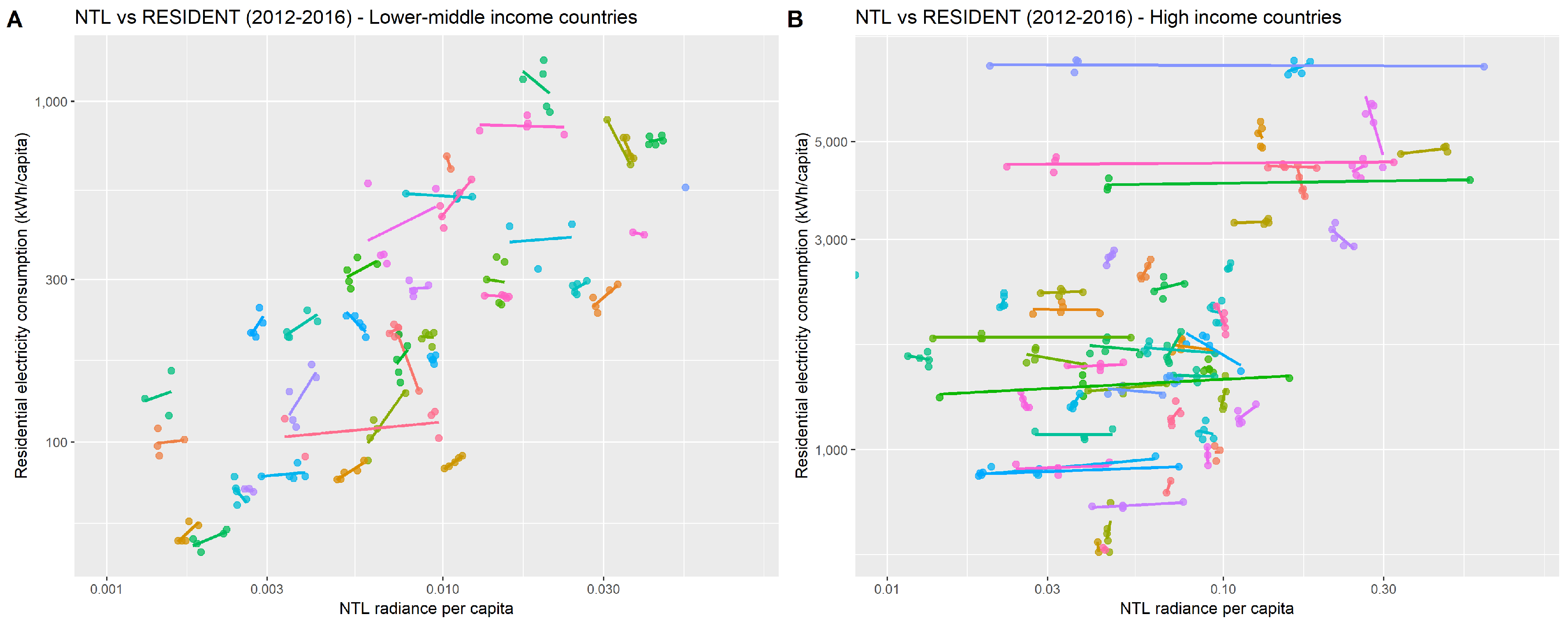
Figure A1.
NTL vs. RESIDENT for (A) lower-middle income and (B) high-income countries (annual values between 2012–2016).
Figure A1.
NTL vs. RESIDENT for (A) lower-middle income and (B) high-income countries (annual values between 2012–2016).

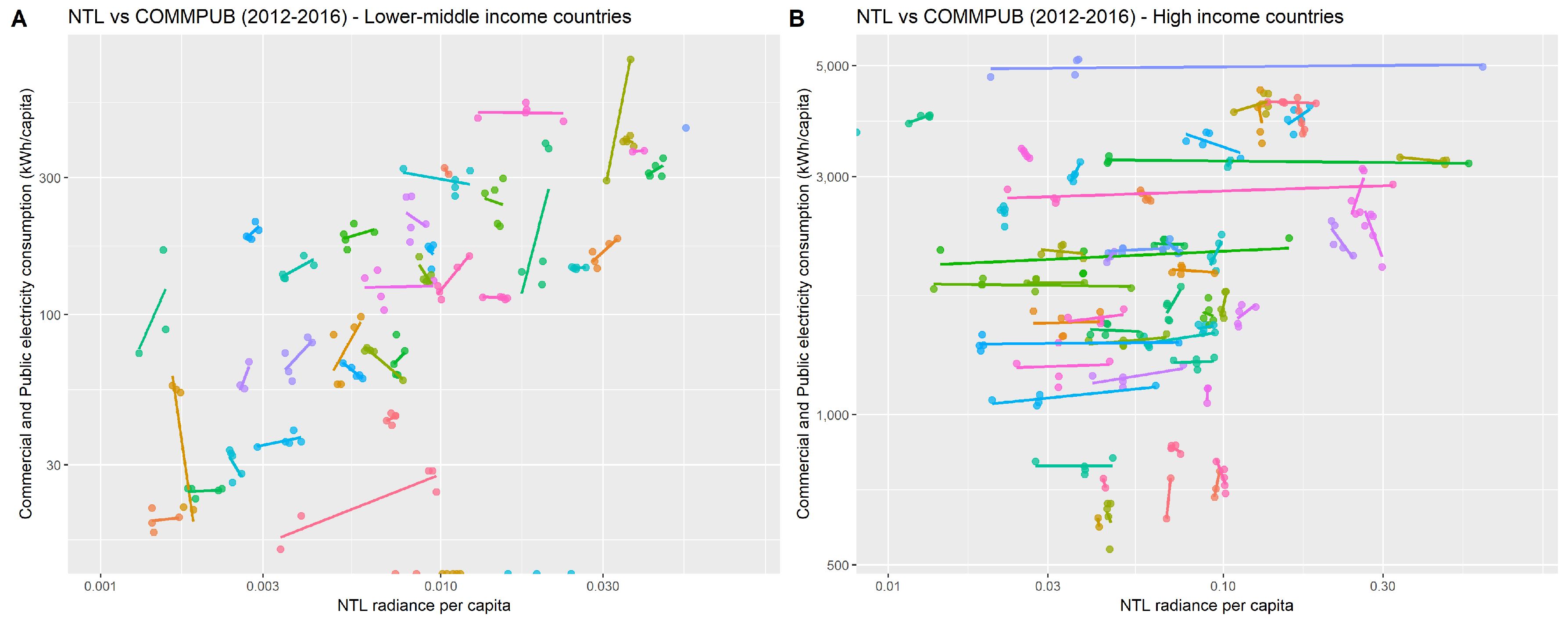
Figure A2.
NTL vs. COMMPUB for (A) lower-middle income and (B) high-income countries (annual values between 2012–2016).
Figure A2.
NTL vs. COMMPUB for (A) lower-middle income and (B) high-income countries (annual values between 2012–2016).

References
- Bennett, M.M.; Smith, L.C. Advances in using multitemporal night-time lights satellite imagery to detect, estimate, and monitor socioeconomic dynamics. Remote Sens. Environ. 2017, 192, 176–197. [Google Scholar] [CrossRef]
- Bruederle, A.; Hodler, R. Nighttime lights as a proxy for human development at the local level. PLoS ONE 2018, 13, e0202231. [Google Scholar] [CrossRef] [PubMed]
- Baugh, K.; Hsu, F.C.; Elvidge, C.D.; Zhizhin, M. Nighttime lights compositing using the VIIRS day-night band: Preliminary results. Proc. Asia-Pac. Adv. Netw. 2013, 35, 70–86. [Google Scholar] [CrossRef]
- Román, M.O.; Wang, Z.; Sun, Q.; Kalb, V.; Miller, S.D.; Molthan, A.; Schultz, L.; Bell, J.; Stokes, E.C.; Pandey, B.; et al. NASA’s Black Marble nighttime lights product suite. Remote Sens. Environ. 2018, 210, 113–143. [Google Scholar] [CrossRef]
- Townsend, A.C.; Bruce, D.A. The use of night-time lights satellite imagery as a measure of Australia’s regional electricity consumption and population distribution. Int. J. Remote Sens. 2010, 31, 4459–4480. [Google Scholar] [CrossRef]
- Coscieme, L.; Pulselli, F.M.; Bastianoni, S.; Elvidge, C.D.; Anderson, S.; Sutton, P.C. A Thermodynamic Geography: Night-Time Satellite Imagery as a Proxy Measure of Emergy. Ambio 2014, 43, 969–979. [Google Scholar] [CrossRef]
- He, C.; Ma, Q.; Li, T.; Yang, Y.; Liu, Z. Spatiotemporal dynamics of electric power consumption in Chinese Mainland from 1995 to 2008 modeled using DMSP/OLS stable nighttime lights data. J. Geogr. Sci. 2012, 22, 125–136. [Google Scholar] [CrossRef]
- Fehrer, D.; Krarti, M. Spatial distribution of building energy use in the United States through satellite imagery of the earth at night. Build. Environ. 2018. [Google Scholar] [CrossRef]
- Shi, K.; Yu, B.; Huang, C.; Wu, J.; Sun, X. Exploring spatiotemporal patterns of electric power consumption in countries along the Belt and Road. Energy 2018, 150, 847–859. [Google Scholar] [CrossRef]
- Baldwin, H.B.; Klug, M.; Tapracharoen, K.; Visudchindaporn, C. Utilizing Suomi NPP’s Day-Night Band to Assess Energy Consumption in Rural and Urban Areas as an Input for Poverty Analysis. In Proceedings of the AGU Fall Meeting, New Orleans, LA, USA, 11–15 December 2017. AGU Fall Meeting Abstracts. [Google Scholar]
- Wang, Z.; Román, M.O.; Sun, Q.; Molthan, A.L.; Schultz, L.A.; Kalb, V.L. Monitoring Disaster-Related Power Outages Using Nasa Black Marble Nighttime Light Product. ISPRS Int. Arch. Photogramm. Remote Sens. Spat. Inf. Sci. 2018, XLII-3, 1853–1856. [Google Scholar] [CrossRef]
- Mann, M.L.; Melaas, E.K.; Malik, A. Using VIIRS day/night band to measure electricity supply reliability: Preliminary results from Maharashtra, India. Remote Sens. 2016, 8, 711. [Google Scholar] [CrossRef]
- Min, B.; Gaba, K.M. Tracking electrification in Vietnam using nighttime lights. Remote Sens. 2014, 6, 9511–9529. [Google Scholar] [CrossRef]
- Min, B.; Gaba, K.M.; Sarr, O.F.; Agalassou, A. Detection of rural electrification in africa using DMSP-OLS night lights imagery. Int. J. Remote Sens. 2013, 34, 8118–8141. [Google Scholar] [CrossRef]
- Burlig, F.; Preonas, L. Out of the Darkness and Into the Light? Development Effects of Rural Electrification; Revised October 2016; Energy Institute: Haas, Syria, 2016; pp. 1–66. [Google Scholar]
- Doll, C.N.; Pachauri, S. Estimating rural populations without access to electricity in developing countries through night-time light satellite imagery. Energy Policy 2010, 38, 5661–5670. [Google Scholar] [CrossRef]
- Elvidge, C.D.; Baugh, K.E.; Sutton, P.C.; Bhaduri, B.; Tuttle, B.T.; Ghosh, T.; Ziskin, D.; Erwin, E.H. Who’s in the Dark—Satellite Based Estimates of Electrification Rates. In Urban Remote Sensing; Yang, X., Ed.; John Wiley & Sons, Ltd.: Hoboken, NJ, USA, 2011; pp. 211–224. [Google Scholar] [CrossRef]
- Román, M.O.; Stokes, E.C. Holidays in lights: Tracking cultural patterns in demand for energy services. Earth’s Future 2015, 3, 182–205. [Google Scholar] [CrossRef] [PubMed] [Green Version]
- Henderson, J.V.; Storeygard, A.; Weil, D.N. Measuring economic growth from outer space. Am. Econ. Rev. 2012, 102, 994–1028. [Google Scholar] [CrossRef]
- Jean, N.; Burke, M.; Xie, M.; Davis, W.M.; Lobell, D.B.; Ermon, S. Machine Learning To Predict Poverty. Science 2016, 353, 790–794. [Google Scholar] [CrossRef]
- Wu, R.; Yang, D.; Dong, J.; Zhang, L.; Xia, F. Regional Inequality in China Based on NPP-VIIRS Night-Time Light Imagery. Remote Sens. 2018, 10, 240. [Google Scholar] [CrossRef]
- Doll, C.H.; Muller, J.P.; Elvidge, C.D. Night-time Imagery as a Tool for Global Mapping of Socioeconomic Parameters and Greenhouse Gas Emissions. AMBIO J. Hum. Environ. 2000, 29, 157–162. [Google Scholar] [CrossRef]
- Campos, I.; González-Gómez, L.; Villodre, J.; Calera, M.; Campoy, J.; Jiménez, N.; Plaza, C.; Sánchez-Prieto, S.; Calera, A. Mapping within-field variability in wheat yield and biomass using remote sensing vegetation indices. Precis. Agric. 2018, 1–23. [Google Scholar] [CrossRef]
- Fawzi, N.; Husna, V.; Helms, J. Measuring deforestation using remote sensing and its implication for conservation in Gunung Palung National Park, West Kalimantan, Indonesia. In IOP Conference Series: Earth and Environmental Science; IOP Publishing: Bristol, UK, 2018; Volume 149, p. 012038. [Google Scholar]
- Fragkias, M.; Lobo, J.; Seto, K.C. A comparison of nighttime lights data for urban energy research: Insights from scaling analysis in the US system of cities. Environ. Plan. B Urban Anal. City Sci. 2017, 44, 1077–1096. [Google Scholar] [CrossRef]
- Shi, K.; Yang, Q.; Fang, G.; Yu, B.; Chen, Z.; Yang, C.; Wu, J. Evaluating spatiotemporal patterns of urban electricity consumption within different spatial boundaries: A case study of Chongqing, China. Energy 2018, 167, 641–653. [Google Scholar] [CrossRef]
- Xiao, H.; Ma, Z.; Mi, Z.; Kelsey, J.; Zheng, J.; Yin, W.; Yan, M. Spatio-temporal simulation of energy consumption in China’s provinces based on satellite night-time light data. Applied Energy 2018, 231, 1070–1078. [Google Scholar] [CrossRef]
- IEA. World Energy Outlook 2018; Technical Report; IEA: Paris, France, 2018. [Google Scholar]
- Chen, X.; Nordhaus, W. A Test of the New VIIRS Lights Data Set: Population and Economic Output in Africa. Remote Sens. 2015, 7, 4937–4947. [Google Scholar] [CrossRef] [Green Version]
- Zhao, N. Seasonality and Decomposition of Monthly VIIRS-DNB Image Composites. 2018. Available online: https://aag.secure-abstracts.com/AAG%20Annual%20Meeting%202018/abstracts-gallery/11752 (accessed on 1 December 2018).
- Zhao, N.; Hsu, F.C.; Cao, G.; Samson, E.L. Improving accuracy of economic estimations with VIIRS DNB image products. Int. J. Remote Sens. 2017, 38, 5899–5918. [Google Scholar] [CrossRef]
- International Energy Agency. World Energy Balances; IEA: Paris, France, 2016. [Google Scholar] [CrossRef]
- Bank, W. World Bank Country and Lending Groups–World Bank Data Help Desk. 2018. Available online: https://datahelpdesk.worldbank.org/knowledgebase/articles/906519-world-bank-country-and-lending-groups (accessed on 15 November 2018).
- Gorelick, N.; Hancher, M.; Dixon, M.; Ilyushchenko, S.; Thau, D.; Moore, R. Google Earth Engine: Planetary-scale geospatial analysis for everyone. Remote Sens. Environ. 2017, 202, 18–27. [Google Scholar] [CrossRef]
- Levin, N.; Zhang, Q. A global analysis of factors controlling VIIRS nighttime light levels from densely populated areas. Remote Sens. Environ. 2017, 190, 366–382. [Google Scholar] [CrossRef]
- Elvidge, C.D.; Zhizhin, M.; Baugh, K.; Hsu, F.C.; Ghosh, T. Methods for global survey of natural gas flaring from visible infrared imaging radiometer suite data. Energies 2016, 9, 14. [Google Scholar] [CrossRef]
- The World Bank. Global Gas Flaring Reduction Partnership (GGFR); World Bank Group: Washington, DC, USA, 2018. [Google Scholar]
- De Miguel, A.S.; Zamorano, J.; Castaño, J.G.; Pascual, S. Evolution of the energy consumed by street lighting in Spain estimated with DMSP-OLS data. J. Quant. Spectrosc. Radiat. Transf. 2014, 139, 109–117. [Google Scholar] [CrossRef] [Green Version]
- Estrada-García, R.; García-Gil, M.; Acosta, L.; Bará, S.; Sanchez-de Miguel, A.; Zamorano, J. Statistical modelling and satellite monitoring of upward light from public lighting. Light. Res. Technol. 2016, 48, 810–822. [Google Scholar] [CrossRef] [Green Version]
- Hänel, A.; Doulos, L.; Schroer, S.; Gălăţanu, C.D.; Topalis, F. Sustainable outdoor lighting for reducing energy and light waste. In Proceedings of the 9th International Conference Improving Energy Efficiency in Commercial Buildings and Smart Communities, IEECB & SC, Frankfurt, Germany, 16–18 March 2016; Volume 16. [Google Scholar]
Figure 1.
Average annual per-capita total final consumption of electricity (TFC), worldwide.

Figure 2.
Average annual sum of light per capita, worldwide.

Figure 3.
Night-time light (NTL) vs. TFC by World Bank (WB) Income Category (annual values between 2012–2016).
Figure 3.
Night-time light (NTL) vs. TFC by World Bank (WB) Income Category (annual values between 2012–2016).

Figure 4.
NTL vs. TFC for (A) lower-middle income and (B) high-income countries (annual values between 2012–2016). Each color represents a separate country.
Figure 4.
NTL vs. TFC for (A) lower-middle income and (B) high-income countries (annual values between 2012–2016). Each color represents a separate country.

Figure 5.
Share of electricity consumption sectors over TFC, by income category. Commercial and public electricity consumption (COMMPUB), residential electricity consumption (RESIDENT).
Figure 5.
Share of electricity consumption sectors over TFC, by income category. Commercial and public electricity consumption (COMMPUB), residential electricity consumption (RESIDENT).

Figure 6.
NTL vs. TFC by region (average values 2012–2016).

Table 1.
Median sum of light in selected countries countries with and without floor correction.
| Country | Corrected | Non-Corrected | Percentage Change |
|---|---|---|---|
| Russia | 0.229 | 0.694 | −67.0% |
| Finland | 0.322 | 0.651 | −50.5% |
| Norway | 0.258 | 0.609 | −57.7% |
| Sweden | 0.165 | 0.365 | −54.8% |
| Iceland | 1.855 | 4.641 | −60.0% |
| Canada | 0.413 | 1.758 | −76.5% |
Table 2.
Mean sum of light with and without correction in top flaring countries and in control countries.
Table 2.
Mean sum of light with and without correction in top flaring countries and in control countries.
| Country | Corrected | Non-Corrected | Percentage Change |
|---|---|---|---|
| Algeria | 0.068 | 0.110 | −38.2% |
| Nigeria | 0.004 | 0.005 | −31.1% |
| Saudi Arabia | 3.149 | 3.335 | −5.6% |
| Iraq | 0.088 | 0.224 | −60.8% |
| Iran | 0.062 | 0.097 | −35.9% |
| Russia | 0.219 | 0.254 | −13.9% |
| United Kingdom | 0.050 | 0.051 | −0.7% |
| France | 0.066 | 0.067 | −1.7% |
| India | 0.005 | 0.005 | −1.5% |
| United States | 0.140 | 0.142 | −1.5% |
Table 3.
Low-income countries regression for TFC.
| Dependent Variable: | |||
|---|---|---|---|
| Log of total final consumption of electricity | |||
| (1) | (2) | (3) | |
| (Log-log) | (Country fixed-effects) | (Country and year fixed-effects) | |
| Log of NTL () | 1.526 *** | 0.398 | 0.177 |
| (0.067) | (0.263) | (0.251) | |
| Constant | −6.662 *** | ||
| (0.696) | |||
| Country fixed-effects? | No | Yes | Yes |
| Year fixed-effects? | No | No | Yes |
| Observations | 50 | 50 | 50 |
| R | 0.9153 | 0.9998 | 0.9999 |
| Adjusted R | 0.9136 | 0.9998 | 0.9998 |
| Residual Std. Error | 0.329 (df = 48) | 0.145 (df = 37) | 0.126 (df = 33) |
| F Statistic | 518.954 *** (df = 1; 48) | 15,625.980 *** (df = 13; 37) | 15,645.830 *** (df = 17; 33) |
Note: * ; ** ; *** .
Table 4.
Lower-middle income countries regression for TFC.
| Dependent Variable: | |||
|---|---|---|---|
| Log of total final consumption of electricity | |||
| (1) | (2) | (3) | |
| (Log-log) | (Country fixed-effects) | (Country and year fixed-effects) | |
| Log of NTL () | 0.912 *** | 0.336 *** | 0.233 *** |
| (0.036) | (0.074) | (0.059) | |
| Constant | −0.111 | ||
| (0.445) | |||
| Country fixed-effects? | No | Yes | Yes |
| Year fixed-effects? | No | No | Yes |
| Observations | 147 | 147 | 147 |
| R | 0.8174 | 0.9999 | 0.9999 |
| Adjusted R | 0.8161 | 0.9999 | 0.9999 |
| Residual Std. Error | 0.599 (df = 145) | 0.104 (df = 112) | 0.080 (df = 108) |
| F Statistic | 648.889 *** (df = 1; 145) | 48,912.520 *** (df = 35; 112) | 74,798.650 *** (df = 39; 108) |
Note: * ; ** ; *** .
Table 5.
Upper-middle income countries regression for TFC.
| Dependent Variable: | |||
|---|---|---|---|
| Log of Total Final Consumption of electricity | |||
| (1) | (2) | (3) | |
| (Log-log) | (Country fixed-effects) | (Country and year fixed-effects) | |
| Log of NTL () | 0.862 *** | 0.129 * | 0.039 |
| (0.029) | (0.071) | (0.061) | |
| Constant | 0.255 | ||
| (0.379) | |||
| Country fixed-effects? | No | Yes | Yes |
| Year fixed-effects? | No | No | Yes |
| Observations | 148 | 148 | 148 |
| R | 0.8542 | 1.000 | 1.000 |
| Adjusted R | 0.8532 | 1.000 | 1.000 |
| Residual Std. Error | 0.554 (df = 146) | 0.065 (df = 113) | 0.051 (df = 109) |
| F Statistic | 855.698 *** (df = 1; 146) | 127,312.800 *** (df = 35; 113) | 186,778.500 *** (df = 39; 109) |
Note: * ; ** ; *** .
Table 6.
High-income countries regression for TFC.
| Dependent Variable: | |||
|---|---|---|---|
| Log of total final consumption of electricity | |||
| (1) | (2) | (3) | |
| (Log-log) | (Country fixed-effects) | (Country and year fixed-effects) | |
| Log of NTL () | 0.665 *** | 0.005 | 0.001 |
| (0.036) | (0.004) | (0.004) | |
| Constant | 3.482 *** | ||
| (0.483) | |||
| Country fixed-effects? | No | Yes | Yes |
| Year fixed-effects? | No | No | Yes |
| Observations | 191 | 191 | 191 |
| R | 0.6479 | 1.000 | 1.000 |
| Adjusted R | 0.6461 | 1.000 | 1.000 |
| Residual Std. Error | 0.913 (df = 189) | 0.039 (df = 150) | 0.036 (df = 146) |
| F Statistic | 347.828 *** (df = 1; 189) | 471,777.300 *** (df = 41; 150) | 502,138.200 *** (df = 45; 146) |
Note: * ; ** ; *** .
Table 7.
Region clustering regression for TFC.
| Dependent Variable: | |||
|---|---|---|---|
| Log of total final consumption of electricity | |||
| (1) | (2) | (3) | |
| (Log-log) | (Country fixed-effects) | (Country and year fixed-effects) | |
| Log of NTL () | 0.741 *** | 0.008 | −0.034 |
| (0.082) | (0.074) | (0.066) | |
| Central and Eastern Europ | 2.061 ** | 11.906 *** | 12.394 *** |
| (1.033) | (0.962) | (0.864) | |
| East Asia and the Pacific | −1.373 ** | −0.378 | 3.179* |
| (0.690) | (2.074) | (1.828) | |
| Europe | 5.029 *** | 12.952 *** | 12.980 *** |
| (0.395) | (0.107) | (0.094) | |
| Latin America and Caribbeans | −1.329 *** | −1.359 | 2.385 |
| (0.474) | (3.049) | (2.677) | |
| Middle East and North Africa | 1.057 * | 5.675 *** | 5.888 *** |
| (0.603) | (0.877) | (0.759) | |
| North America | −5.697 | 16.870 *** | 17.563 *** |
| (5.245) | (1.088) | (0.946) | |
| South Asia | −0.165 | 10.763 *** | 12.294 *** |
| (0.778) | (2.684) | (2.350) | |
| Sub-Saharan Africa | −0.424 | 3.803 *** | 6.296 *** |
| (0.474) | (1.401) | (1.238) | |
| Log of NTL × East Asia and the Pacific | 0.317 *** | 0.966 *** | 0.746 *** |
| (0.098) | (0.167) | (0.148) | |
| Log of NTL × Europe | −0.189 ** | −0.003 | 0.033 |
| (0.088) | (0.074) | (0.066) | |
| Log of NTL × Latin America and Caribbeans | 0.237 *** | 0.950 *** | 0.685 *** |
| (0.090) | (0.257) | (0.227) | |
| Log of NTL × Middle East and North Africa | 0.040 | 0.321 *** | 0.340 *** |
| (0.094) | (0.104) | (0.091) | |
| Log of NTL × North America | 0.482 | −0.033 | −0.033 |
| (0.315) | (0.096) | (0.084) | |
| Log of NTL × South Asia | 0.205 ** | 0.128 | 0.055 |
| (0.102) | (0.207) | (0.184) | |
| Log of NTL × Sub-Saharan Africa | 0.183 ** | 0.514 *** | 0.348 *** |
| (0.093) | (0.136) | (0.121) | |
| Country fixed-effects? | No | Yes | Yes |
| Year fixed-effects? | No | No | Yes |
| Observations | 544 | 544 | 544 |
| R | 0.0.9975 | 1.000 | 1.000 |
| Adjusted R | 0.0.9974 | 1.000 | 1.000 |
| Residual Std. Error | 0.588 (df = 528) | 0.079 (df = 427) | 0.068 (df = 423) |
| F Statistic | 13,010.400 *** (df = 16; 528) | 98,231.090 *** (df = 117; 427) | 127,478.000 *** (df = 121; 423) |
Note: * ; ** ; *** .
© 2019 by the authors. Licensee MDPI, Basel, Switzerland. This article is an open access article distributed under the terms and conditions of the Creative Commons Attribution (CC BY) license (http://creativecommons.org/licenses/by/4.0/).
Share and Cite
MDPI and ACS Style
Falchetta, G.; Noussan, M. Interannual Variation in Night-Time Light Radiance Predicts Changes in National Electricity Consumption Conditional on Income-Level and Region. Energies 2019, 12, 456. https://doi.org/10.3390/en12030456
AMA Style
Falchetta G, Noussan M. Interannual Variation in Night-Time Light Radiance Predicts Changes in National Electricity Consumption Conditional on Income-Level and Region. Energies. 2019; 12(3):456. https://doi.org/10.3390/en12030456
Chicago/Turabian StyleFalchetta, Giacomo, and Michel Noussan. 2019. "Interannual Variation in Night-Time Light Radiance Predicts Changes in National Electricity Consumption Conditional on Income-Level and Region" Energies 12, no. 3: 456. https://doi.org/10.3390/en12030456
Note that from the first issue of 2016, this journal uses article numbers instead of page numbers. See further details here.