
Mapping Impacts of Human Activities from Nighttime Light on Vegetation Cover Changes in Southeast Asia

1
Jiangsu Provincial Key Laboratory of Geographic Information Technology, School of Geography and Ocean Science, Nanjing University, Nanjing 210093, China
2
Department of Geographic Information Science, Nanjing University, Nanjing 210093, China
3
Fenner School of Environment and Society, Australian National University, Canberra, ACT 2601, Australia
4
Collaborative Innovation Center for the South Sea Studies, Nanjing University, Nanjing 210093, China
*
Author to whom correspondence should be addressed.
Land 2021, 10(2), 185; https://doi.org/10.3390/land10020185
Submission received: 5 January 2021
/
Revised: 30 January 2021
/
Accepted: 3 February 2021
/
Published: 11 February 2021
(This article belongs to the Special Issue Remote Sensing Analysis of Agricultural Landscapes)
Abstract
:It is commonly believed that the impacts of human activities have decreased the natural vegetation cover, while some promotion of the vegetation growth has also been found. In this study, negative or positive correlations between human impacts and vegetation cover were tested in the Southeast Asia (SEA) region during 2012–2018. The Visible Infrared Imaging Radiometer Suite—Day/Night Band (VIIRS/DNB) nocturnal data were used as a measure of human activities and the moderate resolution imaging spectroradiometer (MODIS)/normalized difference vegetation index (NDVI) diurnal data were used as a measure of vegetation cover. The temporal segmentation method was introduced to calculate features of two sets of time series with spatial resolution of about 500 m, including the overall trend, maximum trend, start date, and change duration. The regions with large variation in human activities (V-change region) were first extracted by the Gaussian fitted method, and 8.64% of the entire SEA (VIIRS overall trend <−0.2 or >0.4) was set as the target analysis area. According to statistics, the average overall VIIRS trend for the V-change region in SEA was about 2.12, with a slight NDVI increment. The time lag effect was also found between vegetation cover and human impacts change, with an average of 10.26 months. Our results indicated a slight green overall trend in the SEA region over the most recent 7 years. The spatial pattern of our trend analysis results can be useful for vegetation management and regional planning.
1. Introduction
During the last decades of modern industrial societies, the world population has grown rapidly by 1.24% per year, and the rate dropped to 1.10% per year nowadays, still yielding an additional 83 million people annually [1,2]. The increasing population will require more urban or built-up areas for human development, and the global land and environment has been suffering measurable human pressures [3,4,5]. Especially for developing countries, the urbanization becomes the irreversible process during the last decades, and it will occupy a certain amount of vegetation cover, such as croplands, forest, and grassland [3,6,7]. This kind of land-use conversion has resulted in serious ecological problems, such as loss of the ecosystem services [8] and biodiversity reduction [9]. However, some researchers have also found a remarkable growing trend of vegetation cover [10], even in some urban areas [5,11]. This is mainly due to more attention to the environmental and ecological protection and scientific protection schemes, resulting in the vegetation cover increment [11,12,13]. Therefore, the positive or negative correlation between vegetation cover and human impacts is still under debate, and the magnitude of these correlations is ambiguous.
Vegetation dynamics and the influence of human impacts are both long-term and dynamic processes, and satellite-based datasets have provided opportunities for holistic monitoring at a larger spatial and temporal range [5,6,14,15]. Simply, the magnitude of human impacts can be approximately quantified as different land cover/use types from single or integrated diurnal remote sensing data [3,16]. Moreover, the satellite-derived nighttime light (NTL) can provide a uniform and convenient indicator to monitor and analyze the magnitude of human activities [17,18,19,20,21]. The intensity of NTL has proven strong correlations with human activities and socioeconomic parameters at multiple scales [22,23], such as urbanization [18,24], energy consumption [25], regional disparity [26], and declines in nocturnal activities by COVID-19 [19]. The Visible Infrared Imaging Radiometer Suite—Day/Night Band (VIIRS/DNB) nighttime lights data, launched in 2012, can detect nighttime lights with higher spatial and radiometric resolutions, with lighter problems of saturation, blooming, and on-board calibration [22,27]. Similarly, the remote sensing techniques can also be applied to map the large-scale vegetation cover dynamics [28,29]. The vegetation index (VI) from the remote sensing data products can measure the vegetation cover directly, such as Normalized Difference Vegetation Index (NDVI). Among all, Moderate Resolution Imaging Spectroradiometer (MODIS) data have the superior advantages in long-term analysis for temporal consistency and the uniform sensors [30].
According to the existing research, vegetation cover can be influenced by human factors and non-human factors, such as climate and the environment [11,31,32]. In this study, we only focus on the human impacts change that could be detected from NTL data, and areas with little human activity changes are excluded to minimize other influences. To evaluate the correlations of vegetation dynamics and human impact, the core problem is to find out the difference from spatial comparison [9]. However, few researchers have focused on the quantitative assessment of this correlation [16], and most of the existing research studies just directly combine NTL and NDVI datasets, based on negative correlations, for human footprint mapping and related information extraction [33,34,35]. Although some researchers have systematically studied the correlation between NTL changes and NDVI changes, these different analyses are mostly based on short time series or static imageries [11,27]. For these kinds of difference analysis, the derived features or differences are sometimes inaccurate mainly due to the natural vegetation phenology of NDVI data [36] and cloud cover of NTL data [37], along with other atmospheric scattering, geometric errors, and stray light problems. These data problems may result in large interannual variability of change detection when choosing different time nodes, and the time-series analysis can alleviate these problems [38]. Thus, the time series analysis between NTL data and NDVI data is necessary to reveal the vegetation response to human impacts quantitatively.
The time series analysis has proven successful in vegetation change detection, such as agricultural abandonment [39] and forest disturbance [40]. For NTL data, time series analysis is especially valuable for detecting, monitoring, and estimating the socioeconomic dynamics at various temporal and spatial scales [22,23,41]. For the annual seasonality influence of NDVI and NTL data, there are many existing mature methods or models to acquire the real overall trends, such as the Ordinary Least-Squares model [42], STMAP (Sorted Temporal Mixture Analysis with Post-classification) model [16], and the Theil–Sen median slope method [32,38]. However, for both human impacts and vegetation cover changes, the occurrence date of change may vary greatly in a certain studied time range, and there are sometimes multiple obvious changes with different change directions [40]. Meanwhile, changes of time series are not always gradual and constant, and there are some abrupt changes [43]. Thus, the segmentation of the time series is necessary to identify the temporal pattern [44]. Secondly, time lag effects are common for human impacts on different geographical and environmental processes [45,46], especially for vegetation cover from NDVI datasets [47]. Thus, the temporal segmentation of a time series is also the priority for the time lag estimation by finding the core changes. The existing temporal segmentation algorithms are the LandTrendr (Landsat-based detection of Trends in Disturbance and Recovery) [48], MODTrendr (MODIS-based detection of Trends in Disturbance and Recovery) [40], BFAST (Breaks For Additive and Seasonal Trend) [49], and DBEST (Detecting Breakpoints and Estimating Segments in Trend) [50]. By setting several rules and thresholds, the original time series is divided into piecewise segments with several turning points [39]. Then, different segments are generalized under schemes, and sub trends can be fitted and acquired for each part, respectively [40,48,50]. However, these models all need huge amounts of pre-setting parameters and thresholds. For large scales of time series analysis, an accurate temporal segmentation method should be simplified.
In this study, the human impacts are quantified as the VIIRS/DNB NTL intensity, and vegetation cover is represented by MODIS/NDVI values. Thus, the research aim of this study is to (1) portray the human impact trend by time series analysis of VIIRS/DNB data and identify the VIIRS/DNB change areas during 2012–2018, (2) calculate the related vegetation cover trend by time series of MODIS/NDVI data in VIIRS/DNB change areas, (3) quantify correlation between the human impacts and vegetation cover change by spatial comparison, and (4) evaluate the time lag effect by comparing the start date and duration of the VIIRS/DNB and MODIS/NDVI core change.
2. Study Area and Materials
2.1. Study Area
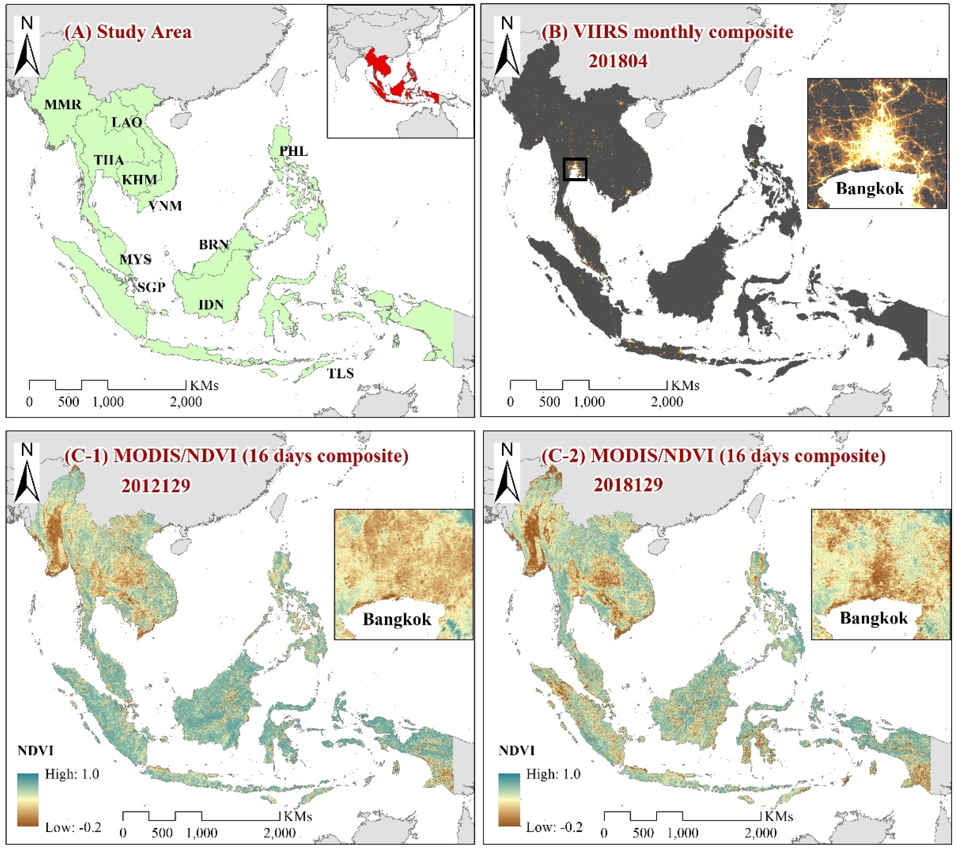
The study area is the Southeast Asia (SEA) region and contains 11 countries, including Brunei, Indonesia, Cambodia, Laos, Myanmar, Malaysia, Philippines, Singapore, Thailand, Timor-Leste, and Vietnam (Figure 1, Table 1). The SEA region covers an area of 448.25 × 10⁴ km2, with an estimated population of 648.69 million in 2017, which is the one of the most densely populated areas in the world. Meanwhile, the SEA region is also the fastest urbanizing and most rapidly developing area in the world, with an annual average urban population growth of 2.52% and an annual average gross domestic product (GDP) growth rate of 4.59% during 2008–2017. The high-intensive economic activities and rapid human growth exert a great pressure on the vegetation cover. Meanwhile, the SEA region has a tropical climate where vegetation resources are abundant and have little seasonal changes, and it is an ideal place to research the correlation between human influence and vegetation cover change.
2.2. Materials
2.2.1. VIIRS/DNB Nighttime Lights Data
The VIIRS/DNB is carried on the Suomi National Polar-Orbiting Partnership (Suomi-NPP), and the National Oceanic and Atmospheric Administration (NOAA) provides the monthly composite products. The products are stored with 15 arc-second (about 500 m at the equator) geographic grids, and they span the globe from 75 N to 65 S latitude with 6 tiles. The unit of average radiance values for monthly products is nanoWatts/cm2/sr, and data accuracy reaches 8 decimal places. The averaging method was employed to generate the monthly products, and some noises can be filtered to exclude in advance, including stray light, lightning, and lunar illumination. Meanwhile, the cloud cover is also removed by VIIRS Cloud Mask (VCM) products. Unfortunately, it is still impossible for several areas to get single good-quality coverage during that month due to consistent cloud cover or solar illumination, which indicates that zero or negative values do not always means no lights observed [37]. The relevant files, with extension “cf_cvg”, are integer numbers of cloud-free observation days for monthly composite products, and they are used to crosscheck the data reliability [51]. Finally, 73 monthly images (from April 2012 to April 2018) of “vcm” version of VIIRS/DNB monthly composite are selected, including Tile 3 (75 N/60 E to 00 N/120 E) and Tile 6 (00 N/60 E to 65 S/120 E).
2.2.2. MODIS NDVI Data
The 463 m resolution 16-day NDVI products (MOD13A1, version 6) were obtained from the Level-1 and Atmosphere Archive & Distribution System (LAADS) Distributed Active Archive Center (DAAC), NASA (https://ladsweb.modaps.eosdis.nasa.gov/archive/allData, last accessed on 5 February 2021). This 16-day composite is retrieved from the daily imagery, and it uses the best available value for each pixel, with low cloud cover, low view angle, and the highest value. The NDVI values range from −1 to 1, and data accuracy can reach 4 decimal places. Larger positive means values (>0.2) probably indicate a larger proportion of vegetation cover, where 0.2–0.4 represents sparsely vegetated or non-vegetated areas, and 0.4–0.8 represents green vegetated areas. To keep more data for trend analysis of relative values, NDVI means values that were in the range from 0.2 to 0.8 were all preserved [43]. The MODIS/NDVI data also have the Reliability layers that record the no data, snow/ice, and cloudy grids with values of −1, 2, and 3, respectively, and they can be applied to extract the reliable grids. To cover the entire SEA region, 19 MODIS tiles are required: h26v06-v07, h27v06–v09, h28v06-v09, h29v06-v09, h30v07-v09, h31v09, and h32v09. Then, the 19 tiles are mosaicked into one imagery for a certain date and converted from sinusoidal projection to the WSG-84 geographical coordinate system, with a pixel size of 15-arc seconds by the nearest resampling method. Thus, the spatial resolution of VIIRS/DNB and MODIS/NDVI data is unified under the same coordinate system. Furthermore, little geometric deviations were removed to ensure that the centroid of corresponding grids for two images were matched properly. Meanwhile, to match the time range of the VIIRS/DNB data, dates from the period 7 April 2012 (2012097) to 24 April 2018 (2018113) are selected for MODIS/NDVI data, and data in this period are all available, including 140 scenes.
3. Method
3.1. Preprocessing
For VIIRS/DNB time series (VTS), the “cf_cvg” file was used to identify the number of clear observations. If the clear observation was zero, the corresponding data value was reassigned to the average value with clear observation (>0) in 6 neighboring dates (for beginning and ending, the size might be less than 6). If there was no clear observation in 6 neighborhoods, the data value was then set to zero. This ensured the same length of each VTS and the smoothness of the VTS. The same process was applied to the MODIS/NDVI time series (MTS) based on the Reliability layer. Meanwhile, if the values for a certain total VTS or MTS were all <0, that meant there was no light or no vegetation cover all the time and no need to conduct further analysis for these areas. Then, VTS and MTS were further smoothed using a Savitzky–Golay filter to reduce the remaining outliers with a maximum retention of raw data [52]. Although low-value outliers were removed, there were still several high-value outliers (spike), especially for the VTS, which is ephemeral [48]. Thus, the same 6-size neighborhoods were applied to remove these spikes by defining a standard deviation threshold, which was selected by repeated trials based on several randomly selected samples (Equation (1)). After removal of these outliers, the VTS and MTS can be used for further analysis.
where n is the set of the original 6-size neighborhoods in VTS or MTS and xn is the data value, and are the standard deviation and average value, card is the size of set n. m is the set of effective values in 6-size neighborhoods, and xm is the data value for set m. If the absolute difference between a certain value and average was larger than 5, the value would be redistributed as the average value of the other effective values.
3.2. Segmentation of Time Series
The temporal segmentation process in this study was mainly based on the proposed MODTrendr model [40] and DBEST model [50]. To apply the time series analysis at large scales, we integrated and simplified these two models with less parameters. The major process was as follows:
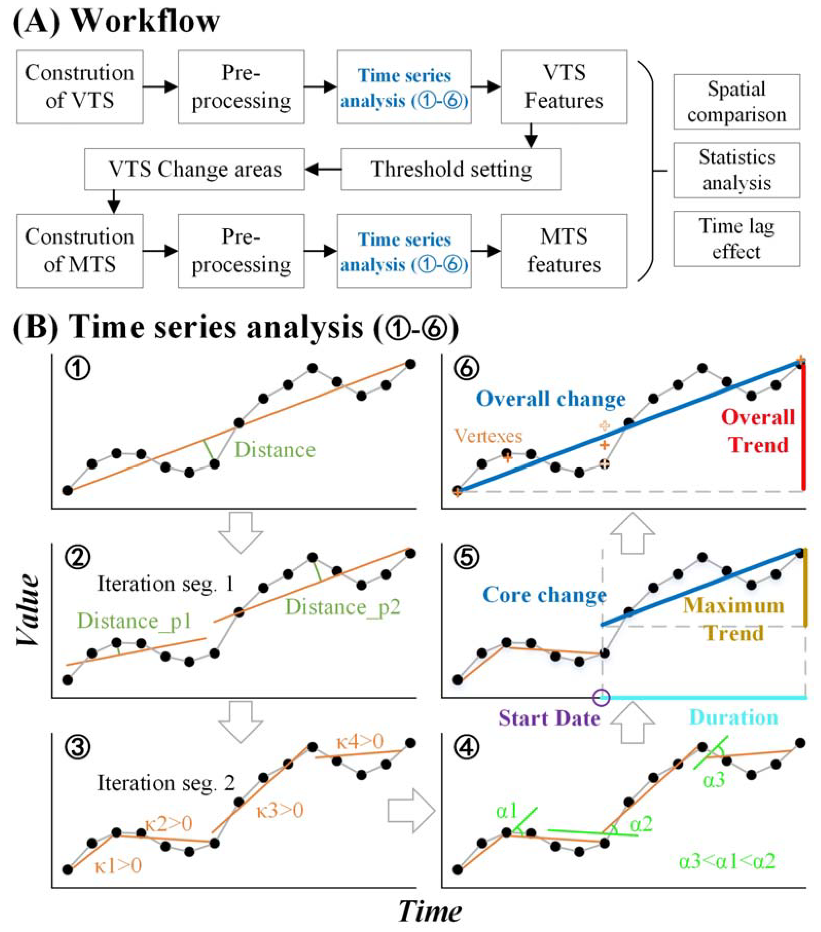
(1) A least squares first-order regression was conducted for the whole time series, where the date was digitized as 1-73 for VTS and 1-140 for MTS. Then, the perpendicular distance was calculated between each point and fitted line in Figure 2(B1).
(2) The point with the maximum distance to the fitted line was set as the potential turning points, and the turning points should also ensure that the period of the segmented time series is larger than 3 months. If the potential point did not satisfy this criterion, the point with the second or third largest distance was selected in Figure 2(B2).
(3) The time series could be divided into two parts by effective turning points. Notably, the valid turning points were the mutual nodes for the connected two sub time series.
(4) Then, the previous steps (1–3) were conducted for each part of the sub time series again in Figure 2(B3), and the iteration process was repeated 3 times for VTS and 4 times for MTS. That meant that the common maximum segments of VTS and MTS were 8 and 16, respectively.
(5) Moreover, the statistical significance test was conducted for each segment based on an F-statistic, with a significant level threshold of 0.05 [40,50]. The local segmentation would continue until statistical significance was detected.
The iteration number decided the number of turning points, and more turning points might reduce the residual sum but would result in over-fitting problems and large calculation complexity. When choosing the optimal turning point number, the Bayesian Information Criterion (BIC) was applied to segmentation results under different iteration numbers to minimize the BIC value [50,53]. After calculation for several samples, 3 and 4 were set as the optimal iteration number for VTS and MTS.
3.3. Incorporation and Feature Extraction
The segmentation would result in excess problems and the merge or incorporation should be applied for all the segments to simply the results. We used the sorted angle (included angles between adjoining fitted lines, [48]) method to composite each sub time series by a forward stepwise order in Figure 2(B4). Here, for the integration of both long-term sub time series (VTS > 24, MTS > 48, about 2 years), an incorporated process happened only when neighboring segments had the same change direction (sign of the change value, increment or decrement). For the composited new time series, the simple least square linear regression and significance test (0.05) was conducted again to get the new trend, until there were no more segment pairs that were satisfied with incorporation rules. In addition, once there was a new calculated trend, this iteration process started from the beginning to find the global minimum angle.
Once this merge process was finished, there were several new vertexes for segmented fitted lines, and the “Overall Trend” was fitted based on these vertexes. For middle vertexes, there might be two values for adjoining parts at one date, and the average value was reassigned. Meanwhile, for merge complement status, the segment with maximum absolute change value and same change direction with “Overall Trend” is set as the core change period in Figure 2(B6). To evaluate the time lag effect, 3 indexes of this core change period were calculated: “Maximum trend”, defined as the absolute change value of fitted line for the core change period; “Start date”, defined as occurrence date for the core change period; and “Duration”, defined as the duration time of the core change period in Figure 2(B5). That means, for a certain VTS or MTS, 4 main selected features are extracted to describe the features.
3.4. Time Lag Calculation and Validation
Considering the large areas in SEA, areas with large variation in human activities (V-change region) were first extracted based on the VTS overall trend, which could reduce the calculating amount and identify the target analysis area. A simple Gaussian fitted method was applied to identify the threshold of this kind of large variation of VTS [54]. Then, the vegetation cover trend was synchronously calculated in these V-change areas. Thus, the time lag effect (Lag_effect) and duration difference (Duration_diff) could be simply calculated by unifying the time range of these two time series (Equation (2)). The length was 143 for 16 day MTS, and it was unified into a time range of 70, which was the length of the VTS.
The validation for time series analysis had no mature scheme, and we conducted two parts according to the common validation schemes. For the NTL data, the other-source reference data were not common, and we randomly selected 300 grids with a large VIIRS/DNB trend, and 100 grids with a nearly zero VIIRS/DNB trend. The validation just focused on the segmentation and incorporation results for the time series itself by manual interpretation of the increasing and decreasing trends. Meanwhile, for vegetation cover, there were several other high spatial resolution diurnal data that could help validate the results. The randomly selected 300 grids were converted into polygon shapefiles and imported into Google Earth Engine. The NDVI from Landsat imageries in these polygons were calculated and the trend direction was compared with our MODIS/NDVI results.
3.5. Spatial Comparison and Pattern Analysis
Meanwhile, the Global Moran’s I index (−1 to 1) was introduced to evaluate the spatial distribution pattern of the above-mentioned time series features, where larger positive Moran’s I values indicated a more positive spatial distribution pattern and smaller negative Moran’s I values indicated a more negative spatial distribution pattern [55]. The Moran’s I index was first applied to the univariate overall trend, maximum trend, time lag effect, and duration difference. When evaluating the pattern of the relationship between the VIIRS and MODIS trend, a simple combination was conducted based on the quantization of the VTS and MTS trend level (Equation (3)). This grading could also help display and map the VIIRS and MODIS trend relation directly.
where a larger VII_MOD_level value indicates a greener trend (large MOD_index value) with less human impact increase (small VIIRS_index value).
All the above-mentioned processes were conducted by Python 3.6 and related libraries. Considering the similarity between the spatial distribution of the VIIRS/DNB and road network (Figure 1), we also conducted the pattern analysis with the distance to the present road networks by ArcMap 10.2. The road network data were acquired from the OpenStreetMap (https://download.geofabrik.de/asia.html, last accessed on 5 February 2021) by 2018.04. The major roads, including the motorway, trunk road, and primary road, were selected to evaluate the road influence on the VIIRS/DNB and MODIS/NDVI trends.
4. Results
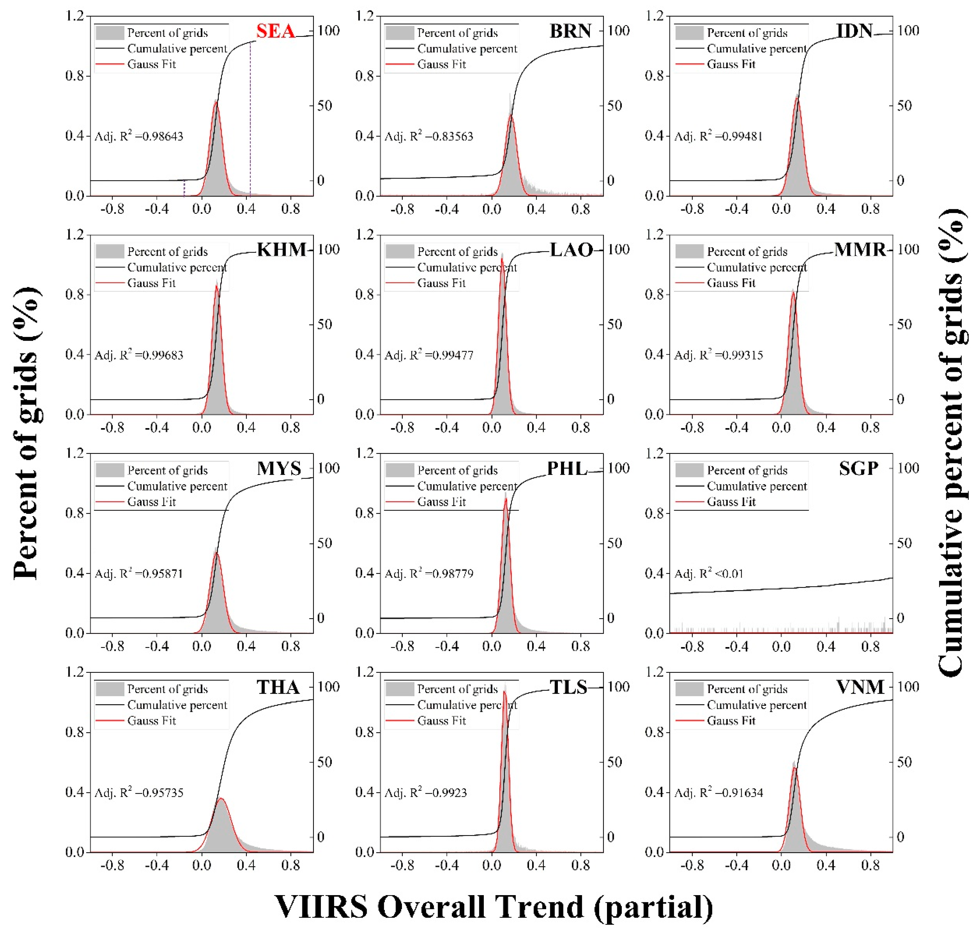
We conducted the statistics for the percent of grid counts under different overall VIIRS/DNB trend ranges (Figure 3). Ten of 11 SEA countries exhibited a typical Gaussian-shaped distribution, except for Singapore (SGP) with a small land area, which showed consistence with the existing research results [3,56]. Thus, we set the range (−0.2 to 0.4, peak areas of Gaussian curves) as the no VIIRS/DNB change area, and we set other regions (>0.4 or <−0.2) with large variation in human activities (V-change) as the target area for further analysis (Figure 3). About 1.85 × 10⁶ (8.64% of entire region) grids were extracted as V-change regions, with a maximum trend of statistical significance (0.05).
4.1. Human Activities Trend from VIIRS/DNB Time Series
The spatial distribution of the V-change regions mainly concentrated inside or around the big cities (Figure 4A), with a Moran’s I value of 0.535 (p < 0.01), which meant a strong positive spatial autocorrelation (Table 2). The magnitude of the overall VIIRS/DNB trend increment presented a radial shape descending from the city center. Meanwhile, there were still some VIIRS trend decreases around the big cities, such as the capital of Indonesia (IDN) and Brunei (BRN), mainly because of the urban renewal or construction of the ecological land according to the Google Earth historic imageries. Interestingly, a VIIRS/DNB increment could also be clearly observed along road networks (Figure 4A), which meant the construction of road or improvements of road lighting. According to the national statistics in Table 3, we could see that Singapore (SGP), BRN, Vietnam (VNM) and Malaysia (MYS) had the larger average overall VIIRS/DNB trend. These countries also had large GDP growth rate or urban population growth rate (Table 1). Apart from SGP, the large negative VIIRS/DNB trend also occurred in IDN, BRN, MYS, and VNM, which was mainly due to the balance between rural and urban population mobility [57].
The maximum VIIRS/DNB trend showed a similar spatial pattern with the overall VIIRS/DNB trend, with a Moran’s I of 0.420, and the scatter plot showed a strong linear relation between them (Figure 4B, Table 2). The average duration for the VIIRS/DNB core change period was about 48.04 months, where 39.95% had a duration over 60 months, indicating a continuous process of increased human activities (Figure 4C). Meanwhile, the occurrence of VIIRS/DNB change for about 74.73% of grids started at the benchmark month (2012.04), and the rest showed a relatively average distribution of the start month ranging from 1 to 65 (Figure 4C). Although the spatial distribution of this duration did not show an obvious pattern, but areas with longer duration tended to be located far away from the city center (Figure 4D).
4.2. Vegetation Cover Trend in V-Change Regions
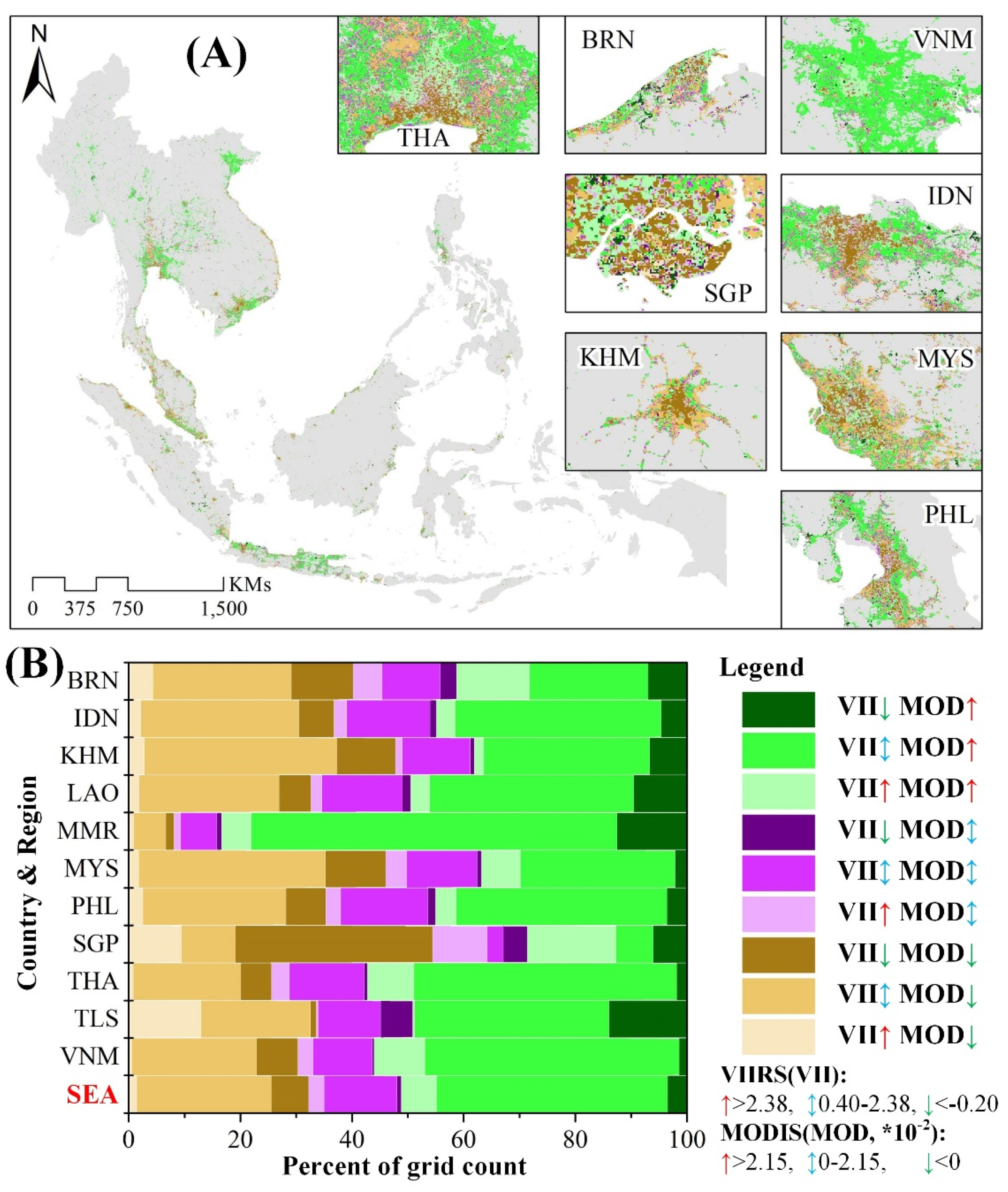
The same features of MODIS/NDVI time series were extracted based on V-change regions, where the maximum trend for all target grids shows statistical significance (0.05). According to statistics, the average value of the overall VIIRS/DNB trend for the SEA region was about 2.12, with a related MODIS/NDVI trend of 2.27 × 10⁻² (Table 3). That meant that although the human activities intensified in the SEA region, the vegetation cover still increased. Among all countries, Myanmar (MMR), VNM, and Thailand (THA) contributed the largest rate of vegetation cover increment. Only Cambodia (KHM) and SGP showed a decrease of vegetation cover both for total and positive VIIRS/DNB trend areas (Table 3). For negative VIIRS/DNB trend areas, the corresponding MODIS trend for all countries showed an increment, indicating the promotion of vegetation cover in areas with declining human activity (Table 3). For positive VIIRS/DNB trend areas, the average VIIRS/DNB trend for the SEA region rises to 2.38, while the related MODIS trend dropped to 2.15 × 10⁻². Thus, we set these two values as the threshold, combining with the above-mentioned V-change threshold, and each trend could be divided into three parts: VIIRS/DNB—high increase (>2.38), slight increase (0.40-2.38), decrease (<−0.20); MODIS/NDVI—high increase (>2.15 × 10⁻²), slight increase (0–2.15 × 10⁻²), decrease (<0). Thus, the composite of VIIRS/DNB trend and MODIS/NDVI trend could be divided into nine categories (Figure 5B).
For the spatial distribution of these nine categories, the “green” trends were observed to concentrate in THA, Laos (LAO), KHM, and IDN, while the “brown” trends were mainly in THA, MYS, and IDN (Figure 5A). When away from the center of the residential areas, the human impacts showed a decreasing pattern with an increase of the vegetation cover change, both for positive and negative VIIRS trends (Figure 5A). Meanwhile, the “green” trend and human activities weakening also showed a certain spatial clustering, with a Moran’s I of 0.289 (Table 2). We could also observe that for each country, at least 50% of grids underwent the process of vegetation cover increase or stabilize (green and purple part in Figure 5B), where more than 30% underwent a high increased (>2.15 × 10⁻²). Amongst them, MMR and Timor-Leste (TLS) had the highest proportion of grids to undergo the green process. For the whole region, most areas (≈41.42%) were under the slight VIIRS/DNB increase and high MODIS/NDVI increase, and even 6.32% of the area went “green” with heavy human activities increase (Figure 5B). Only about 1.46% went “brown” due to heavy human activities increase, and the rest (30.76%) of the “brown” areas had little human influence, where similar statistical conditions were also found for each country except SGP (Figure 5B).
4.3. Time Lag Effect of Vegetation Cover Response to Human Impacts
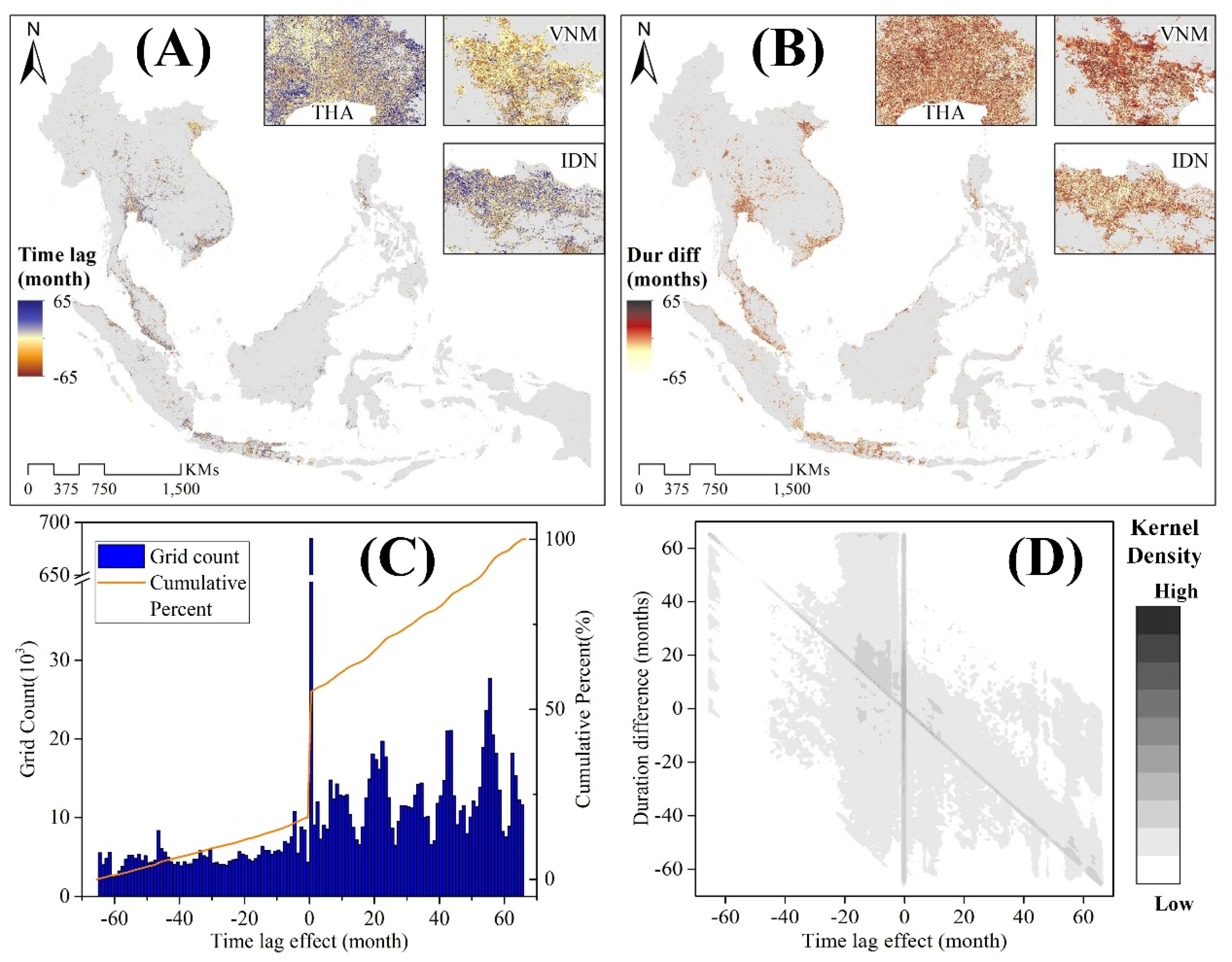
The time lag effect was obvious between the VIIRS/DNB and MODIS/NDVI trend in the SEA region, with an average of about 10.26 months (Table 4), comparing with 2-year time lag effect of non-human impacts [45]. This time lag effect could measure the feedback time of the vegetation cover change to the human activities. Meanwhile, the average duration of the MODIS trend was about 9 months shorter than that of the VIIRS/DNB trend for SEA region (Table 4). The spatial distribution of the time lag effect also showed a less regular pattern, with a Moran’s I value close to 0, but areas closer to cities were more likely to have a smaller time lag effect (Figure 6A, Table 2). That meant more populated area tended to have faster responses to the human activities and ecological degradation. Amongst them, 37.10% of the grids had no time lag effect, and the start month of the MODIS trend for 44.79% of the grids were posterior to that of the VIIRS/DNB trend (Figure 6C). The spatial distribution of duration difference between the start month of VIIRS/DNB and MODIS/NDVI maximum trend showed a uniform pattern due to the limit of the study period (Figure 6B). We also conducted the bivariate kernel density analysis between the time lag effect and duration difference. The plot showed two straight lines with high kernel density: a line with zero lag effect and a line with a slope of negative one (Figure 6D). The sum value of the diagonal line was about zero, which represented the same end time (end of research time, 2018.04) and a large probability of these two trends ongoing. While the vertical line represented that although the start time of the VIIRS/DNB and MODIS/NDVI change was likely to be the same, the duration difference was various, and the MODIS/NDVI change was likely to have longer durations (Figure 6D).
4.4. Validation and Pattern Analysis
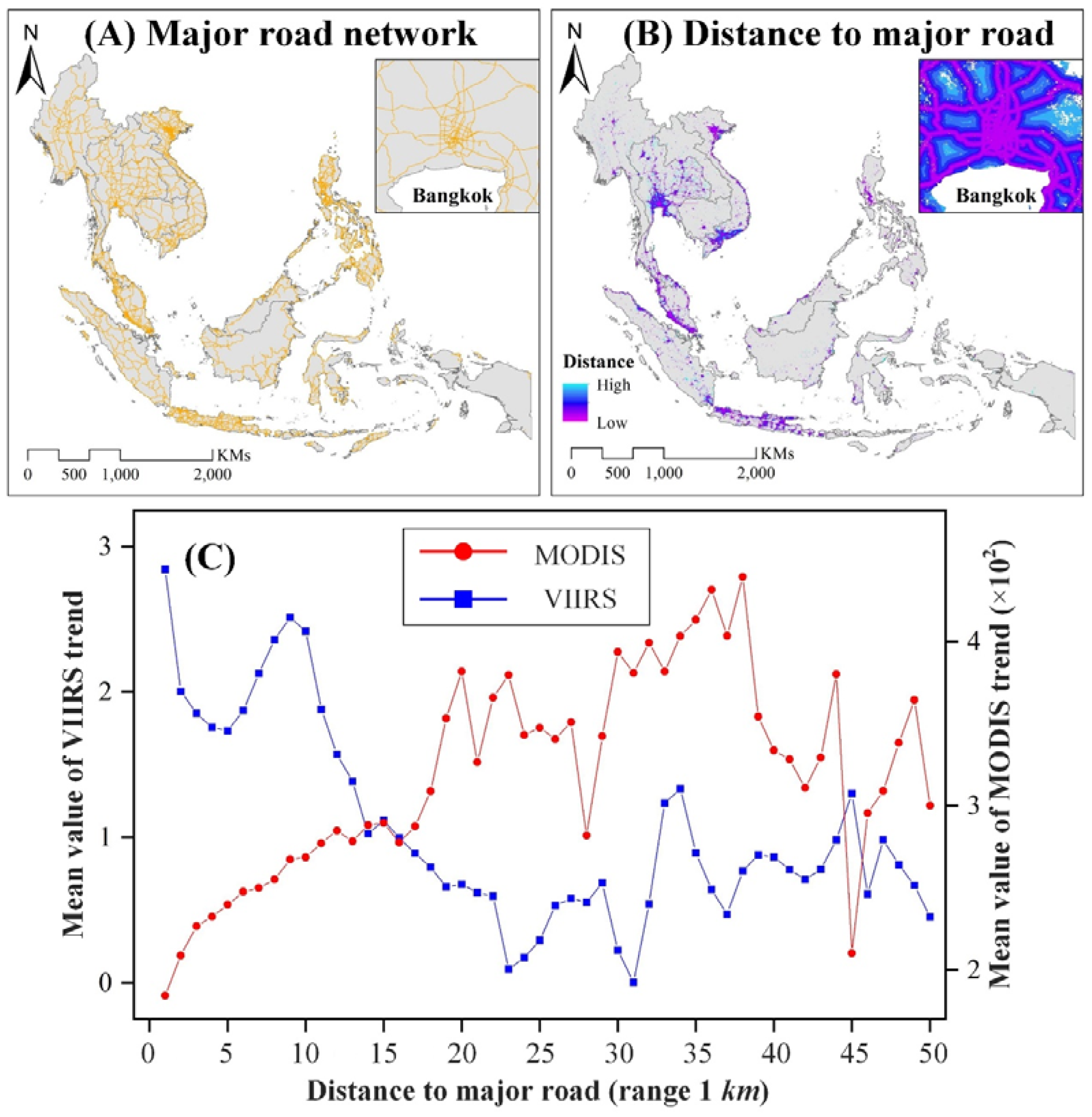
For NTL data, all 400 sites showed satisfied and reasonable results between manual interpretation and time series analysis. When comparing the MODIS NDVI trend of Landsat NDVI change, 300 samples also showed a full accordance in change directions and similar change magnitude, indicating the reliability of our proposed segmentation and incorporation method. Apart from samples, we also compared our results with other annual land cover products [58], and the difference by annual products showed a good accordance with our trend analysis. For pattern analysis, the V-change grids indeed showed a close relation with major road networks in SEA regions (Figure 7A,B). The average value of the VIIRS/DNB overall trend to the major roads exhibited a decrease when the distance to the major roads increased (Figure 7C). That meant areas closer to the major roads tended to have larger changes of human activities. For NDVI, the change rule was just the opposite, which meant that most of the green trend areas were far from the major roads (Figure 7C). This simple analysis also proved the correlation between the human impacts and vegetation cover change, where human activities along major roads were intensive and major roads could stimulate human activities change.
5. Discussion
5.1. Mapping Human Activities from Nighttime Lights
Mapping human activities is always a hot study issue, and there are several perspectives to map the human activities. Among all, the human mobility dataset, such as call detail records and social media data, can be the most accurate data source for the intuitive utility of geo-locations [59,60]. However, these kinds of data are hard to acquire for large scales due to some privacy policy, and huge amounts of data also make the processing extremely difficult. Alternatively, the open-access remote sensing dataset has naturally become the optimal choice to map long-term and large-scale human activities. Meanwhile, as a comprehensive problem, the human impact mapping should contain multiple factors, including population, infrastructure, and land cover. Thus, many human activities products are mostly based on multi-source diurnal data, such as terrestrial human footprint [3], Global Human Footprint [61], and Global Urban Footprint [62]. However, this integration process will bring some system errors, and unification of the temporal range and spatial resolution for all input data is sometimes tough. The NTL data can provide a reliable single indicator to represent the intensity of the human activities from the perspective of nocturnal activities [18,22], although the NTL intensity is not totally consistent with real human activities in some rural or urban-fringe areas [35,63]. Meanwhile, the trend analysis of NTL data can also provide some potential for further analysis. For example, the positive and negative VIIRS/DNB trend can be seen as an indicator to evaluate the magnitude of urban–rural population mobility or land-use conversion [64].
5.2. Human Impacts on Vegetation Cover Changes
Understanding vegetation cover dynamics is essential for land surface systems, environment protection, and human daily life, and it is influenced by multiple human and non-human factors [11,31]. Human impacts, mainly the urban process, have directly converted vegetation land into urban land and inhibited vegetation growth [6]. Meanwhile, the “green” trends were also found due to promoting growth and policy changes [5,10,11]. NTL data can only detect partial human activities change, while other human activity forms cannot be detected, such as cut down and plantations [65,66]. Thus, the human impacts from NTL data in this study could be concluded as one kind of representation index for the urbanization process, not for all the human activities. According to our study results, the green trends were found in the areas of the SEA region with increases in human activity (Table 3), indicating more attention to the human living environment in urban areas. This result was consistent with several recent mainstream findings, although the climatic factors are not considered in this study [10,11,12,13]. Thus, the simple assumption of the negative correlations between VIIRS/DNB nocturnal and MODIS/NDVI diurnal data seemed inappropriate. This result also reminded us of careful correlation analysis before data integration.
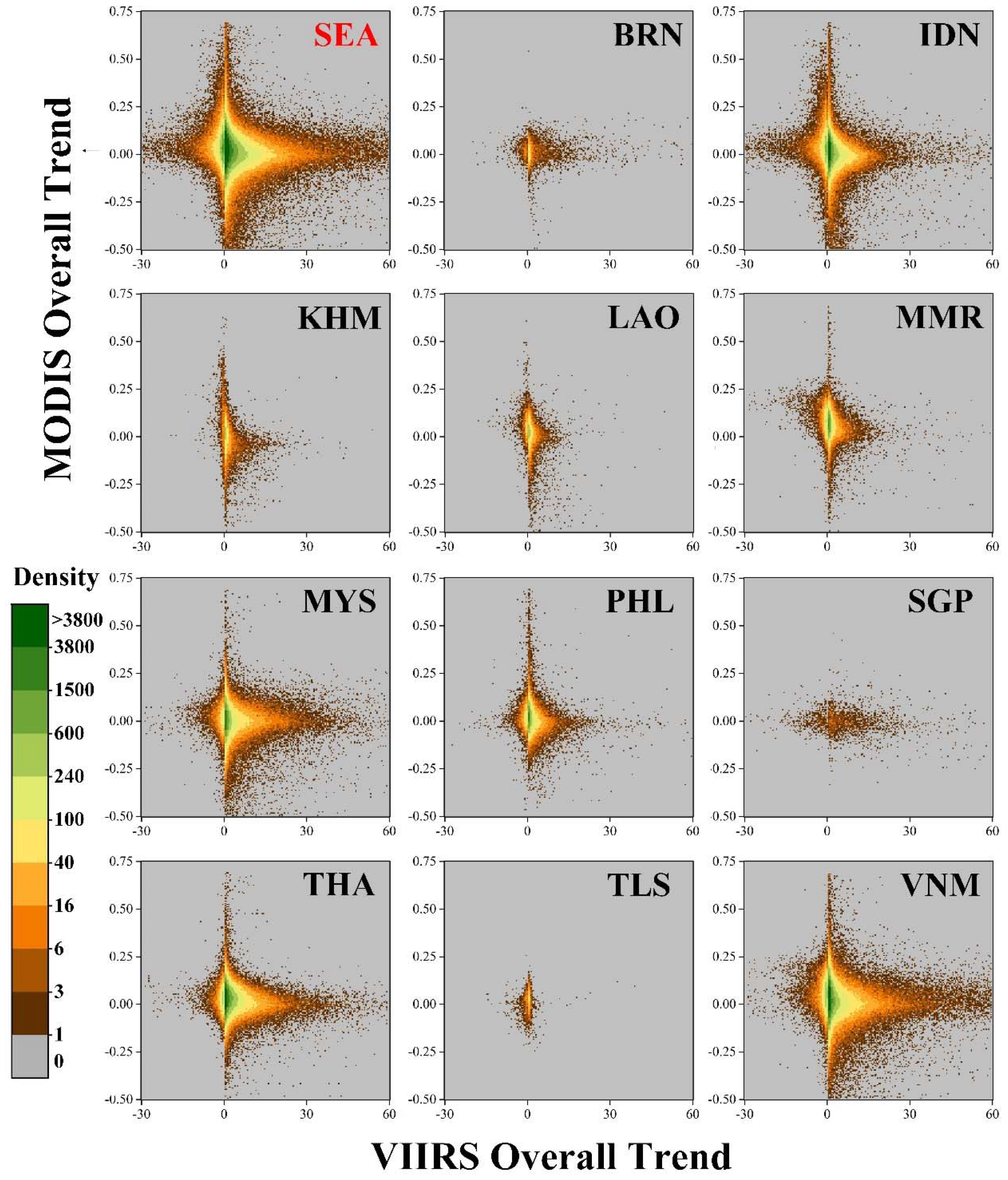
When comparing different combination of VIIRS trend and MODIS trend, the grid density heat map revealed a rhombus pattern for most countries and the whole SEA region, where the center has the highest grid density (Figure 8). For different countries, IDN, MYS, Philippines (PHL), THA, and VNM showed a more similar pattern with the whole region, while other countries showed a constrictive pattern due to little human activities change or small land area. For the whole region, the density distribution showed a symmetry both on the x-axis (VIIRS/DNB trend) and y-axis (MODIS trend), where negative VIIRS/DNB trend areas represented a tighter distribution (Figure 8). Meanwhile, this rhombus pattern had four obvious boundaries, and the trend value of both VIIRS/DNB and MODIS/NDVI were basically inside these boundaries (Figure 8). These boundaries could be seen as a reasonable and common balance between human activities and related vegetation cover change.
5.3. Influential Factors of Spatial Difference
Human impacts and vegetation cover change did not show an obvious spatial pattern (Figure 5A), but generally, “brown” trend areas were closer to the city center, where the city functions were intensive and there was little land for vegetation. For areas far from the center, there was enough land for ecological use even with heavy human impacts. For different countries, the “green” and “brown” trend difference can be attributed to multiple factors, such as economic structure, population changes, policy making, and climatic changes [10,11,67,68,69]. For example, THA had the highest green trend due to dependence on the agricultural economy, especially in urban and peri-urban areas [70]. The largest “brown areas” in THA and MYS were mainly due to a high urbanization rate, population growth rate, and economic development (Table 1). For the time lag effect, we could see that SGP, MMR, and BRN had the least time lag effect (Table 3), while for KHM, LAO, and THA, the vegetation response time was larger than 12 months. Meanwhile, the duration difference was obvious in BRN and SGP, with a larger or nearly the same duration for the MODIS/NDVI trend than the VIIRS/DNB trend. A smaller time lag effect and larger duration for a MODIS/NDVI increase might indicate a better ecological and environmental adjusting ability to the human activities. Apart from the above-mentioned factors, different protection schemes or policies of vegetation and concepts of urban planning can also result in this difference [68,69]. For example, in SGP, the rooftop garden is popular and can make urban areas greener [71], and BRN and SGP always have the high-level rate of urban forest cover with little construction in recent years.
5.4. Evaluation and Validation of Time Series Analysis
For a certain time series, the trend, occurrence date, and duration are the most important and core features. The temporal segmentation is the efficient feature extraction method for time series analysis, but it also brings some user-defined parameters or thresholds. Different artificial settings and choices will greatly influence the results, and lacking efficient reference data will magnify this problem. The proposed temporal segmentation method in this study needed less input parameters by omitting some steps of the DBEST and MODTrendr algorithms. By comparison with the same samples, it improved the calculation efficiency by reducing about 2/3 of the calculation time, also with good performance. There were also several other means to enhance the accuracy of trend analysis; for example, the object-based time series analysis was recently developed to take full advantage of imagery spatial and texture information [36,72]. However, for medium and low spatial resolution data, texture information and geographical object size are not enough for image segmentation. Thus, the pixel-based time series analysis was still the optimal scheme for VIIRS/DNB and MODIS/NDVI data. The validation of the time series analysis results was also a hard problem for time series analysis, and few studies gave the efficient validation schemes. The simple subtraction validation was sometimes contrary to the original idea of time series analysis, and the efficient validation could only be based on the qualitative assessment of the preselected reference data [73]. Thus, although our results showed a good performance with manual interpretation, our results were still the experimental consequence without rigorous validation, and they should be checked by more field data.
6. Conclusions
The negative and positive correlations between human impacts and vegetation cover are being widely discussed: the occupation of some ecological green land versus promotion of the vegetation cover by the ecological awareness and technology. Thus, Southeast Asia (SEA), with a rapid population and GDP increment, was selected to test this assumption over the last 7 years (2012–2018). The VIIRS/DNB NTL time series represented the change of human activities, and the MODIS/NDVI time series represented the vegetation cover change. The modified temporal segmentation was introduced to analyze and extract the features of these two sets of time series, including the overall trend and maximum trend, start date, and duration for the core change period. The Gaussian fitted model was first used to extract regions with large variation (VIIRS overall trend <−0.2 or >0.4) in human activities (V-change region) as the target analysis areas, about 1.85×10⁶ grids and 8.64% of the entire SEA. The spatial comparisons revealed that the average VIIRS/DNB overall trend was about 2.12 in the SEA V-change region, with an average MODIS/NDVI trend of 2.27 × 10⁻², indicating a slight green trend under the human impacts increment. When away from the center of residential areas, the human impacts showed a decreasing pattern with an increase of vegetation cover change. Meanwhile, the time lag effect was also discovered between the VIIRS/DNB and MODIS/NDVI trend, with an average of about 10.26 months, although the average duration of the MODIS trend was about 9 months shorter.
The results reveal the correlation between the human impacts and vegetation cover, and they can provide guidelines for the integration of similar datasets. However, there are still some points that deserve improving for this study. The results in this study only focused on the absolute trend value in a relatively short period. The DMSP (1992–2013) NTL data can be integrated to conduct a longer trend analysis, and other kinds of data can also be combined to improve the accuracy of the human impacts estimation, such as social media datasets. Meanwhile, the driving forces behind these changes should be evaluated, such as climatic changes, socioeconomic influences, and the vegetation management policy. Furthermore, although the vegetation cover changes were limited in areas with great change in human activities, the influence of non-human factors should also be removed to reduce the error. Moreover, the temporal segmentation, incorporation, and validation method at finer scales could also be promoted.
Author Contributions
Conceptualization, N.X. and M.L.; methodology, L.C.; formal analysis, N.X.; writing—original draft, N.X. and M.L.; writing—review and editing, N.X. and L.C.; visualization, N.X. and M.L.; supervision, M.L.; project administration, L.C. and M.L. All authors have read and agreed to the published version of the manuscript.
Funding
This work is funded by the National Key Research and Development Program of China (2017YFB0504205), the National Natural Science Foundation of China (41622109) and China postdoctoral Science foundation (2020M681545).
Institutional Review Board Statement
Not applicable.
Informed Consent Statement
Not applicable.
Data Availability Statement
The data presented in this study are available on request from the corresponding author. The data are not publicly available due to privacy.
Conflicts of Interest
The authors declare no conflict of interest.
References
- Zahid, H.J.; Robinson, E.; Kelly, R.L. Agriculture, population growth, and statistical analysis of the radiocarbon record. Proc. Natl. Acad. Sci. USA 2016, 113, 931–935. [Google Scholar] [CrossRef] [PubMed] [Green Version]
- United Nations Department of Economic and Social Affairs, Population Division. World Population Prospects: The 2017 Revision; United Nations Publications: New York, NY, USA, 2017. [Google Scholar]
- Venter, O.; Sanderson, E.W.; Magrach, A.; Allan, J.R.; Beher, J.; Jones, K.R.; Possingham, H.P.; Laurance, W.F.; Wood, P.; Fekete, B.M.; et al. Sixteen years of change in the global terrestrial human footprint and implications for bio-diversity conservation. Nat. Commun. 2016, 7, 12558. [Google Scholar] [CrossRef] [PubMed] [Green Version]
- Chi, G.Q.; Ho, H.C. Population stress: A spatiotemporal analysis of population change and land development at the county level in the contiguous United States, 2001–2011. Land Use Policy 2018, 70, 128–137. [Google Scholar] [CrossRef]
- Jia, W.X.; Zhao, S.Q.; Liu, S.G. Vegetation growth enhancement in urban environments of the Conterminous United States. Glob. Chang. Biol. 2018, 24, 4084–4094. [Google Scholar] [CrossRef] [PubMed]
- Hansen, M.C.; Potapov, P.V.; Moore, R.; Hancher, M.; Turubanova, S.A.; Tyukavina, A.; Thau, D.; Stehman, S.V.; Goetz, S.J.; Loveland, T.R.; et al. High-Resolution Global Maps of 21st-Century Forest Cover Change. Science 2013, 342, 850–853. [Google Scholar] [CrossRef] [Green Version]
- He, C.Y.; Gao, B.; Huang, Q.X.; Ma, Q.; Dou, Y.Y. Environmental degradation in the urban areas of China: Evidence from multi-source remote sensing data. Remote Sens. Environ. 2017, 193, 65–75. [Google Scholar] [CrossRef]
- Costanza, R.; De Groot, R.; Sutton, P.; van der Ploeg, S.; Anderson, S.J.; Kubiszewski, I.; Farber, S.; Turner, R.K. Changes in the global value of ecosystem services. Glob. Environ. Chang. 2014, 26, 152–158. [Google Scholar] [CrossRef]
- Newbold, T.; Hudson, L.N.; Day, J.; De Palma, A.; Díaz, S.; Echeverria-Londoño, S.; Edgar, M.J.; Feldman, A.; Garon, M.; Harrison, M.L.K.; et al. Global effects of land use on local terrestrial biodiversity. Nature 2015, 520, 45–50. [Google Scholar] [CrossRef] [PubMed] [Green Version]
- Zhang, Y.L.; Song, C.H.; Band, L.E.; Sun, G.; Li, J.X. Reanalysis of global terrestrial vegetation trends from MODIS products: Browning or greening? Remote Sens. Environ. 2017, 191, 145–155. [Google Scholar] [CrossRef] [Green Version]
- Zhao, S.Q.; Liu, S.G.; Zhou, D.C. Prevalent Vegetation Growth Enhancement in Urban Environment. Proc. Natl. Acad. Sci. USA 2016, 113, 6313–6318. [Google Scholar] [CrossRef] [Green Version]
- Huang, H.B.; Chen, Y.L.; Clinton, N.; Wang, J.; Wang, X.Y.; Liu, C.X.; Gong, P.; Yang, J.; Bai, Y.Q.; Zheng, Y.M.; et al. Mapping major land cover dynamics in Beijing using all Landsat images in Google Earth Engine. Remote Sens. Environ. 2017, 202, 166–176. [Google Scholar] [CrossRef]
- Zhang, X.Q.; Lei, Y.C.; Pang, Y.; Liu, X.Z.; Wang, J.Z. Tree mortality in response to climate change induced drought across Beijing, China. Clim. Chang. 2014, 124, 179–190. [Google Scholar] [CrossRef]
- Gong, P. Remote sensing of environmental change over China: A review. Chin. Sci. Bull. 2012, 57, 2793–2801. [Google Scholar] [CrossRef] [Green Version]
- Pei, F.S.; Li, X.; Liu, X.P.; Wang, S.J.; He, Z.J. Assessing the differences in net primary productivity between pre- and post-urban land development in China. Agric. For. Meteorol. 2013, 171, 174–186. [Google Scholar] [CrossRef]
- Yang, F.; Matsushita, B.; Yang, W.; Fukushima, T. Mapping the human footprint from satellite measurements in Japan. ISPRS J. Photogramm. Remote Sens. 2014, 88, 80–90. [Google Scholar] [CrossRef] [Green Version]
- Small, C.; Pozzi, F.; Elvidge, C.D. Spatial analysis of global urban extent from DMSP-OLS night lights. Remote Sens. Environ. 2005, 96, 277–291. [Google Scholar] [CrossRef]
- Elvidge, C.D.; Ziskin, D.; Baugh, K.E.; Tuttle, B.T.; Ghosh, T.; Pack, D.W.; Erwin, E.H.; Zhizhin, M. A Fifteen Year Record of Global Natural Gas Flaring Derived from Satellite Data. Energies 2009, 2, 595–622. [Google Scholar] [CrossRef]
- Elvidge, C.D.; Ghosh, T.; Hsu, F.C.; Zhizhin, M.; Bazilian, M. The Dimming of Lights in China during the COVID-19 Pan-demic. Remote Sens. 2020, 12, 2851. [Google Scholar] [CrossRef]
- Hu, K.; Qi, K.L.; Guan, Q.F.; Wu, C.Q.; Yu, J.M.; Qing, Y.X.; Zheng, J.; Wu, H.Y.; Li, X. A Scientometric Visualization Analysis for Night-Time Light Remote Sensing Research from 1991 to 2016. Remote Sens. 2017, 9, 802. [Google Scholar] [CrossRef] [Green Version]
- Huang, Q.X.; Yang, X.; Gao, B.; Yang, Y.; Zhao, Y.Y. Application of DMSP/OLS Nighttime Light Images: A Meta-Analysis and a Systematic Literature Review. Remote Sens. 2014, 6, 6844–6866. [Google Scholar] [CrossRef] [Green Version]
- Bennett, M.M.; Smith, L.C. Advances in using multitemporal night-time lights satellite imagery to detect, estimate, and monitor socioeconomic dynamics. Remote Sens. Environ. 2017, 192, 176–197. [Google Scholar] [CrossRef]
- Ma, T.; Zhou, C.H.; Pei, T.; Haynie, S.; Fan, J.F. Quantitative estimation of urbanization dynamics using time series of DMSP/OLS nighttime light data: A comparative case study from China’s cities. Remote Sens. Environ. 2012, 124, 99–107. [Google Scholar] [CrossRef]
- Peng, J.; Hu, Y.N.; Liu, Y.X.; Ma, J.; Zhao, S.Q. A new approach for urban-rural fringe identification: Integrating impervious surface area and spatial continuous wavelet transform. Landsc. Urban. Plan. 2018, 175, 72–79. [Google Scholar] [CrossRef]
- Shi, K.F.; Yu, B.L.; Huang, Y.X.; Hu, Y.J.; Yin, B.; Chen, Z.Q.; Chen, L.J.; Wu, J.P. Evaluating the Ability of NPP-VIIRS Nighttime Light Data to Estimate the Gross Domestic Product and the Electric Power Consumption of China at Multiple Scales: A Comparison with DMSP-OLS Data. Remote Sens. 2014, 6, 1705–1724. [Google Scholar] [CrossRef] [Green Version]
- Coscieme, L.; Sutton, P.C.; Anderson, S.; Liu, Q.; Elvidge, C.D. Dark Times: Nighttime satellite imagery as a detector of re-gional disparity and the geography of conflict. Gisci. Remote Sens. 2017, 54, 118–139. [Google Scholar] [CrossRef]
- Levin, N. The impact of seasonal changes on observed nighttime brightness from 2014 to 2015 monthly VIIRS DNB composites. Remote Sens. Environ. 2017, 193, 150–164. [Google Scholar] [CrossRef]
- Schneider, A.; Friedl, M.A.; Potere, D. Mapping global urban areas using MODIS 500-m data: New methods and datasets based on ‘urban ecoregions’. Remote Sens. Environ. 2010, 114, 1733–1746. [Google Scholar] [CrossRef]
- Chen, J.; Chen, J.; Liao, A.P.; Cao, X.; Chen, L.J.; Chen, X.H.; He, C.Y.; Han, G.; Peng, S.; Lu, M.; et al. Global land cover mapping at 30m resolution: A POK-based operational approach. ISPRS J. Photogramm. Remote Sens. 2015, 103, 7–27. [Google Scholar] [CrossRef] [Green Version]
- Tian, F.; Fensholt, R.; Verbesselt, J.; Grogan, K.; Horion, S.; Wang, Y.J. Evaluating temporal consistency of long-term global NDVI datasets for trend analysis. Remote Sens. Environ. 2015, 163, 326–340. [Google Scholar] [CrossRef]
- Miao, C.Y.; Yang, L.; Chen, X.H.; Gao, Y. The vegetation cover dynamics (1982-2006) in different erosion regions of the Yellow River Basin, China. Land Degrad. Dev. 2012, 23, 62–71. [Google Scholar] [CrossRef]
- Liu, Y.; Li, Y.; Li, S.C.; Motesharrei, S.C. Spatial and Temporal Patterns of Global NDVI Trends: Correlations with Climate and Human Factors. Remote Sens. 2015, 7, 13233–13250. [Google Scholar] [CrossRef] [Green Version]
- Jing, W.L.; Yang, Y.P.; Yue, X.F.; Zhao, X.D. Mapping Urban Areas with Integration of DMSP/OLS Nighttime Light and MODIS Data Using Machine Learning Techniques. Remote Sens. 2015, 7, 12419–12439. [Google Scholar] [CrossRef] [Green Version]
- Sharma, R.C.; Tateishi, R.; Hara, K.; Gharechelou, S.; Iizuka, K. Global mapping of urban built-up areas of year 2014 by combining MODIS multispectral data with VIIRS nighttime light data. Int. J. Digit. Earth 2016, 9, 1004–1020. [Google Scholar] [CrossRef]
- Goldblatt, R.; Stuhlmacher, M.F.; Tellman, B.; Clinton, N.; Hanson, G.; Georgescu, M.; Wang, C.Y.; Serrano-Candela, F.; Khandelwal, A.K.; Cheng, W.H.; et al. Using Landsat and nighttime lights for supervised pixel-based image classification of urban land cover. Remote Sens. Environ. 2018, 205, 253–275. [Google Scholar] [CrossRef]
- Silveira, E.M.D.O.; Bueno, I.T.; Junior, F.W.A.; De Mello, J.M.; Scolforo, J.R.S.; Wulder, M.A. Using Spatial Features to Reduce the Impact of Seasonality for Detecting Tropical Forest Changes from Landsat Time Series. Remote Sens. 2018, 10, 808. [Google Scholar] [CrossRef] [Green Version]
- National Centers for Environment Information (NCEI), National Oceanic and Atmospheric Administration (NOAA). Available online: http://www.ngdc.noaa.gov/eog/viirs/download_monthly.html (accessed on 1 July 2018).
- Fensholt, R.; Proud, S.R. Evaluation of Earth Observation based global long term vegetation trends—Comparing GIMMS and MODIS global NDVI time series. Remote Sens. Environ. 2012, 119, 131–147. [Google Scholar] [CrossRef]
- Yin, H.; Prishchepov, A.V.; Kuemmerle, T.; Bleyhl, B.; Buchner, J.; Radeloff, V.C. Mapping agricultural land abandonment from spatial and temporal segmentation of Landsat time series. Remote Sens. Environ. 2018, 210, 12–24. [Google Scholar] [CrossRef]
- Sulla-Menashe, D.; Kennedy, R.E.; Yang, Z.Q.; Braaten, J.; Krankina, O.N.; Friedl, M.A. Detecting forest disturbance in the Pacific Northwest from MODIS time series using temporal segmentation. Remote Sens. Environ. 2014, 151, 114–123. [Google Scholar] [CrossRef]
- Roman, M.O.; Stokes, E.C. Holidays in lights: Tracking cultural patterns in demand for energy services. Earth’s Future 2015, 3, 182–205. [Google Scholar] [CrossRef]
- Eklundh, L.; Olsson, L. Vegetation index trends for the African Sahel 1982–1999. Geophys. Res. Lett. 2003, 30, 30. [Google Scholar] [CrossRef]
- Jamali, S.; Seaquist, J.; Eklundh, L.; Ardö, J. Automated mapping of vegetation trends with polynomials using NDVI imagery over the Sahel. Remote Sens. Environ. 2014, 141, 79–89. [Google Scholar] [CrossRef]
- Nguyen, T.H.; Jones, S.D.; Soto-Berelov, M.; Haywood, A.; Hislop, S. A spatial and temporal analysis of forest dynamics using Landsat time-series. Remote Sens. Environ. 2018, 217, 461–475. [Google Scholar] [CrossRef]
- Wu, D.H.; Zhao, X.; Liang, S.L.; Zhou, T.; Huang, K.C.; Tang, B.J.; Zhao, W.Q. Time-lag effects of global vegetation responses to climate change. Glob. Chang. Biol. 2015, 21, 3520–3531. [Google Scholar] [CrossRef] [PubMed]
- Niță, M.-D.; Munteanu, C.; Gutman, G.; Abrudan, I.V.; Radeloff, V.C. Widespread forest cutting in the aftermath of World War II captured by broad-scale historical Corona spy satellite photography. Remote Sens. Environ. 2018, 204, 322–332. [Google Scholar] [CrossRef]
- Bürgi, M.; Östlund, L.; Mladenoff, D.J. Legacy Effects of Human Land Use: Ecosystems as Time-Lagged Systems. Ecosystems 2017, 20, 94–103. [Google Scholar] [CrossRef] [Green Version]
- Kennedy, R.E.; Yang, Z.G.; Cohen, W.B. Detecting trends in forest disturbance and recovery using yearly Landsat time series: 1. LandTrendr—Temporal segmentation algorithms. Remote Sens. Environ. 2010, 114, 2897–2910. [Google Scholar] [CrossRef]
- Verbesselt, J.; Hyndman, R.; Newnham, G.; Culvenor, D. Detecting trend and seasonal changes in satellite image time series. Remote Sens. Environ. 2010, 114, 106–115. [Google Scholar] [CrossRef]
- Jamali, S.; Jönsson, P.; Eklundh, L.; Ardö, J.; Seaquist, J. Detecting changes in vegetation trends using time series segmentation. Remote Sens. Environ. 2015, 156, 182–195. [Google Scholar] [CrossRef]
- Wang, R.; Wan, B.; Guo, Q.H.; Hu, M.S.; Zhou, S.P. Mapping Regional Urban Extent Using NPP-VIIRS DNB and MODIS NDVI Data. Remote Sens. 2017, 9, 862. [Google Scholar] [CrossRef] [Green Version]
- Chen, J.; Jonsson, P.; Tamura, M.; Gu, Z.H.; Matsushita, B.; Eklundh, L. A simple method for reconstructing a high-quality NDVI time-series data set based on the Savitzky-Golay filter. Remote Sens. Environ. 2004, 91, 332–344. [Google Scholar] [CrossRef]
- Schwarz, G.E. Estimating the dimension of a model. Ann. Stat. 1978, 6, 461–464. [Google Scholar] [CrossRef]
- Abrahams, A.; Oram, C.; Lozano-Gracia, N. Deblurring DMSP nighttime lights: A new method using Gaussian filters and frequencies of illumination. Remote Sens. Environ. 2018, 210, 242–258. [Google Scholar] [CrossRef]
- Tiefelsdorf, M. The saddlepoint approximation of Moran’s I’s and local Moran’s I-i’s reference distributions and their numerical evaluation. Geogr. Anal. 2002, 34, 187–206. [Google Scholar] [CrossRef]
- Wang, J.; Lin, Y.F.; Zhai, T.L.; He, T.; Qi, Y.; Jin, Z.F.; Cai, Y.M. The role of human activity in decreasing ecologically sound land use in China. Land Degrad. Dev. 2018, 29, 446–460. [Google Scholar] [CrossRef]
- Han, B.L.; Wang, R.S.; Tao, Y.; Gao, H. Urban population agglomeration in view of complex ecological niche: A case study on Chinese prefecture cities. Ecol. Indic. 2014, 47, 128–136. [Google Scholar] [CrossRef]
- Miettinen, J.; Shi, C.H.; Liew, S.C. 2015 Land cover map of Southeast Asia at 250 m spatial resolution. Remote Sens. Lett. 2016, 7, 701–710. [Google Scholar] [CrossRef]
- Deville, P.; Linard, C.; Martin, S.; Gilbert, M.; Stevens, F.R.; Gaughan, A.E.; Blondel, V.D.; Tatem, A.J. Dynamic population mapping using mobile phone data. Proc. Natl. Acad. Sci. USA 2014, 111, 15888–15893. [Google Scholar] [CrossRef] [PubMed] [Green Version]
- Ma, T. Multi-Level Relationships between Satellite-Derived Nighttime Lighting Signals and Social Media–Derived Human Population Dynamics. Remote Sens. 2018, 10, 1128. [Google Scholar] [CrossRef] [Green Version]
- Wildlife Conservation Society (WCS) and Center for International Earth Science Information Network (CIESIN), NASA So-cioeconomic Data and Applications Center (SEDAC). Last of the Wild Project, Version 2, 2005 (LWP-2): Global Human Footprint Dataset (Geographic). Available online: http://http://sedac.ciesin.columbia.edu/data/collection/wildareas-v2 (accessed on 26 September 2018).
- Esch, T.; Heldens, W.; Hirner, A.; Keil, M.; Marconcini, M.; Roth, A.; Zeidler, J.; Dech, S.; Strano, E. Breaking new ground in mapping human settlements from space—The Global Urban Footprint. ISPRS J. Photogramm. Remote Sens. 2017, 134, 30–42. [Google Scholar] [CrossRef] [Green Version]
- Zhang, Q.; Wang, P.; Chen, H.; Huang, Q.L.; Jiang, H.B.; Zhang, Z.J.; Zhang, Y.M.; Luo, X.; Sun, S.J. A novel method for urban area extraction from VIIRS DNB and MODIS NDVI data: A case study of Chinese cities. Int. J. Remote Sens. 2017, 38, 6094–6109. [Google Scholar] [CrossRef]
- Chen, R.S.; Ye, C.; Cai, Y.L.; Xing, X.S.; Chen, Q. The impact of rural out-migration on land use transition in China: Past, present and trend. Land Use Policy 2014, 40, 101–110. [Google Scholar] [CrossRef]
- Van der Werf, G.R.; Dempewolf, J.; Trigg, S.N.; Randerson, J.T.; Kasibhatla, P.S.; Giglio, L.; Murdiyarso, D.; Peters, W.; Morton, D.C.; Collatz, G.J.; et al. Climate regulation of fire emissions and deforestation in equatorial Asia. Proc. Natl. Acad. Sci. USA 2008, 105, 20350–20355. [Google Scholar] [CrossRef] [Green Version]
- Carlson, K.M.; Curran, L.M.; Ratnasari, D.; Pittman, A.M.; Soares-Filho, B.S.; Asner, G.P.; Trigg, S.N.; Gaveau, D.A.; Lawrence, D.; Rodrigues, H.O. Committed carbon emissions, deforestation, and community land conversion from oil palm plantation expansion in West Kalimantan, Indonesia. Proc. Natl. Acad. Sci. USA 2012, 109, 7559–7564. [Google Scholar] [CrossRef] [PubMed] [Green Version]
- Zhu, Z.C.; Piao, S.L.; Myneni, R.B.; Huang, M.T.; Zeng, Z.Z.; Canadell, J.G.; Ciais, P.; Sitch, S.; Friedlingstein, P.; Arneth, A.; et al. Greening of the Earth and its drivers. Nat. Clim. Chang. 2018, 6, 791–795. [Google Scholar] [CrossRef]
- Meng, Z.Q.; Liu, M.; Gao, C.C.; Zhang, Y.; She, Q.N.; Long, L.B.; Tu, Y.; Yang, Y.X. Greening and browning of the coastal areas in mainland China: Spatial heterogeneity, seasonal variation and its influential factors. Ecol. Indic. 2020, 110, 105888. [Google Scholar] [CrossRef]
- Shi, Y.; Jin, N.; Ma, X.L.; Wu, B.Y.; He, Q.S.; Yue, C.; Yu, Q. Attribution of climate and human activities to vegetation change in China using machine learning techniques. Agric. For. Meteorol. 2020, 294, 108146. [Google Scholar] [CrossRef]
- Vagneron, I. Economic appraisal of profitability and sustainability of peri-urban agriculture in Bangkok. Ecol. Econ. 2007, 61, 516–529. [Google Scholar] [CrossRef] [Green Version]
- Wong, N.H.; Chen, Y.; Ong, C.L.; Sia, A. Investigation of thermal benefits of rooftop garden in the tropical environment. Build. Environ. 2003, 38, 261–270. [Google Scholar] [CrossRef]
- Belgiu, M.; Csillik, O. Sentinel-2 cropland mapping using pixel-based and object-based time-weighted dynamic time warping analysis. Remote Sens. Environ. 2018, 204, 509–523. [Google Scholar] [CrossRef]
- Cohen, W.B.; Yang, Z.G.; Kennedy, R. Detecting trends in forest disturbance and recovery using yearly Landsat time series: 2. TimeSync—Tools for calibration and validation. Remote Sens. Environ. 2010, 114, 2911–2924. [Google Scholar] [CrossRef]
Figure 1.
(A) Study area of Southeast Asia, (B) original Visible Infrared Imaging Radiometer Suite - Day/Night Band (VIIRS/DNB) monthly composite data for 2018.04, and (C) 16 days composite of moderate resolution imaging spectroradiometer (MODIS)/normalized difference vegetation index (NDVI) data for 9 May 2012 (2012129) and 10 May 2018 (2018129).

Figure 2.
The workflow of this study (A), and the sketch map (B) for a VIIRS/DNB time series (VTS) and MODIS/NDVI time series (MTS) analysis, including temporal segmentation (B1–B3), iteration number of 2 as an example) and incorporation (B4—B6). Where “distance_” is the perpendicular distance between each data point and fitted line, “κ” is the slope of the fitted line, and “α” is the included angle between two adjoining fitted lines. The outputs of time series analysis contain four main features, including overall trend, maximum trend, start month, and duration.

Figure 3.
Frequency histogram shows the percent of all grid counts under different VIIRS/DNB overall trend ranges (trend interval: 0.01, partial not total, grid count: ≈21.41 × 10⁶), and the cumulative frequency curve shows the cumulative percent of grid counts for the whole Southeast Asia (SEA) region and 11 countries. The Gaussian fit curve shows the fitted distribution of the VIIRS change.

Figure 4.
The spatial distribution of the (A) VIIRS/DNB overall trend and (D) duration of the maximum trend (M_Tr). The statistics also show (B) relations between VIIRS/DNB overall trend and maximum trend, and (C) histogram of M_Tr duration and cumulative frequency of start month for M_Tr for SEA region for VIIRS change areas (grids count: ≈1.85 × 10⁶).

Figure 5.
The spatial pattern (A) and statistics (B) between VIIRS/DNB overall trend and MODIS/NDVI overall trend for the whole Southeast Asia region (SEA, grids count: ≈1.85 × 10⁶) and 11 countries. The color bar (B) shows the different proportion of grid density under different combinations of VIIRS/DNB and MODIS/NDVI change level.

Figure 6.
Spatial distribution of time lag effect (A) and duration difference (B) between MODIS/NDVI maximum trend and VIIRS/DNB maximum trend. The histogram and cumulative percent of grid count for time lag effect (C) and the bivariate kernel density between time lag effect and duration difference (D) for VIIRS change areas (grids count: ≈1.85 × 10⁶).

Figure 7.
The spatial distribution of a major road network from OpenStreetMap in the Southeast Asia (SEA) region (A) and distance from VIIRS change grids (grids count: ≈1.85 × 10⁶) to major roads (B). (C) Mean value of VIIRS/DNB and MODIS/NDVI overall trends under different distance (kilometers, KMs) to the nearest major roads.

Figure 8.
The heat map shows the correlation between VIIRS/DNB overall trend and MODIS/NDVI overall trend for the Southeast Asia region (SEA, total grids count: ≈1.85 × 10⁶) and 11 countries. The color map shows the different levels of grid density.
Figure 8.
The heat map shows the correlation between VIIRS/DNB overall trend and MODIS/NDVI overall trend for the Southeast Asia region (SEA, total grids count: ≈1.85 × 10⁶) and 11 countries. The color map shows the different levels of grid density.


Table 1.
The basic information for 11 countries in Southeast Asia (SEA), including name abbreviation (Abbr.), area, 2012 and 2018 population (pop), 2008–2017 annual growth rate (an_gr) of urban population (U-pop), 2008–2017 annual growth rate of rural population (R-pop), and 2008–2017 annual growth rate of gross domestic product (GDP). The data are collected from the DataBank of World Bank (https://data.worldbank.org.cn/ (accessed on 26 January 2021)).
| Country. | Abbr. | Area (104km2) | Pop_2012 (106) | Pop_2018 (106) | U-pop an_gr (%) | R-pop an_gr(%) | GDP an_gr (%) |
|---|---|---|---|---|---|---|---|
| Brunei | BRN | 0.58 | 0.40 | 0.43 | 1.79 | −0.62 | −0.26 |
| Indonesia | IDN | 190.11 | 248.45 | 267.66 | 2.65 | −0.21 | 5.46 |
| Cambodia | KHM | 18.25 | 14.78 | 16.25 | 3.26 | 1.12 | 6.24 |
| Laos | LAO | 23.11 | 6.44 | 7.06 | 3.36 | 0.54 | 7.67 |
| Myanmar | MMR | 67.26 | 51.41 | 53.71 | 1.50 | 0.54 | 7.90 |
| Malaysia | MYS | 33.15 | 29.07 | 31.53 | 2.71 | −0.82 | 4.74 |
| Philippines | PHL | 29.58 | 97.21 | 106.65 | 1.86 | 1.40 | 5.61 |
| Singapore | SGP | 0.07 | 5.31 | 5.64 | 2.01 | 0.00 | 4.41 |
| Thailand | THA | 51.62 | 67.84 | 69.43 | 2.50 | −1.25 | 3.05 |
| Timor-Leste | TLS | 1.50 | 1.13 | 1.27 | 3.20 | 1.48 | −0.38 |
| Vietnam | VNM | 33.02 | 89.80 | 95.54 | 3.18 | 0.08 | 6.01 |
Table 2.
Global Moran’s I index (G_MI) and z-score of seven indexes for 11 countries and SEA region, including VIIRS overall trend, VIIRS maximum trend, MODIS overall trend, MODIS maximum trend, VII_MOD_level, Time lag effect, and Duration difference. z-score > 2.58 indicates the 1% significance level.
| VIIRS_Overall | VIIRS_Max | MODIS_Overall | MODIS_Max | |||
|---|---|---|---|---|---|---|
| G_MI | 0.5351 | 0.4203 | 0.2342 | 0.1603 | ||
| z-score | 15,562.6845 | 12,219.3249 | 6796.0787 | 4651.3304 | ||
| VII_MOD_level * | Time lag effect | Duration_diff | ||||
| G_MI | 0.2886 | 0.0561 | 0.0602 | |||
| z-score | 8374.7861 | 1628.5557 | 1747.3804 | |||
* VII_MOD level was set according to Figure 5, for MODIS_index: >2.15 × 10⁻²→3, 0–2.15 × 10⁻²→2, <0→1; for VIIRS_index: >2.38→1, 0.40–2.38→2, <−0.20→3
Table 3.
The average VIIRS/DNB and MODIS/NDVI trend value under the all VIIRS overall trends, positive VIIRS overall trends (>0), and negative VIIRS overall trends (<0) for only VIIRS change areas (grids count: ≈1.85 × 10⁶). The cell background color shows the different levels of trend values, where a darker color indicates a larger absolute value.
| Regions | All VIIRS Trend | Positive VIIRS Trend | Negative VIIRS Trend | |||
|---|---|---|---|---|---|---|
| VIIRS | MOD (10−4) | VIIRS | MOD (10−4) | VIIRS | MOD (10−4) | |
| SEA | 2.12 | 226.85 | 2.38 | 215.34 | −2.11 | 417.66 |
| BRN | 3.90 | 109.34 | 4.88 | 93.09 | −1.97 | 207.52 |
| IDN | 1.21 | 146.72 | 1.58 | 125.66 | −3.08 | 390.76 |
| KHM | 1.41 | −13.58 | 1.65 | −109.77 | −0.78 | 834.16 |
| LAO | 1.07 | 140.45 | 1.38 | 73.06 | −1.02 | 597.85 |
| MMR | 0.87 | 673.79 | 1.20 | 643.01 | −1.13 | 857.61 |
| MYS | 2.62 | 26.36 | 2.85 | 20.09 | −1.86 | 153.10 |
| PHL | 1.32 | 184.38 | 1.52 | 179.26 | −1.21 | 247.37 |
| SGP | 7.23 | −42.50 | 10.59 | −64.47 | −6.38 | 46.67 |
| THA | 1.75 | 290.85 | 1.85 | 289.52 | −1.28 | 331.24 |
| TLS | 0.15 | 153.99 | 0.82 | 205.09 | −1.23 | 48.31 |
| VNM | 4.60 | 311.47 | 4.75 | 308.25 | −1.52 | 451.98 |
Table 4.
The start month and duration between core change period of VIIRS/DNB and MODIS/NDVI time series. The colored cells show the time lag effect of human impacts on vegetation cover change.
Table 4.
The start month and duration between core change period of VIIRS/DNB and MODIS/NDVI time series. The colored cells show the time lag effect of human impacts on vegetation cover change.
| Regions | Start Month (2012.04–2018.04) | Duration (Months) | |||
|---|---|---|---|---|---|
| VIIRS | MODIS | Lag Effect | VIIRS | MODIS | |
| SEA | 8.65 | 18.91 | 10.26 | 48.03 | 39.73 |
| BRN | 7.28 | 17.67 | 10.39 | 34.87 | 42.23 |
| IDN | 9.10 | 19.74 | 10.64 | 49.68 | 39.65 |
| KHM | 4.93 | 18.66 | 13.73 | 54.05 | 36.52 |
| LAO | 8.57 | 20.65 | 12.08 | 47.37 | 39.87 |
| MMR | 9.35 | 15.81 | 6.46 | 53.27 | 41.69 |
| MYS | 9.77 | 19.51 | 9.74 | 44.01 | 38.11 |
| PHL | 9.60 | 18.73 | 9.13 | 47.23 | 40.51 |
| SGP | 12.88 | 19.41 | 6.53 | 39.39 | 38.90 |
| THA | 7.73 | 19.95 | 12.22 | 46.14 | 38.96 |
| TLS | 7.41 | 17.34 | 9.93 | 50.28 | 43.73 |
| VNM | 8.38 | 16.18 | 7.80 | 49.71 | 41.59 |
Publisher’s Note: MDPI stays neutral with regard to jurisdictional claims in published maps and institutional affiliations. |
© 2021 by the authors. Licensee MDPI, Basel, Switzerland. This article is an open access article distributed under the terms and conditions of the Creative Commons Attribution (CC BY) license (http://creativecommons.org/licenses/by/4.0/).
Share and Cite
MDPI and ACS Style
Xia, N.; Li, M.; Cheng, L. Mapping Impacts of Human Activities from Nighttime Light on Vegetation Cover Changes in Southeast Asia. Land 2021, 10, 185. https://doi.org/10.3390/land10020185
AMA Style
Xia N, Li M, Cheng L. Mapping Impacts of Human Activities from Nighttime Light on Vegetation Cover Changes in Southeast Asia. Land. 2021; 10(2):185. https://doi.org/10.3390/land10020185
Chicago/Turabian StyleXia, Nan, Manchun Li, and Liang Cheng. 2021. "Mapping Impacts of Human Activities from Nighttime Light on Vegetation Cover Changes in Southeast Asia" Land 10, no. 2: 185. https://doi.org/10.3390/land10020185
Note that from the first issue of 2016, this journal uses article numbers instead of page numbers. See further details here.