Mesospheric Bore Observations Using Suomi-NPP VIIRS DNB during 2013–2017
by
 , ,
, ,
Yucheng Su
1,2,*, 
Jia Yue
2,
Xiao Liu
3,
Steven D. Miller
4 ,
,
William C. Straka III
5,
Steven M. Smith
6,
Dong Guo
1 and
Shengli Guo
1 1
Institute of Space Weather, Nanjing University of Information Science and Technology, Nanjing 210044, China
2
Center for Atmospheric Science, Hampton University, Hampton, VA 23668, USA
3
School of Mathematics and Information Science, Henan Normal University, Xinxiang 453000, China
4
Cooperative Institute for Research in the Atmosphere, Colorado State University, Fort Collins, CO 80523, USA
5
Cooperative Institute for Meteorological Satellite Studies, University of Wisconsin-Madison, Madison, WI 53706, USA
6
Center for Space Physics, Boston University, Boston, MA 02215, USA
*
Author to whom correspondence should be addressed.
Remote Sens. 2018, 10(12), 1935; https://doi.org/10.3390/rs10121935
Submission received: 23 September 2018
/
Revised: 31 October 2018
/
Accepted: 27 November 2018
/
Published: 1 December 2018
(This article belongs to the Collection Visible Infrared Imaging Radiometers and Applications)
Abstract
:This paper reports mesospheric bore events observed by Day/Night Band (DNB) of the Visible/Infrared Imaging Radiometer Suite (VIIRS) on the National Oceanic and Atmospheric Administration/National Aeronautics and Space Administration (NOAA/NASA) Suomi National Polar-orbiting Partnership (NPP) environmental satellite over five years (2013–2017). Two types of special mesospheric bore events were observed, enabled by the wide field of view of VIIRS: extremely wide bores (>2000 km extension perpendicular to the bore propagation direction), and those exhibiting more than 15 trailing crests and troughs. A mesospheric bore event observed simultaneously from space and ground was investigated in detail. DNB enables the preliminary global observation of mesospheric bores for the first time. DNB mesospheric bores occurred more frequently in March, April and May. Their typical lengths are between 300 km and 1200 km. The occurrence rate of bores at low latitudes is higher than that at middle latitudes. Among the 61 bore events, 39 events occurred in the tropical region (20°S–20°N). The high occurrence rate of mesospheric bores during the spring months in the tropical region coincides with the reported seasonal and latitudinal variations of mesospheric inversion layers.
1. Introduction
The Mesospheric bores are unusual atmospheric wave events and are characterized by a propagating sharp front followed by a wave-train (undular bore) or turbulence (turbulent or foaming bore) in the airglow emissions [1]. Generally, they divide nightglow into bright and dark regions. Bores were first observed in rivers, prior to their atmospheric counterparts. The interaction between gravity waves and the mean flow in a critical layer may play an important role in forming mesospheric bores [2]. Mesospheric bores were first observed in the 1990s [3,4]. Dewan and Picard [1] first explained the mesospheric bore using the hydraulic jump theory: the mesopause ducting region formed from a temperature inversion layer, or a large wind shear, or both, enables bore propagation. The flows can initiate internal bores when they impact on a stable waveguide such as an inversion layer, surrounded above and below by less stable or neutrally stable air [1]. This hypothesis was later verified by co-located temperature/wind lidars and airglow imager observations [5,6,7,8,9] and by co-located meteor radars and airglow imager observations [10]. Laughman et al. [11] extend the numerical work of Seyler [12] by considering different ducting scenarios, including thermal ducts, Doppler ducts and the combination of both. Because mesospheric bores can be ducted for a long horizontal distance, they can potentially transport wave energy and momentum over long horizontal distances with little attenuation.
Mesospheric bores have been previously observed by all-sky airglow imagers/satellites at various locations and in different seasons [5,6,7,8,9,10,13,14,15,16,17,18,19,20]. Recently, Medeiros et al. [20] and Smith et al. [21] reported on the rare occurrence of twin bore events, underscoring the fact that our current understanding of mesospheric bore characteristics is limited. Miller et al. [19] reported that mesospheric bores can be observed by Day/Night Band (DNB) nightglow imagery from the Visible/Infrared Imaging Radiometer Suite (VIIRS) on board the Suomi National Polar-orbiting Partnership (Suomi NPP) satellite [22].
In this study, we apply the high-resolution nightglow wave imaging capability of VIIRS DNB to global mesospheric bore observations. VIIRS is able to resolve the fine-scale horizontal structure (at ~0.74 km nearly constant spatial resolution across a ~3000 km wide swath) of mesospheric bores at ~85 km on moonless nights [19]. The aim of this work is to describe, in more detail, the mesospheric bore events and their characteristics, especially a preliminary global morphology of mesospheric bore events for the first time.
This paper is organized as follows: in Section 2, we briefly introduce the observational instruments used in this study, highlighting the DNB on Suomi-NPP. In Section 3, we present a number of specific DNB imagery examples of mesospheric bores, and analyze a mesospheric bore event also simultaneously observed by a ground all-sky imager on 4 May 2014, and we present some preliminary global morphology of mesospheric bores. We summarize and discuss the implications of our results in Section 4.
2. Materials and Methods
The Suomi NPP satellite was launched on 28 October 2011. It is the first of NOAA’s next-generation Joint Polar Satellite System (JPSS) operational program. The satellite flies at an 834 km altitude Sun-synchronous orbit (∼102-min orbital period) with a daytime local equatorial crossing time of ∼01:30 PM (ascending node) and ~01:30 AM (descending node). Owing to Suomi NPP’s high inclination orbit, coupled with VIIRS’s large swath width, additional coverage from adjacent, overlapping orbital passes increases with higher latitudes [19].
Suomi’s VIIRS/DNB low-light visible/near-infrared sensor enables the global detection of fine-scale details of nightglow gravity waves and mesospheric bores in the mesopause region at an unprecedentedly high horizontal spatial resolution (742 m across a 3000 km wide swath). The sensor collects images via a cross-track scanning pattern using a 16-detector stack. Each detector of this stack is assembled from a scan-angle-dependent aggregation of an array of sub-detectors in the along- and cross-track dimensions, incorporating time-delay integration (TDI) to achieve low-light sensitivity and nearly constant pixel resolution [22,23,24]. Each scan of this detector stack forms a ∼12 km belt in track swath, and adjacent scans are ∼1.78 s apart.
DNB offers a unique ability to resolve the fine-scale horizontal structures (at ~0.74 km resolution) of gravity waves near the mesopause region globally via sensing of nightglow emissions on moonless nights. DNB’s vertical resolution of nightglow wave detection is governed by the optical path through a geometrically thin (∼10 km between 85 and 95 km altitude) layer of nightglow emissions from atomic oxygen (558 nm), sodium (589 nm), and hydroxyl radicals (500–900 nm) located near the mesopause. The DNB uses time delay integration and a spectrally wide (panchromatic) band to enable the detection of dim signals within its spectral band pass, and DNB is optimized for imaging the nocturnal surface and tropospheric clouds at extremely low levels of light within its 505–890 nm pass band [22]. The DNB can detect nightglow emissions on new moon nights [25] from its 824 km vantage point. The signals, ranging from 10−5–10−7 Wm−2·sr−1, manifest in the imagery both as direct outgoing emission from the nightglow layer and reflection of incoming nightglow by underlying clouds and the surface.
3. Results
3.1. Extreme Mesospheric Bore Events Observed by Day/Night Band (DNB)
The field of view covered by DNB is much larger than that of the ground-based airglow imagers. Using this advantage of DNB, we can observe the full structure of some extremely long mesospheric bores, which cannot be entirely observed by a ground-based airglow imager. These extremely long mesospheric bores have very wide horizontal extent either in their propagation direction or perpendicular to their propagation direction.
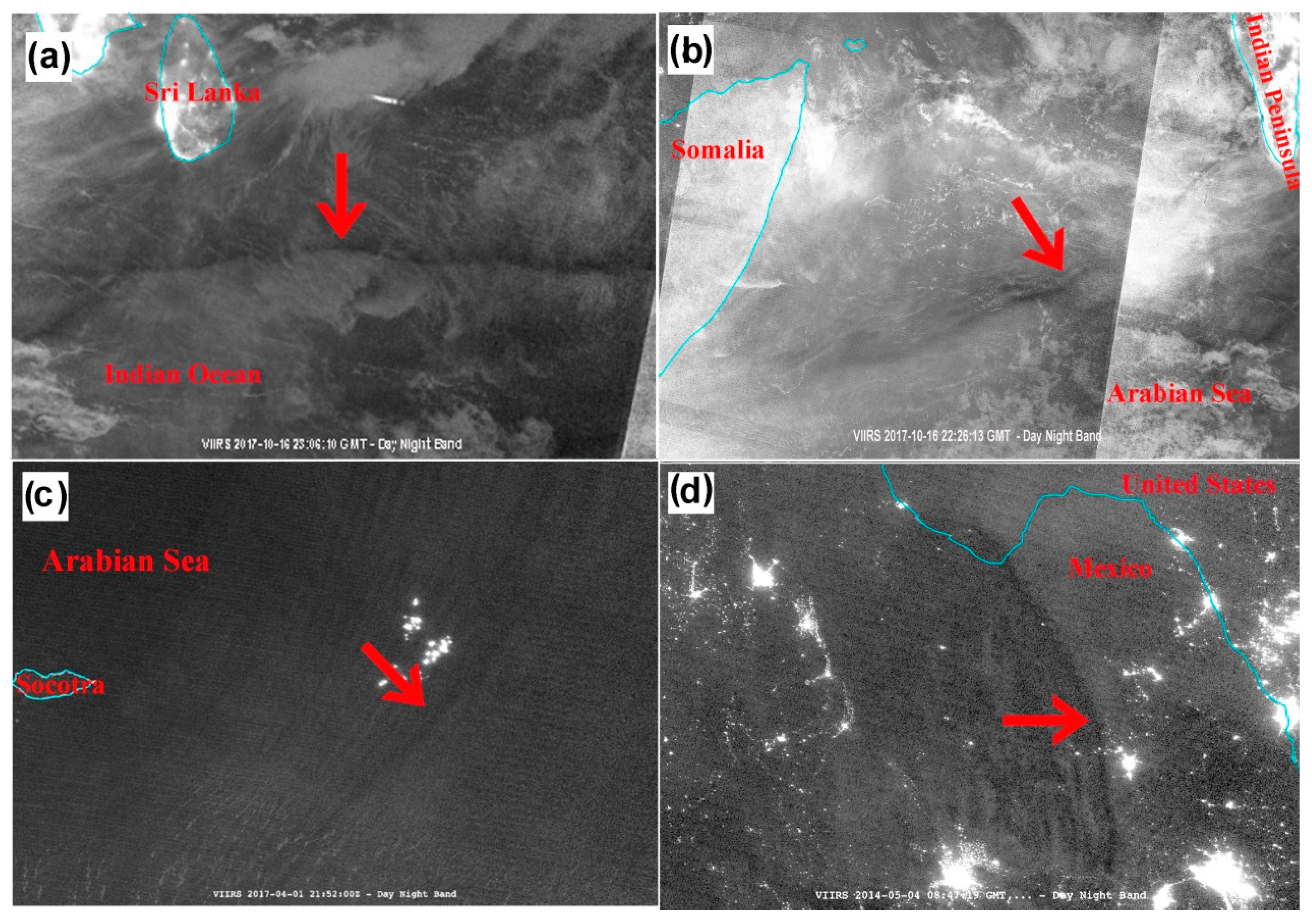
Figure 1 shows several examples of mesospheric bores detected in the DNB imagery during 2013–2017. Figure 1a shows a mesospheric bore observed over the north of the Indian Ocean at 23:06 UT on 16 October 2017. We can see that a clear horizontal line divided the nightglow sky into two parts, one darker to the north and the other brighter to the south. Small wave crests followed the frontal line. The mesospheric bore was wider than 2300 km (perpendicular to the propagation of the bore).
Figure 1b shows another extremely wide mesospheric bore observed over the Arabian Sea at 22:26 UT on 16 October 2017. It crossed the entire Arabian Sea, stretching from eastern Somalia to the southern Indian peninsula. Three small wave crests followed the bore front around the center of the bore. The width of the bore reached 3000 km.
Figure 1c shows a mesospheric bore observed over the Arabian Sea at 21:52 UT on 1 April 2017. The bore contained more than 15 trailing crests and troughs, extending 300 km behind the bore front. This is the largest number of trailing crests observed among the 61 bores considered in this study.
As a final example, a mesospheric bore near the Mexico and Texas border at 08:47 UT on 4 May 2014 is shown in Figure 1d. The bore extended from the south-east to the north-west. Like the other examples shown in Figure 1, this event was characterized by a typical darkening of the nightglow, followed by a sharp wave front and a series of trailing wave crests. The width of the mesospheric bore was about 1400 km and the average wavelength of the bore crests is estimated to be about 20 km.
Due to the limited temporal resolution of satellite observations, DNB cannot provide the bore evolution process. On the other hand, these extremely long mesospheric bores cannot be fully captured by a ground-based airglow imager. Thus, a ground-based airglow imager network has been developed in China [26].
3.2. A Mesospheric Bore Observed from both Space and the Ground
The 4 May 2014 bore event was also observed by a ground-based airglow imager at the Boston University field station, McDonald Observatory (MDO) [6]. The Boston University imager uses three bare charge-coupled device (CCD) wide-angle imaging bands (557.7 nm (O(1S)), 589.3 nm (Na), (P1(6) doublet of OH(4-0) band) at MDO, Fort Davis, Texas (30.67°N, 104.02°W). The OH filter transmits OH emissions from 695 nm to 950 nm. The filter consists of a step function that exhibits 0% transmission blue-ward of 695 nm with 50% at 695 nm. The quantum efficiency (QE) of the CCD chip determines the red-end cutoff at 950 nm.
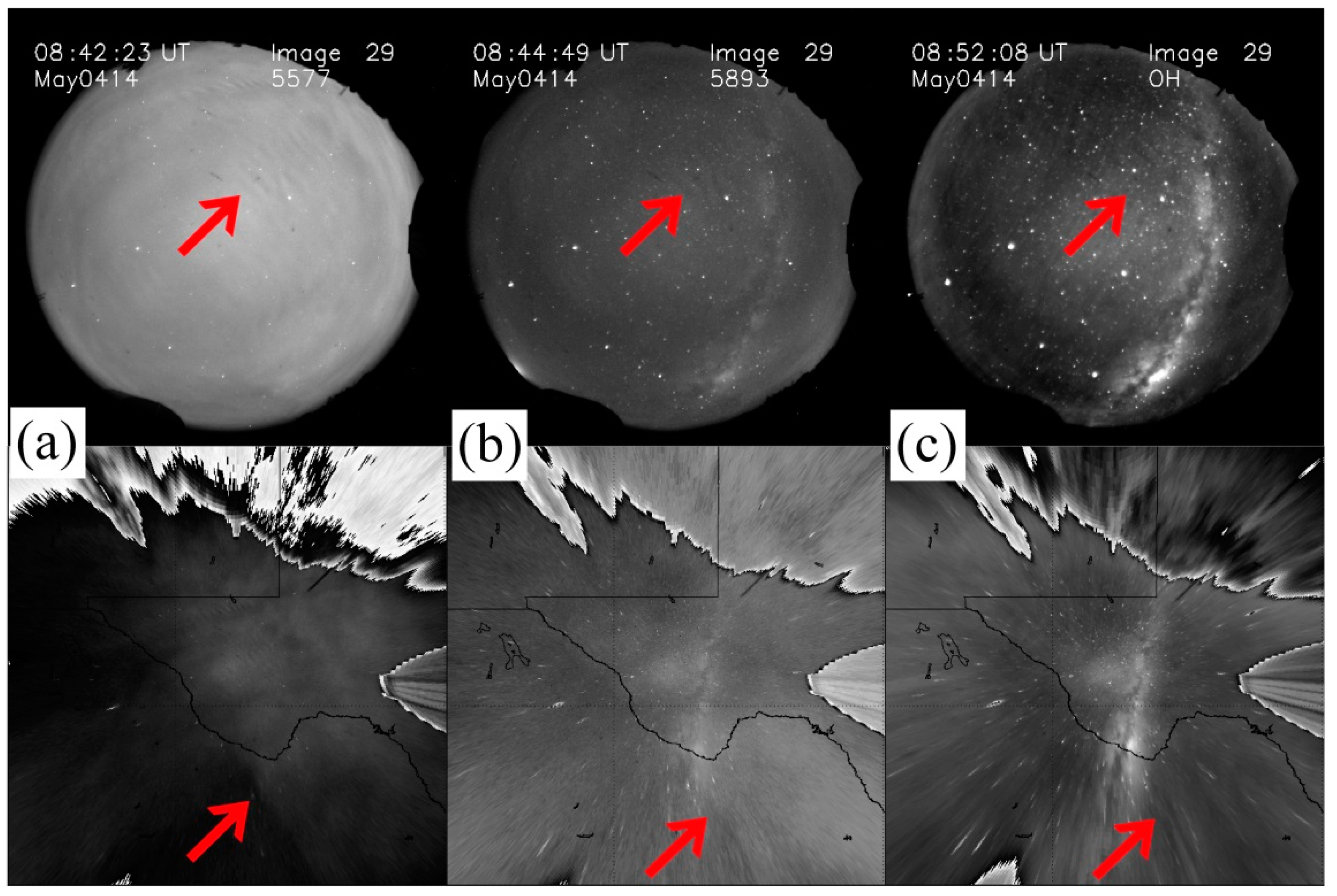
Figure 2 shows three raw all-sky images during the event from MDO in (a) 557.7 nm (O(1S)), (b) 589.3 nm (Na) and (c) 695~950 nm OH band emission (at the top) and corresponding unwrapped images (at the bottom) from 08:42 UT to 08:52 UT on 4 May 2014. The unwrapped image means that the image is geometrically corrected for lens distortion, and then mapped onto the Earth’s geographic coordinates for assumed airglow layer heights of 86 km (OH) [4], 90 km (Na) [27] and 96 km (O(1S)) [28]. The bore divided the sky into two parts of bright and dark halves in Figure 2a, and a series of crests and troughs followed.
When processing these ground-based airglow images, the nightglow background at a fixed location can be considered as a constant over a short period (e.g., 13 min used here) [23]. Hence, we subtracted two consecutive images to remove the background. These time-difference images can yield sharper bore fronts.
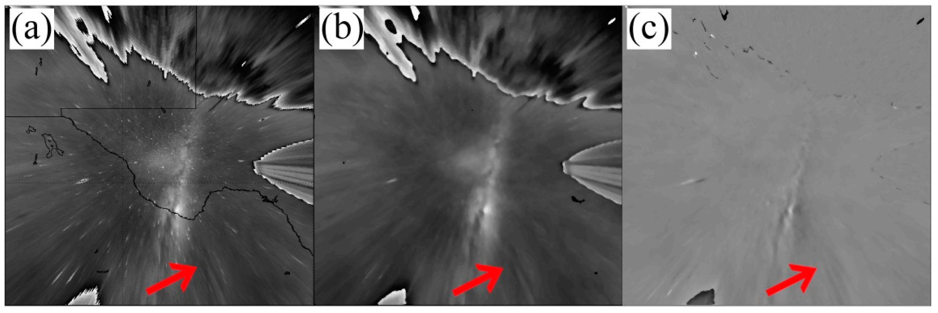
Figure 3 shows the unwrapped OH image (a), the 2D-median filtered image (b), and the time-difference image (c) of the mesospheric bore event at 08:52 UT on 4 May 2014. By using a 2D-median filter we largely removed the stars from the image (Figure 3b), and time-difference images eliminate the background as mentioned above. Across this 13-min sampling interval, stars moved slightly in the sky, thus becoming vertical lines in Figure 3c.
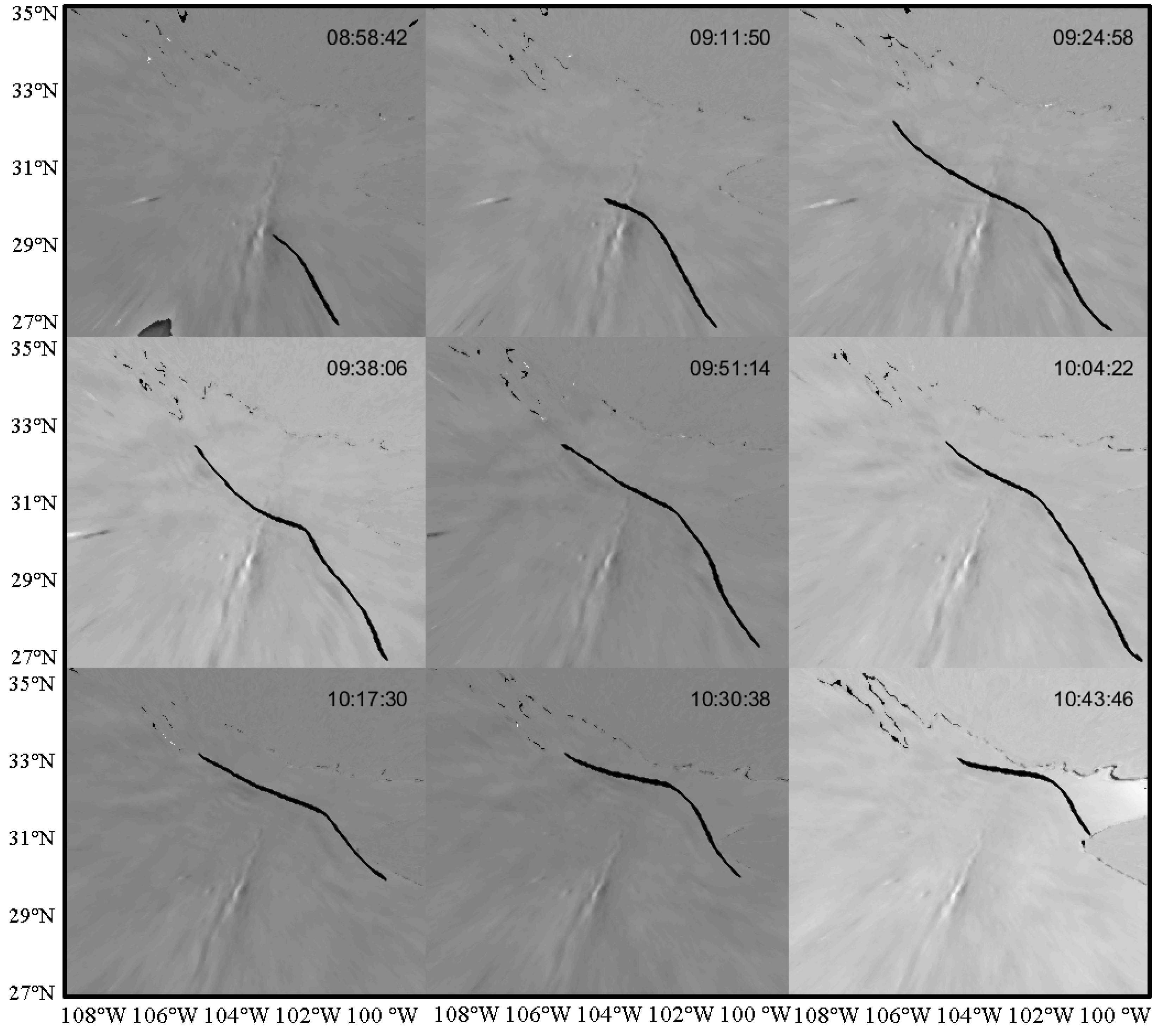
Figure 4 displays a time series of time-differenced OH images of the mesospheric bore event as seen by the airglow imager on 4 May 2014. The event continued for over four hours until dawn. The black line in the figure underscores the bore front, and each image is in the 900 × 900 km2 area. By following the bore front in time, we can determine the average horizontal speed of the bore to be 78 ± 5 m·s−1. Previous bore events have reported bore speeds between 50 m·s−1 and 100 m·s−1 [1,6,7,9,29].
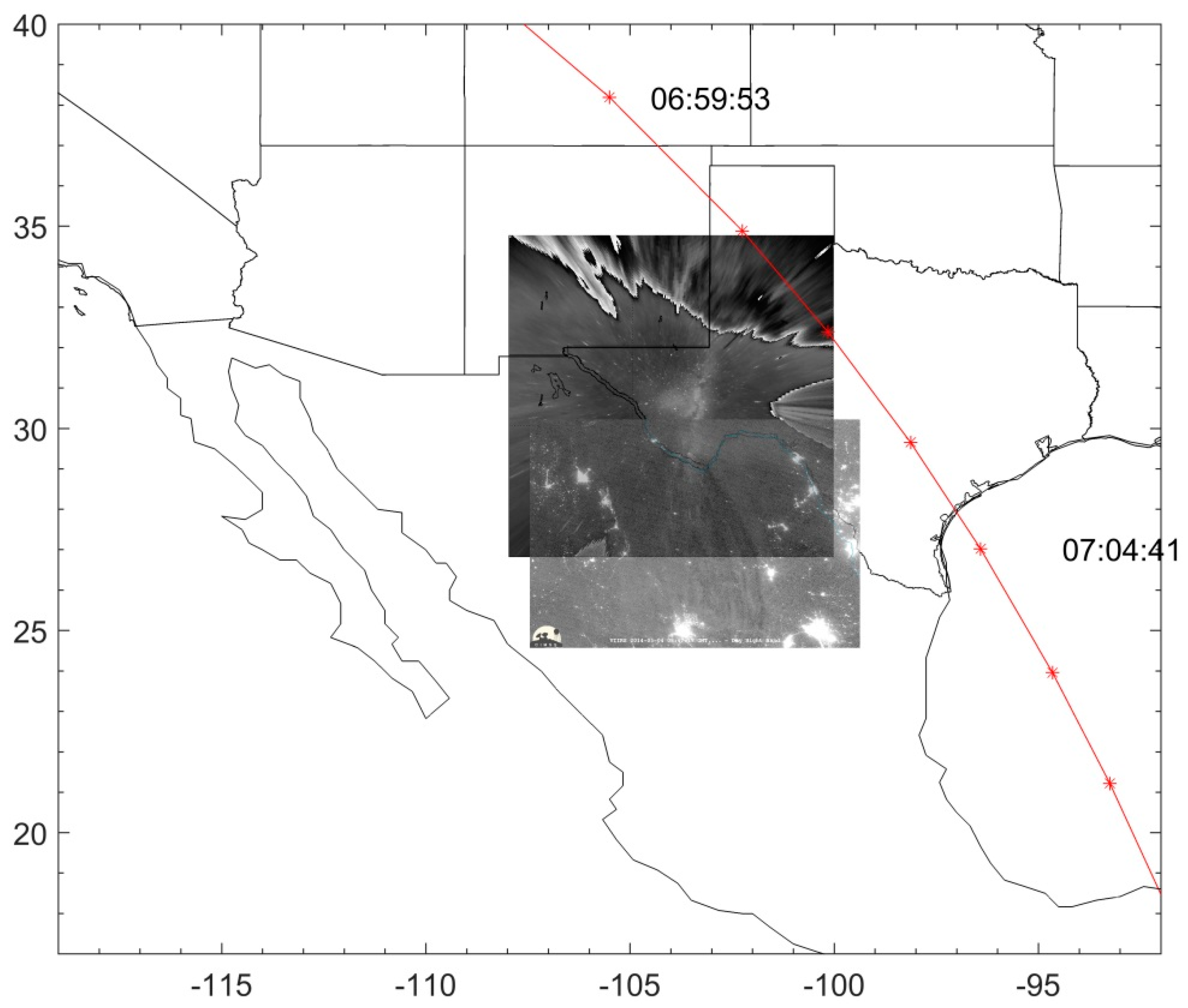
Bore propagation in the atmosphere is often supported by a temperature inversion layer [6,7,8,9]. Mesospheric bores, in particular, require a stable ducting layer supported by a temperature inversion or wind shear [1]. To examine this condition for the 4 May 2014 bore event, we analyzed the Sounding of the Atmosphere using Broadband Emission Radiometry (SABER) temperature data [30]. Two hours prior to the bore event, around 7 UT, the NASA Thermosphere, Ionosphere, Mesosphere, Energetics and Dynamics (TIMED) satellite passed over the MDO site and SABER obtained the OH emission and neutral temperature profiles. In Figure 5, the red line denotes the orbit of SABER on 4 May 2014.
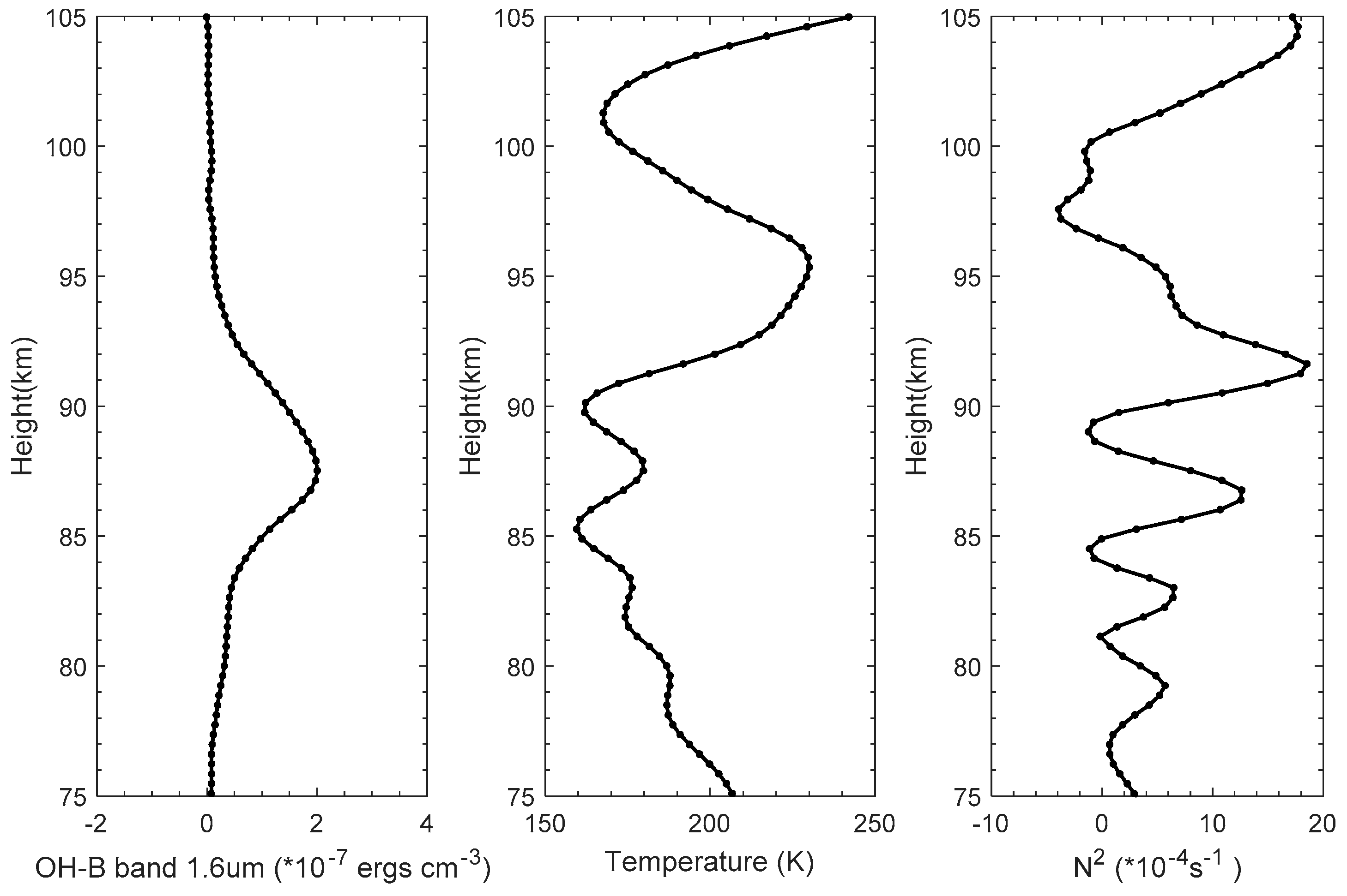
Figure 6 shows the averaged vertical profiles of OH emission and temperature obtained by SABER at 06:59 to 07:06 UT. The square of the Brunt–Vaisala frequency N2 is expressed as:
where g is 9.54 m·s−2, θ is the potential temperature at the bore altitude, and θ = T(P0/P)0.288. Maximum OH emission occurred at 87 km with a full width at half maximum (FWHM) thickness of 4 km (Figure 6a). The temperature profile exhibited a ~60 K temperature inversion between 90 km and 96 km (Figure 6b). This strong temperature inversion provided a ducting region centered near 93 km altitude with a FWHM width of 3.5 km (Figure 6c). Mesospheric temperature inversion layers are often long-lasting phenomena, so it is reasonable to assume that the temperature inversion still existed over Texas after two hours to support the mesospheric bore, maybe at lower altitudes.
Based on the hydraulic jump theory, Dewan and Picard [1] developed a simple model for the internal bore propagation in the mesosphere. In a shallow medium, the velocity (u0) and horizontal wavelength (λh) of an internal bore are dependent on the geometric thickness of the inversion layer (h0) via the following relationships:
where h0 and h1 represent the depth of the duct before and after the passage of the bore, respectively. The parameter g’ is the acceleration due to gravity corrected for buoyancy, such that g′ = g [(∆θ)/θ], where θ is the potential temperature at the bore altitude and θ = T (P0/P)0.288, ∆θ is the change in potential temperature from h0 to h1. g′ was calculated to be 1.04 m·s−2.
From the above equations, h0 was computed as ~3.5 km and u0 estimated to be 78 ± 5 m·s−1. The depth of the duct after the bore passage, h1, was calculated as ~4.9 km. Using these terms in Equation (3), the crest wavelength was found to be ~23 km. This is very close to the DNB observed value of 20 km. Previous bore events have reported that the wavelengths of the bore crests are between 15 km and 50 km [1,7,9,29].
The normalized bore strength β [31] can be written as:
when β < 0.3, the phase-locked waves behind the bore are stable, and this disturbance is called an undular bore. If β > 0.3, the bore may break and cause turbulence. Such bore is called a turbulent of foaming bore. In this bore event, the average β is 0.4, so we do not see a stable train of phase-locked waves behind the bore front most of the time in both the MDO imager and DNB image.
Ground-based bore observations have been performed by a number of studies for decades [5,6,7,8,9,14,17,20,21,29,32,33,34]. The ground-based imager analysis of this bore event confirms that DNB indeed observed the same mesospheric bore from space without temporal information. Moreover, on moonless nights, DNB provides a global view of mesospheric bores. Hence, a preliminary global morphology of mesospheric bore events is reported in the next section. We emphasize “preliminary” here because only clear bore events are identified from the dark background.
4. Discussion
Only DNB data under dark illumination conditions and a new moon is of value; that is, solar and lunar zenith angles must be greater than 108°. The offset corrected radiance data were remapped to a Mercator Projection, cropped to a maximum satellite zenith angle of 60° to avoid residual edge-of-scan noise patterns, scaled logarithmically between −11.5 to −9.0 W·cm−2·sr−1 [35]. So we only have about 420 ± 30 nights with airglow data during 2013–2017. The nightly viewing frequency from the satellite is 23 ± 2%. DNB observations were made for all seasons, but only data between 50°S and 50°N were included to exclude illumination from the aurora [35]. The mesospheric bores detected in DNB imagery over land surfaces (especially high-albedo surfaces such as snow and ice) may be more difficult. Additionally, city lights impair DNB’s imaging of mesospheric bores. A mask is used to exclude those areas with strong anthropogenic illumination [35]. Hence, only 61 mesospheric bore events observed by DNB during 2013–2017, 14.5 ± 2% from 420 ± 30 nights, are reported preliminarily. Some other bore events failed to be determined due to the unfavorable observation conditions. We identified the bore events as accurately as possible, but wall-type wave events [3,36,37,38] may be mixed. The features of the wall-type wave also seem to be similar to the mesospheric bore. The wall-type wave was caused by large-amplitude long-period upward-propagating gravity waves [4,36,38]. The characteristics of the change in airglow brightness, including the timescale, the phase relation of the changes between different emissions, and the airglow intensity depletion and cooling prior to the passage of the front, do not agree with the wall-type wave observation [4,36,38]. In particular, the timescale of the sharp increase of the airglow intensity is different: the wall-type wave took about 1 h to increase, whereas bore usually shows a timescale of minutes for the passage of the leading front [4,36,38]. In our study, the criterion we used to distinguish between bore events and wall wave events is the sharp wave front and the following shorter wavelength crests. Among the 61 events, 58 events were characterized by a sharp wave front and a series of trailing wave crests. The remaining three events had no obvious trailing wave crests in the nightglow, and therefore they can be either wall waves or turbulence bores. So, the ratio of confirmed bore events from all the bright events is about 95 ± 5%.
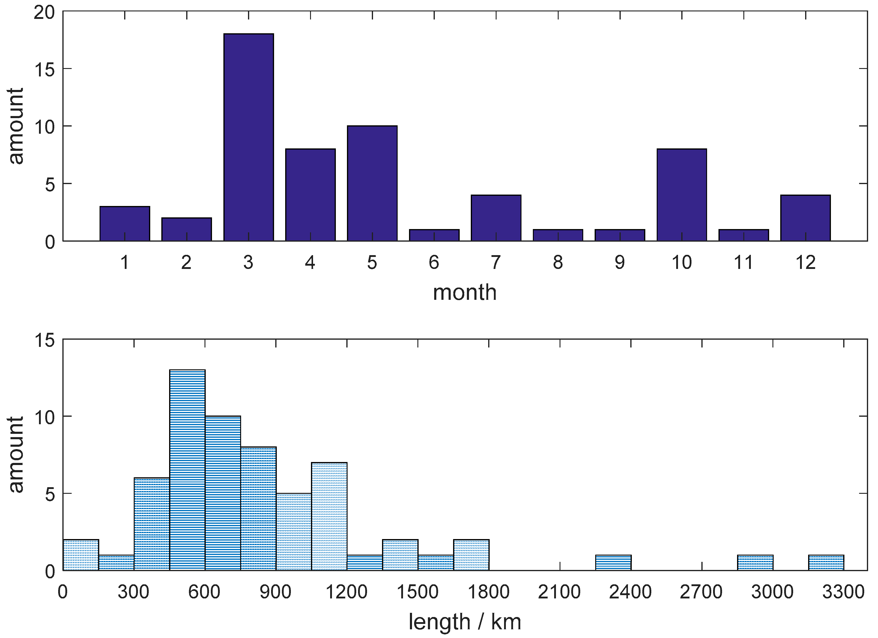
The months and lengths of 61 DNB mesospheric bore events from 2013 to 2017 are shown in Figure 7. Mesospheric bores occurred more frequently in March, April and May (36 events), accounting for 59% of the total bore events. Bores occurred eight times in October, accounting for 13% of the total events. Mesospheric bores propagation requires a stable ducting layer often being supported by a temperature inversion layer [1,6,7,8,9]. Non-linear interactions between gravity waves and tides [39] have been proposed as the origin of the inversion layer. In the mesosphere, the amplitude of the diurnal tide reaches its maximum during March/April. The diurnal tide is largest around equinoxes and is larger during the vernal equinox [40]. The mesospheric bore occurrence rate is the largest in March, April and May and is larger in October. This is consistent with the months of the diurnal tide peak amplitude in the mesosphere. Figure 7b (bottom) is the histogram showing the widths of the mesospheric bores. We can see that the widths of 49 mesospheric bores are between 300 and 1200 km, accounting for 80% of all bore events. The widest bore is ~3200 km. Ground-based observations have a limited field of view (e.g., MDO imager: 900 × 900 km). Therefore, it is common that ground-based observation can only observe a portion of the bore. Compared with a single airglow imager, the DNB observations can cover a wider spatial range and possibly observe the full extension of a mesospheric bore. This is a major advantage of satellite observations. In addition, cloudy conditions do not interfere with space observations.
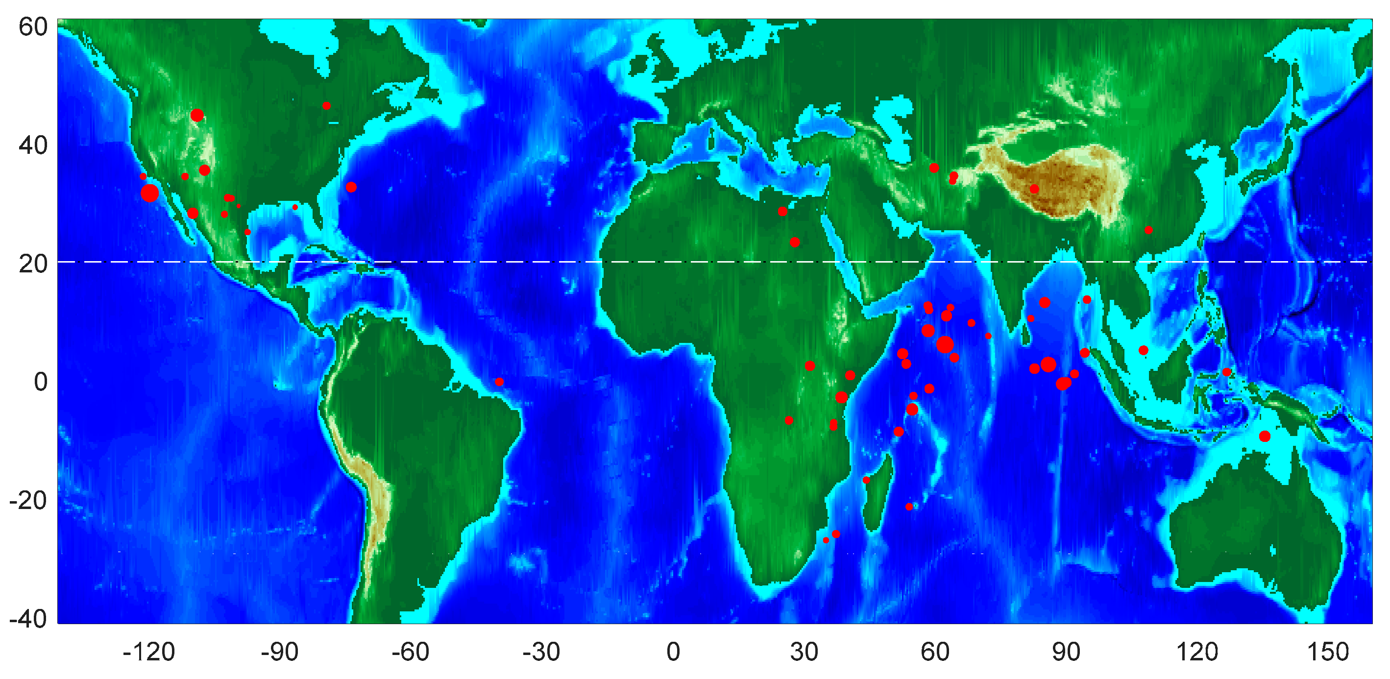
We also considered the geographic distribution of mesospheric bores, as shown in Figure 8. The contour in Figure 8 corresponds to the terrain height. The solid black dots indicate the locations where the bore events were seen, and the size of the dots is proportional to the width of the bore. Most of the mesospheric bore events occurred over the oceans or near the mountains, accounting for 72% of the total 61 bore events. They occurred 15 times and 8 times respectively over the Arabian Gulf of the Indian Ocean and the Gulf of Mexico. Moreover, they occurred 10 times near the Rocky Mountains in America, 7 times near the Kilimanjaro Mountains in Africa, and 4 times over the Asian Qinghai-Tibet Plateau. These findings may be an artifact of detectability over various backgrounds. As there are fewer background lights in the mountains and on the oceans, detectability of the faint nightglow structures is inherently better.
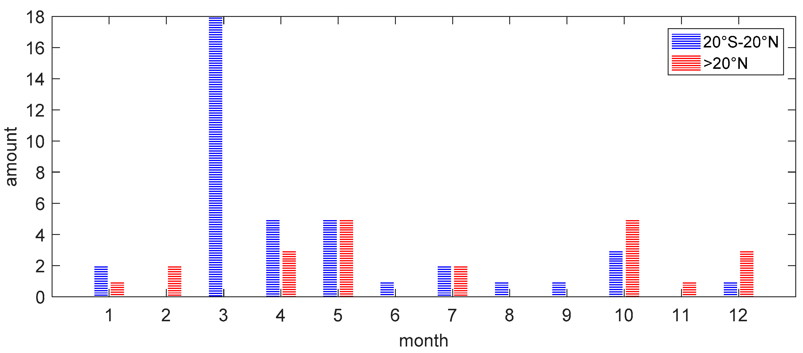
Taking the 20°N latitude as the dividing line, we counted the months in which bore events occurred at low latitudes and at middle latitudes, respectively (Figure 9). At middle latitudes (>20°N), bore events often took place in May and October. The bore events at low latitudes (20°S–20°N) mainly occurred in March and April, accounting for 57% of all bore events. The occurrence frequency of bore events at low latitudes is higher than that at middle latitudes. Among the 61 bore events, 39 events occurred at low latitudes. In the meantime, temperature inversion layers exhibit strong latitudinal and seasonal dependence. At low latitudes (20°S–20°N), the occurrence rate peaks in spring, with a maximum of 90%. The amplitude also reaches its maximum (40 K) in spring [41]. This is in good agreement with the occurrence rate of the DNB mesospheric bores: largest in March and April at low latitudes. Both the occurrence rate and amplitude of temperature inversion layers at middle latitudes are generally lower than at low latitudes [41]. The occurrence frequency of DNB bore events at middle latitude is lower than that at low latitudes.
5. Conclusions
In this paper, we report selected DNB imagery of mesospheric bores including wide mesospheric bore events extending 2000 km, and another mesospheric bore event with more than 15 trailing crests and troughs.
A mesospheric bore event over the Mexico/Texas border on 4 May 2014 was shown and analyzed together with ground-based airglow imager observations in more detail. This DNB bore observation is verified well. The entire bore front is wider than 1400 km and the propagation speed is about 78 ± 5 m·s−1. The average wavelength of the bore crests is about 20 km, which is consistent with previous bore studies [1,6,7,9,21,29]. A temperature inversion layer two hours before provided a ducting region centered near 93 km altitude with a FWHM of ~3.5 km. Based on the hydraulic jumping theory, the crest wavelength is calculated to be ~23 km, and it is very close to the DNB observed value of 20 km. The average bore strength β is 0.4, suggesting an unstable bore, and we see the unstable train of phase-locked waves behind the bore most of the time.
We also present some preliminary global morphology of DNB mesospheric bores from 2013 to 2017. (a) Most mesospheric events were characterized by a typical darkening of the nightglow and followed by a sharp wave front and a series of trailing wave crests. (b) Mesospheric bores occurred more frequently in March, April and May, which is consistent with the peak months of the diurnal tide in the mesosphere [39,40]. (c) More than 80% of these bores had widths between 300 and 1200 km. Three mesospheric bores were wider than 2000 km, and the widest mesospheric bore was found to be 3200 km. (d) The bore events at low latitudes mainly occurred in March and April. The bore occurrence frequency at low latitudes is higher than at middle latitudes. One of many possibilities is that both the occurrence rate and amplitude of temperature inversion layers at middle latitudes are generally lower than at low latitudes [41].
This paper demonstrates the unique capability of DNB observing mesospheric bores from space. While the horizontal propagation velocity and small wave crest addition rate can only be measured using ground airglow imagers, DNBs on two ongoing satellites (Suomi NPP and NOAA20) can observe mesospheric bores on a global scale. With both Suomi NPP and NOAA20 DNBs flying in the same orbit but ~50 min apart, it is feasible to derive the horizontal bore velocity from space. In order to understand the horizontal transport of energy and momentum via mesospheric bore propagations, a global survey of mesospheric bores using these two DNBs will be performed in a future study.
Author Contributions
Y.S., J.Y., and X.L. conceived the idea. Y.S., S.M., W.S., and S.S. provided and analyzed the data. Y.S. wrote the paper under the close guidance of J.Y., X.L., D.G., and S.G.
Funding
This research was funded by the National Science Foundation of China (91537213, 41875048) and National Natural Science Foundation Item (41675039).
Acknowledgments
Y.S. thanks Hampton University for hosting him during his visit. We thank the SABER/TIMED team for providing the temperature and the OH emission data (http://saber.gatsinc.com/index.php).
Conflicts of Interest
The authors declare no conflict of interest.
References
- Dewan, E.M.; Picard, R.H. Mesospheric bores. J. Geophys. Res. Atmos. 1998, 103, 6295–6305. [Google Scholar] [CrossRef] [Green Version]
- Dewan, E.M.; Picard, R.H. On the origin of mesospheric bores. J. Geophys. Res. 2001, 106, 2921–2927. [Google Scholar] [CrossRef] [Green Version]
- Swenson, G.R.; Espy, P.J. Observations of two-dimensional airglow structure and Na density from the ALOHA, 9 October 1993, “storm flight”. Geophys. Res. Lett. 1995, 22, 2845–2848. [Google Scholar] [CrossRef]
- Swenson, G.R.; Qian, J.; Plane, J.M.C.; Espy, P.J.; Taylor, J.J.; Turnbull, D.N.; Lowe, R.P. Dynamical and chemical aspects of the mesospheric Na “wall” event on 9 October 1993 during the ALOHA campaign. J. Geophys. Res. 1998, 103, 6361–6380. [Google Scholar] [CrossRef]
- Taylor, M.J.; Turnbull, D.N.; Lowe, R.P. Spectrometric and imaging measurements of a spectacular gravity wave event observed during the ALOHA-93 Campaign. Geophys. Res. Lett. 1995, 22, 2849–2852. [Google Scholar] [CrossRef] [Green Version]
- Smith, S.M.; Taylor, M.J.; Swenson, G.R.; She, C.Y.; Hocking, W.; Baumgardner, J.; Mendillo, M. A multidiagnostic investigation of the mesospheric bore phenomenon. J. Geophys. Res. Space Phys. 2003, 108, 1083. [Google Scholar] [CrossRef]
- Smith, S.M.; Friedman, J.; Raizada, S.; Tepley, C.; Baumgardner, J.; Mendillo, M. Evidence of mesospheric bore formation from a breaking gravity wave event: Simultaneous imaging and lidar measurements. J. Atmos. Sol. Terr. Phys. 2005, 67, 345–356. [Google Scholar] [CrossRef]
- She, C.Y.; Li, T.; Williams, B.P.; Yuan, T.; Picard, R.H. Concurrent OH imager and sodium temperature/wind lidar observation of a mesopause region undular bore event over Fort Collins/Platteville, Colorado. J. Geophys. Res. Atmos. 2004, 109, 107. [Google Scholar] [CrossRef]
- Yue, J.; She, C.Y.; Nakamura, T.; Harrell, S.; Yuan, T. Mesospheric bore formation from large-scale gravity wave perturbations observed by collocated all-sky OH imager and sodium lidar. J. Atmos. Sol. Terr. Phys. 2010, 72, 7–18. [Google Scholar] [CrossRef]
- Simkhada, D.B.; Snively, J.B.; Taylor, M.J.; Franke, S.J. Analysis and Modeling of Ducted and Evanescent Gravity Waves Observed in the Hawaiian Airglow. Ann. Geophys. 2009, 27, 3213–3224. [Google Scholar] [CrossRef]
- Laughman, B.; Fritts, D.C.; Werne, J. Numerical simulation of bore generation and morphology in thermal and Doppler ducts. Ann. Geophys. 2009, 27, 511–523. [Google Scholar] [CrossRef] [Green Version]
- Seyler, C.E. Internal waves and undular bores in mesospheric inversion layers. J. Geophys. Res. 2005, 110, D09S05. [Google Scholar] [CrossRef]
- Medeiros, A.F.; Taylor, M.J.; Takahashi, H.; Batista, P.P.; Gobbi, D. An unusual airglow wave event observed at Cachoeira Paulista 231S. Adv. Space Res. 2001, 27, 1749–1754. [Google Scholar] [CrossRef]
- Smith, S.M. The identification of mesospheric frontal gravity-wave events at a mid-latitude site. Adv. Space Res. 2013, 54, 417–424. [Google Scholar] [CrossRef]
- Brown, L.B.; Gerrard, A.J.; Meriwether, J.W.; Mekela, J.J. All-sky imaging of mesospheric fronts in OI 557.7 nm and broadband OH airglow emissions: Analysis of frontal structure, atmospheric background conditions and potential sourcing mechanisms. J. Geophys. Res. 2004, 109, D19104. [Google Scholar] [CrossRef]
- Fechine, J.; Medeiros, A.F.; Buriti, R.A.; Takahashi, H.; Gobbi, D. Mesospheric bore events in the equatorial middle atmosphere. J. Atmos. Sol. Terr. Phys. 2005, 67, 1774–1778. [Google Scholar] [CrossRef]
- Shiokawa, K.; Suzuki, S.; Otsuka, Y.; Ogawa, T.; Nakamura, T.; Mlynczak, M.; Russell, J.M. A multi-instrument measurement of a mesospheric front-like structure at the equator. J. Meteorol. Soc. Jpn. 2006, 84A, 305–316. [Google Scholar] [CrossRef]
- Li, Q.; Xu, J.; Yue, J.; Liu, X.; Yuan, W.; Ning, B.; Guan, S.; Younger, J.P. Investigation of a mesospheric bore event over northern China. Ann. Geophys. 2013, 31, 409–418. [Google Scholar] [CrossRef] [Green Version]
- Miller, S.D.; Straka, W.C., III; Yue, J.; Smith, S.M.; Alexander, M.J.; Hoffmann, L.; Setvák, M.; Partain, P.T. Upper atmospheric gravity wave details revealed in nightglow satellite imagery. Proc. Natl. Acad. Sci. USA 2015, 112, E6728–E6735. [Google Scholar] [CrossRef]
- Medeiros, A.F.; Paulino, I.; Taylor, M.J.; Fechine, J.; Takahashi, H.; Buriti, R.A.; Wrasse, C.M. Twin mesospheric bores observed over Brazilian equatorial region. Ann. Geophys. 2016, 34, 91–96. [Google Scholar] [CrossRef]
- Smith, S.M.; Stober, G.; Jacobi, C.; Chau, J.L.; Gerding, M.; Mlynczak, M.G.; Umbriaco, G. Characterization of a double mesospheric bore over Europe. J. Geophys. Res. Space Phys. 2017, 122, 9738–9750. [Google Scholar] [CrossRef]
- Miller, S.D.; William, S.; Stephen, P.M.; Christopher, D.E.; Thomas, F.L.; Jeremy, S.; Andi, W.; Andrew, K.H.; Stephanie, C.W. Illuminating the capabilities of the Suomi NPP VIIRS Day/Night Band. Remote Sens. 2013, 5, 6717–6766. [Google Scholar] [CrossRef]
- Schueler, C.F.; Lee, T.F.; Miller, S.D. VIIRS constant spatial-resolution advantages. Int. J. Rem. Sens. 2013, 34, 5761–5777. [Google Scholar] [CrossRef]
- Mills, S.P.; Miller, S.D. VIIRS Day/Night Band—Correcting striping and nonuniformity over a very large dynamic range. J. Imaging 2016, 2, 9. [Google Scholar] [CrossRef]
- Miller, S.D.; Combs, C.; Kidder, S.Q.; Lee, T.F. Assessing global and seasonal lunar availability for nighttime low-light visible remote sensing applications. J. Ocean. Atmos. Tech. 2012, 29, 538–557. [Google Scholar] [CrossRef]
- Xu, J.; Li, Q.; Yue, J.; Hoffmann, L.; Straka, W.C., III; Wang, C.; Liu, M.; Yuan, W.; Han, S.; Miller, S.D.; et al. Concentric gravity waves over northern China observed by an airglow imager network and satellites. J. Geophys. Res. Atmos. 2015, 120, 11–58. [Google Scholar] [CrossRef]
- Newman, A.L.; Nighttime, N.D. Emission observed from a polar-orbiting DMSP satellite. J. Geophys. Res. 1988, 93, 4067–4075. [Google Scholar] [CrossRef]
- Donahue, T.M.; Guenther, B.; Thomas, R.J. Distribution of atomic oxygen in the upper atmosphere deduced from Ogo 6 airglow observations. J. Geophys. Res. 1973, 78, 6662–6689. [Google Scholar] [CrossRef]
- Stockwell, R.G.; Taylor, M.J.; Nielsen, K.; Jarvis, M.J. The evolution of a breaking mesospheric borewave packet. J. Geophys. Res. 2011, 116, D19102. [Google Scholar] [CrossRef]
- Russell, J.M., III; Mlynczak, M.G.; Gordley, L.L.; Tansock, J.; Esplin, R. An overview of the SABER experiment and preliminary calibration results. Proc. SPIE 1999, 3756, 277–288. [Google Scholar]
- Lighthill, M.J. Waves in Fluids; Cambridge University Press: New York, NY, USA, 1978; p. 504. [Google Scholar]
- Neilson, K.; Taylor, M.J.; Stockwell, R.G.; Jarvis, M.J. An unusual mesospheric bore event observed at high latitudes over Antarctica. Geophys. Res. Lett. 2006, 33, L07803. [Google Scholar]
- Narayanan, V.L.; Gurubaran, S.; Emperumal, K. A case study of a mesospheric bore event observed with an all sky airglow imager at Tirunelveli (8.7°N). J. Geophys. Res 2009, 114, D08114. [Google Scholar] [CrossRef]
- Narayanan, V.L.; Gurubaran, S.; Emperumal, K. Nightglow imaging of different types of events, including a mesospheric bore observed on the night of 15 February 2007 from Tirunelveli (8.7°N). J. Atmos. Sol. Terr. Phys. 2012, 78–79, 70–83. [Google Scholar] [CrossRef]
- Miller, S.D.; William, S.P.; Elvidge, C.D.; Lindsy, D.T.; Lee, T.F.; Hawkins, J.D. Suomi satellite brings to light a unique frontier of nighttime environmental sensing capabilities. Proc. Natl. Acad. Sci. 2012, 109, 15706–15711. [Google Scholar] [CrossRef] [PubMed] [Green Version]
- Bageston, J.V.; Wrasse, C.M.; Hibbins, R.E.; Batista, P.P.; Gobbi, D.; Takahashi, H.; Fritts, D.C.; Andrioli, V.F.; Fechine, J.; Denardini, C.M. Case study of a mesospheric wall event over Ferraz station, Antarctica (62°S). Ann. Geophys. 2011, 29, 209–219. [Google Scholar] [CrossRef]
- Batista, P.P.; Clemesha, B.R.; Simonich, D.M.; Taylor, M.J.; Takahashi, H.; Gobbi, D.; Batista, I.S.; Buriti, R.A.; Medeiros, A.F. Simultaneous lidar observation of a sporadic sodium layer, a “wall” event in the OH and OI 5577 airglow images and the meteor winds. J. Atmos. Sol. Terr. Phys. 2002, 64, 1327–1335. [Google Scholar] [CrossRef]
- Li, F.; Swenson, G.R.; Liu, A.; Taylor, M.; Zhao, Y. Investigation of a “wall” wave event. J. Geophys. Res. 2007, 112, D04104. [Google Scholar] [CrossRef]
- Liu, H.; Hagan, M.E. Local heating/cooling of the mesosphere due to gravity wave and tidal coupling. Geophys. Res. Lett. 1998, 25, 2941–2944. [Google Scholar] [CrossRef] [Green Version]
- Xu, J.; Smith, A.K.; Liu, H.L.; Yuan, W.; Wu, Q.; Jiang, G.; Mlynczak, M.G.; Russell, J.M., III; Franke, S.J. Seasonal and quasi-biennial variations in the migrating diurnal tide observed by Thermosphere, Ionosphere, Mesosphere, Energetics and Dynamics (TIMED). J. Geophys. Res. 2009, 114, D13107. [Google Scholar] [CrossRef]
- Gan, Q.; Zhang, S.D.; Yi, F. TIMED/SABER observations of lower mesospheric inversion layers at low and middle latitudes. J. Geophys. Res. 2012, 117, D07109. [Google Scholar] [CrossRef]
Figure 1.
Mesospheric bore events observed by Suomi National Polar-orbiting Partnership Visible/Infrared Imaging Radiometer Suite Day/Night Band (Suomi-NPP VIIRS DNB) over: (a) Indian Ocean, at 23:06 UT on 16 October 2017; (b) Arabian Sea, at 22:26 UT on 16 October 2017; (c) Arabian Sea, at 21:52 UT on 4 April 2017; (d) Mexico, at 8:47 UT on 4 May 2014. The red arrows indicate the mesospheric bore fronts and their propagation directions.

Figure 2.
Three raw all-sky images from the McDonald Observatory (MDO) in (a) 557.7 nm (O(1S)), (b) 589.3 nm (Na) and (c) 695~950 nm (P1(6) doublet of OH(4-0) band) emission at ~08:45 on 4 May 2014 (top), and three corresponding unwrapped images (bottom).
Figure 2.
Three raw all-sky images from the McDonald Observatory (MDO) in (a) 557.7 nm (O(1S)), (b) 589.3 nm (Na) and (c) 695~950 nm (P1(6) doublet of OH(4-0) band) emission at ~08:45 on 4 May 2014 (top), and three corresponding unwrapped images (bottom).

Figure 3.
(a) Unwrapped OH image of the mesospheric bore event at 08:52 UT 4 May 2014, (b) 2D-median filtered image, (c) time-difference image.
Figure 3.
(a) Unwrapped OH image of the mesospheric bore event at 08:52 UT 4 May 2014, (b) 2D-median filtered image, (c) time-difference image.

Figure 4.
Time-difference OH images of the mesospheric bore event on 4 May 2014. The observation UT time is given at the top of each image. The black line indicates the front of the mesospheric bore.
Figure 4.
Time-difference OH images of the mesospheric bore event on 4 May 2014. The observation UT time is given at the top of each image. The black line indicates the front of the mesospheric bore.

Figure 5.
TIMED/SABER instrument descending footprints in the field of view during the bore event on 4 May 2014.
Figure 5.
TIMED/SABER instrument descending footprints in the field of view during the bore event on 4 May 2014.

Figure 6.
Averaged vertical profiles of OH emission, temperature and square of the Brunt–Vaisala frequency (N2) obtained by Sounding of the Atmosphere using Broadband Emission Radiometry (SABER) measurements from 06:59 to 07:06 UT, 2 h prior to mesospheric bore onset on 4 May 2014.
Figure 6.
Averaged vertical profiles of OH emission, temperature and square of the Brunt–Vaisala frequency (N2) obtained by Sounding of the Atmosphere using Broadband Emission Radiometry (SABER) measurements from 06:59 to 07:06 UT, 2 h prior to mesospheric bore onset on 4 May 2014.

Figure 7.
Mesospheric bore occurrence months (top) and the bore widths based on the 61 events (bottom).
Figure 7.
Mesospheric bore occurrence months (top) and the bore widths based on the 61 events (bottom).

Figure 8.
Locations of 61 mesospheric bores. Map colors indicate the terrain height, with the blue representing the oceans. The solid red dots indicate the locations where the mesospheric bore events were detected by the DNB, and the size of the dots denotes the widths of the bores.
Figure 8.
Locations of 61 mesospheric bores. Map colors indicate the terrain height, with the blue representing the oceans. The solid red dots indicate the locations where the mesospheric bore events were detected by the DNB, and the size of the dots denotes the widths of the bores.

Figure 9.
Mesospheric bore months at different latitudes. Blue denotes the tropical region (20°S–20°N); red denotes the region north of 20°N.
Figure 9.
Mesospheric bore months at different latitudes. Blue denotes the tropical region (20°S–20°N); red denotes the region north of 20°N.

© 2018 by the authors. Licensee MDPI, Basel, Switzerland. This article is an open access article distributed under the terms and conditions of the Creative Commons Attribution (CC BY) license (http://creativecommons.org/licenses/by/4.0/).
Share and Cite
MDPI and ACS Style
Su, Y.; Yue, J.; Liu, X.; Miller, S.D.; Straka, W.C., III; Smith, S.M.; Guo, D.; Guo, S. Mesospheric Bore Observations Using Suomi-NPP VIIRS DNB during 2013–2017. Remote Sens. 2018, 10, 1935. https://doi.org/10.3390/rs10121935
AMA Style
Su Y, Yue J, Liu X, Miller SD, Straka WC III, Smith SM, Guo D, Guo S. Mesospheric Bore Observations Using Suomi-NPP VIIRS DNB during 2013–2017. Remote Sensing. 2018; 10(12):1935. https://doi.org/10.3390/rs10121935
Chicago/Turabian StyleSu, Yucheng, Jia Yue, Xiao Liu, Steven D. Miller, William C. Straka, III, Steven M. Smith, Dong Guo, and Shengli Guo. 2018. "Mesospheric Bore Observations Using Suomi-NPP VIIRS DNB during 2013–2017" Remote Sensing 10, no. 12: 1935. https://doi.org/10.3390/rs10121935
Note that from the first issue of 2016, this journal uses article numbers instead of page numbers. See further details here.