Article

Modeling Spatiotemporal Population Changes by Integrating DMSP-OLS and NPP-VIIRS Nighttime Light Data in Chongqing, China

1
School of Geographical Sciences, Southwest University, Chongqing 400715, China
2
The State Cultivation Base of Eco-Agriculture for Southwest Mountainous Land, Southwest University, Chongqing 400715, China
3
Institute of Green Low-Carbon Development, Southwest University, Chongqing 400715, China
*
Author to whom correspondence should be addressed.
The authors contributed equally to this work.
Remote Sens. 2021, 13(2), 284; https://doi.org/10.3390/rs13020284
Submission received: 10 December 2020 / Revised: 10 January 2021 / Accepted: 12 January 2021 / Published: 15 January 2021
(This article belongs to the Special Issue Nighttime Lights as a Proxy for Economic Performance of Regions)

Abstract

:
The sustained growth of non-farm wages has led to large-scale migration of rural population to cities in China, especially in mountainous areas. It is of great significance to study the spatial and temporal pattern of population migration mentioned above for guiding population spatial optimization and the effective supply of public services in the mountainous areas. Here, we determined the spatiotemporal evolution of population in the Chongqing municipality of China from 2000–2018 by employing multi-period spatial distribution data, including nighttime light (NTL) data from the Defense Meteorological Satellite Program’s Operational Linescan System (DMSP-OLS) and the Suomi National Polar-orbiting Partnership Visible Infrared Imaging Radiometer Suite (NPP-VIIRS). There was a power function relationship between the two datasets at the pixel scale, with a mean relative error of NTL integration of 8.19%, 4.78% less than achieved by a previous study at the provincial scale. The spatial simulations of population distribution achieved a mean relative error of 26.98%, improved the simulation accuracy for mountainous population by nearly 20% and confirmed the feasibility of this method in Chongqing. During the study period, the spatial distribution of Chongqing’s population has increased in the west and decreased in the east, while also increased in low-altitude areas and decreased in medium-high altitude areas. Population agglomeration was common in all of districts and counties and the population density of central urban areas and its surrounding areas significantly increased, while that of non-urban areas such as northeast Chongqing significantly decreased.

Graphical Abstract

1. Introduction

Urban-rural migration is a major issue affecting the sustainable development of society, while the spatial distribution of population is a core focus of research in population geography [1]. Driven by economic globalization, developing countries occupy an increasing share of the world economy and the world’s economic center continues to move to Asia [2,3,4]. As the largest developing country, China has experienced an unprecedented growth rate over the past 30 years. The urbanization rate has increased from 26% to 58% and the growth rate is about 2.7 times the world average (World Bank). China’s rapidly developing social economy and ongoing urbanization has resulted in the relocation and reorganization of urban and rural populations [5,6,7,8] as reflected in the continuous growth of the former and substantial reductions in the latter’s labor force. According to the National Bureau of Statistics of China (NBSC), the country’s urban population has increased by an average of 21 million per year since 2000. In contrast, the agricultural labor force has decreased by 11 million per year [9] and the rural population has decreased by ~30.2%, from 808 million in 2000 to 564 million in 2018 (NBSC). It is worth noting that population migration from mountainous areas has been particularly significant [9]. The process of urban-rural migration results in the redistribution of production factors such as capital, which will impact on the ecosystem and social economy, with contradiction between resources, the environment and population changing accordingly [10,11,12]. The rural population structure has also changed (including age, gender and number), which has changed the land use pattern and human activities radius, thereby affecting the construction and restoration of rural ecological civilization [6,13,14,15]. Therefore, mapping and estimating the spatial distribution of populations can provide scientific support for developing regionally sustainable development strategies and spatial land-use planning [16,17].
Traditional demographic statistics and analysis mainly rely on population surveys, including censuses and sampling studies. Until now, China has carried out six censuses. Although population surveys are scientific and authoritative [10,18], their data acquisition cycle is long and townships are the smallest survey unit, such that the spatial resolution of the data is insufficient [19]. Therefore most studies do not use the administrative unit as the research object [13,20,21]. With the rapid development of geographic information system and remote sensing technology, multi-source remote sensing data have been widely applied in spatial population research, especially land-use and night-time light (NTL) data [19,22,23,24,25,26,27,28,29]. For example, Yang et al. [24] combined Defense Meteorological Satellite Program’s Operational Linescan System (DMSP-OLS) NTL data, enhanced vegetation index data and digital elevation model (DEM) data to simulate the population density of Zhejiang. Hu et al. [25] determined the spatial distribution of population in Sichuan and Chongqing based on NTL data and land-use data. Other studies have shown that the spatial distribution of regional populations can be well-described by data processing, multi-source data fusion and model improvement [24,30]. Most research has remained focused on the spatial modeling of population at a single point in time [19,23,29,31,32], however few studies adopt multivariate data to model the population spatial distribution in a long time series.
Although the DMSP-OLS dataset provides continuous NTL data from 1992 to 2013 [33], its imagery contains problems due to OLS limitations such as discontinuity and oversaturation by bright lights [34,35] These data were replaced by Suomi National Polar-orbiting Partnership Visible Infrared Imaging Radiometer Suite (NPP-VIIRS) NTL data after 2013, bringing clear upgrades such as improved spatial resolution and reduced saturation [33] as well as on-board calibration [36]. Although these are clear upgrades, they also present challenges to obtaining consistent long-term NTL data [35,37,38], such that proper integration of the two datasets must be accomplished before the construction of a long-term population spatial distribution dataset and there have been several attempts to integrate DMSP and VIIRS NTL data [37,38,39,40,41]. Zhu et al. [39] established the relationship between the two at the provincial level and used it to model China’s Gross Domestic Product. Zhao et al. [37] achieved this at the pixel level and established a long-term NTL dataset in Southeast Asia. Previous studies have contributed to enhancing the consistency of NTL between DMSP and VIIRS data, however there are limitations regarding a widespread application of current methods, such as the models proposed has regional limitations and may not be suitable for other regions [37,41]; the datasets used are not accessible to general public [40,41]; and the time series of data generated only has consistent NTL indices at the administrative level and is still limited at the pixel level [39].
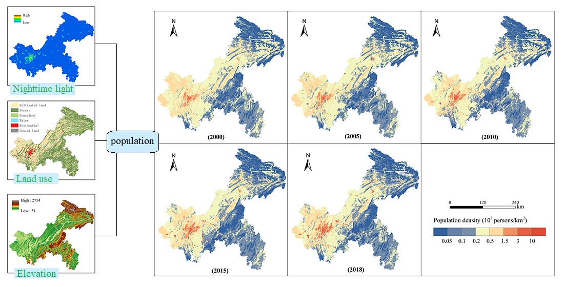
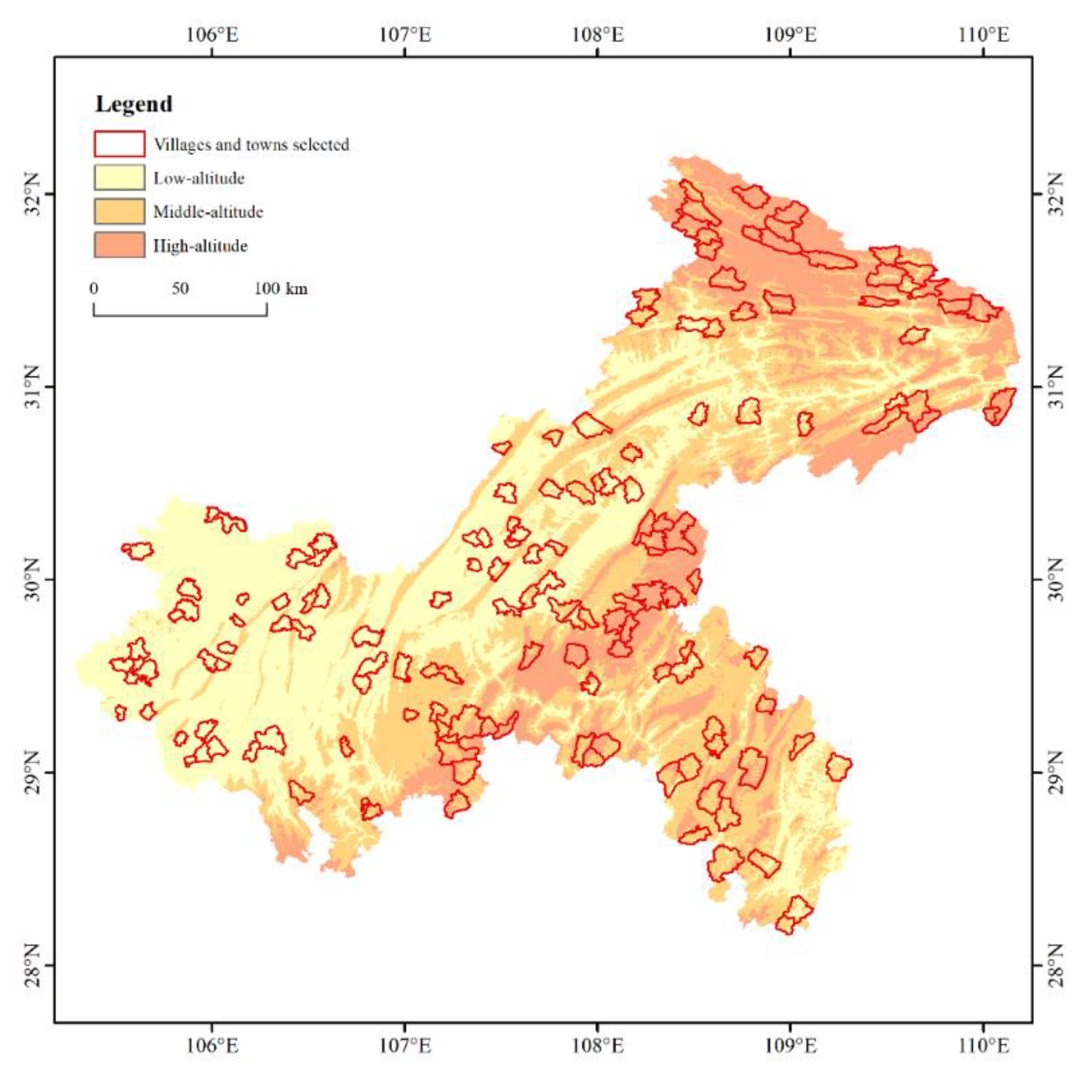
The municipality of Chongqing integrates a metropolis and a large rural area that is mostly mountainous area, which is characterized by intense human activities and a fragile ecological environment. According to the NBSC, ongoing urbanization in Chongqing resulted in the rural population declining from 15.33 million to 10.7 million from 2005 to 2018 (a decrease of 30.2%), exceeding the national average of 24.34%. Meanwhile, Chinese policies targeting poverty alleviation and rural revitalization have benefitted most residents in poor mountainous areas through relocation, resulting in major changes in population distribution. Therefore, exploring the spatiotemporal changes in Chongqing’s population via a timely understanding of population distribution data can help guide population migration from mountainous areas, promote the sustainable development of the regional economy and inform ecological restoration in mountainous areas.
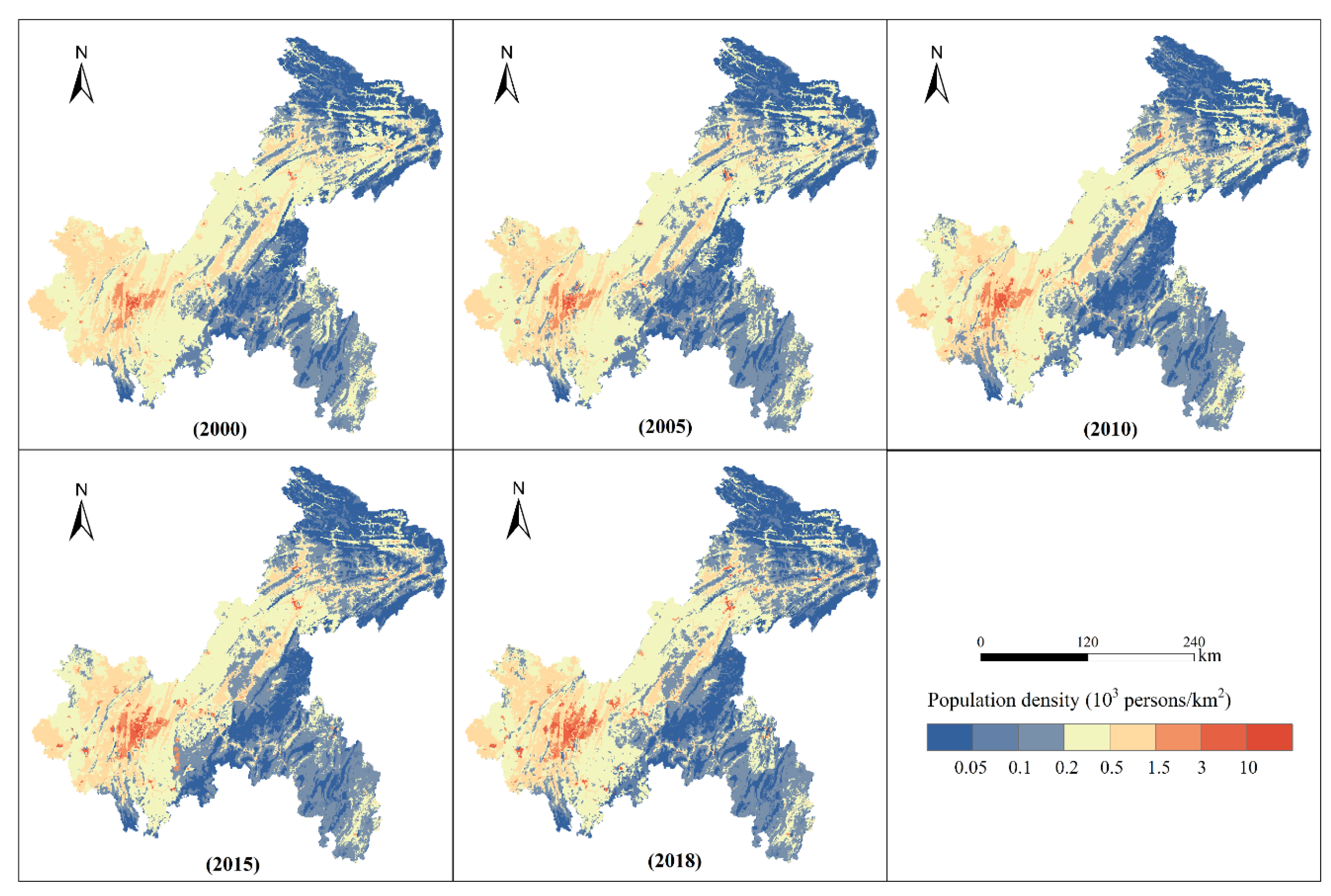
This study explored integration methods for the two NTL datasets that are suitable for the study area at the pixel level and constructed a long-term NTL dataset that provides a basis for modeling long-term population spatial distribution data. Then it simulated the spatial distribution of Chongqing’s population in 2000, 2005, 2010, 2015 and 2018 by integrating the two NTL datasets and analyzing spatiotemporal changes. Our results can serve as a scientific reference for rationally allocating urban and rural resources, optimizing urban and rural spatial patterns and promoting the high-quality development of the regional economy.

2. Study Area and Data

2.1. Study Area

Chongqing is located in the eastern Sichuan Basin, covering 8.24 × 10⁴ km2 from 28°10′–32°13′ N and 105°11′–110°11′ E (Figure 1). Its 26 districts and 12 counties cover a rugged landscape that is 75.33% mountainous. Its location at the intersection of the Silk Road and the Yangtze River Economic Belt allows it to form connections between east and west while driving economic development between north and south, leading to a vital role in China’s development strategy underlain by the Belt and Road Initiatives and Yangtze River Economic Belt [42]. Chongqing is one of the important population areas in Western China, having a resident population of 31.02 million in 2018, an increase of 2.53 million compared with 2000 (NBSC); its average population density is about three times the national average. Its location in the upper reaches of the Yangtze River is part of an ecological protective screen within the Yangtze River Economic Belt. Its complex topography and fragile ecological environment enhance tensions between humans and the environment, such that ecological construction and regional development face many challenges.

2.2. Data Sources

DMSP-OLS Version 4 NTL data from 2000 to 2013 were obtained from the Paynes Institute for Public Policy, Colorado School of Mines (https://eogdata.mines.edu/dmsp/downloadV4composites.html). These have a spatial resolution of 30 arc-seconds, with data values ranging from to 0–63 and have been denoised [43]. Monthly VIIRS Cloud Mask (vcm) data from 2013 to 2018 were also obtained from the Paynes Institute for Public Policy, Colorado School of Mines (https://eogdata.mines.edu/dmsp/download_radcal.html), with a spatial resolution of 15 arc-seconds that excludes observations affected by stray light. The data contained additional noise from sources such as auroras, fires, boats, other temporary lights and outliers, probably caused by stable lights from oil or gas fires.
Land-use data (1 km × 1 km) were obtained from the Resource and Environment Science Data Centre of the Chinese Academy of Sciences (http://www.resdc.cn/) with major categories including cultivated land, forest, grassland, water, residential land and unused land. Resident population data at the county level were obtained from the Chongqing Statistical Information Net (http://data.tjj.cq.gov.cn/), while those at the township level in 2015 were derived from the China County Statistical Yearbook 2016. DEM data were obtained from the Geospatial Data Cloud (http://www.gscloud.cn/).

2.3. Data Preprocessing

Firstly, all data were extracted by administrative boundaries and the DMSP-OLS NTL data was resampled to 1 km grids. Secondly, a stepwise calibration approach at the global scale was used to improve the temporal inconsistency of DMSP time series [44]. Thirdly, calculated the average value of VIIRS data from January to December to generate annual time series of VIIRS NTL imagery. Fourthly, mask extraction was then used to remove noise from the NPP-VIIRS NTL data. The DMSP-OLS NTL data and the annual NTL data provided by the NPP-VIIRS dataset were used as mask data. Masks were selected for each year according to the principle of time adjacency [34,45,46]. Finally, The maximum value of VIIRS NTL data in the main urban area of Chongqing was selected as the effective light intensity threshold and the eight-neighborhood algorithm was used to smooth the VIIRS NTL data [47]. These procedures allowed the NTL correction data to be obtained.

3. Methods

We established a relationship model between the two kinds of NTL data (based on the pixel scale), constructed a long time series of stable NTL datasets, then modeled the spatiotemporal dynamics of Chongqing’s population from 2000 to 2018.

3.1. Integrating DMSP-OLS and NPP-VIIRS NTL Data

In order to match the spatial resolution and radiation characteristics of the two NTL data, we first performed two processes on the VIIRS data with reference to Zhao et al. [37]. One is using a kernel density (KD) method for resampling to make the spatial resolution the same as the DMSP data. The other is the logarithmic transformation. On this basis, we further discuss the NTL integration model and convert the value of VIIRS data.
(1)
Spatial Resampling Using a KD Method
Given that the blur of DMSP NTL image is a Gaussian point-spread function, the influence of neighborhood NTL brightness should be taken into account during the conversion of VIIRS spatial resolution. This paper adopted a quartic kernel function to realize as follows:
f ( x ) = 1 n h i = 1 n K ( X X i h ) ,
where f(x) denotes the estimation of the KD function; n is the total number of samples; h is the window width and the value is five times of VIIRS pixel size here; K is the KD function; X is the pixel to be corrected; and Xi is the neighbor pixels within the window.
(2)
Logarithmic Transformation
Logarithmic transformation of NPP-VIIRS data can better suppress the sharp radiance jump within urban core areas and strengthen the radiance variance within suburban and rural areas [37]. Therefore, we performed a logarithmic transformation for VIIRS data as follows:
L o g N i = ln ( N i + 1 ) ,
where Ni denotes s the aggregation results of VIIRS NTLs using the KD method and Log_Ni denotes the corresponding logarithmic transformation results. To avoid invalid values caused by logarithmic transformation, a constant of 1 was added.
(3)
Conversion of the VIIRS NTL Value
Both DMSP and VIIRS products provide NTL data in 2012 and 2013 and the monthly VIIRS data in 2013 include all months, while the monthly data in 2012 are only available from April to December. Considering that a slight seasonal difference may exist in annual VIIRS data, 2013 data were used to determine the relationship between the two data sets. We observed a positive correlation between DMSP and processed VIIRS value (Figure 2).
For further analysis, we developed a linear regression model, a quadratic polynomial regression model and a power function regression model relating the DMSP and processed VIIRS values in 2013, in order to find the best model for integrating NTL data.

3.2. Modeling the Spatiotemporal Dynamics of Population

NTL mainly comes from household lighting, roads, urban lightscapes, all of which are closely related to human activities. Moreover, NTL intensity directly reflects the intensity of such activities. Figure 3 shows the relationships between population density and the mean value of NTL at the county level. In Chongqing, NTL intensity grew rapidly with growth population growth. The quadratic polynomial model had the highest coefficient of determination of all models tested including the linear model and the power function model.
Different land-use patterns reflect population distribution and human production [48]. Our correlation analysis between population and land-use types at the county level showed that population was positively correlated with cultivated land, water and residential land at the 1% significance level, positively correlated with unused land at the 5% significance level and negatively correlated with forest and grassland at the 0.05 significance level (Table 1).
The population spatial distribution pattern was therefore closely related to NTL and land use, so we used the random-effect model to establish the relationship between population, NTL and land use. The resident population in each district and county was selected as the dependent variable and the total value of NTL (NT), the number of bright pixels (NL) and the number of dark pixels (ND) of each land use type in each district and county were used as independent variables. Considering that geographical factors are also important factors affecting population distribution, elevation variables were also added into the model as independent variables, which includes the number of pixels with altitudes (NPA) of 0–300 m, 300–500 m, 500–1000 m and >1000 m in each district and county. Prior to empirical simulation, stepwise regression was used to identify the key independent variables with a significance level within 20%. The key independent variables included the NT of cultivated land and forest; NL of residential; ND of cultivated land and grassland; and the NPA of 0–300 m, 300–500 m, 500–1000 m and >1000 m. The collinearity between the variables was then tested using the variance inflation factor (VIF); the maximum VIF of a single variable was 3.42 and the overall VIF was 2.49 and they were well below the critical value of 10, indicating no serious collinearity problem between the variables. The empirical model settings were as follows:
P i t = α i + β i x i t + μ i t
where Pit is the resident population of the ith county in the tth year; i = 1,2,…, 38; t represents the known year; xit represents the observation value of variables in the ith county in the tth year; αi is the individual difference between regions; βi is a parameter to be estimated; and μit is a random error term. Considering the real situation of population distribution, water and unused land were not involved in the model calculation [19].
Next, based on the estimated results of the random-effect model, the resident population of each grid was calculated as follows:
P i j k = P 0 / N i + j = 1 m ( a j × N T i j k + b j × N L i j k + c j × N D i j k + d j × N P A i k n )
where Pijk is the resident population in the kth pixel of the jth land use type in the ith county; P0 is a constant; Ni is the number of pixels in the ith county; aj, bj, cj, and dj are coefficients; m is the number of land-use types; NTijk, NLijk and NDijk are the total value of NTL, the number of bright pixels and the number of dark pixels in the kth pixel of the jth land use type in the ith county, respectively; NPAikn is the number of pixels of the nth elevation interval in the kth pixel and ith district and county. Negative coefficients for some variables in the simulation equation established by the random-effect model resulted in the estimated population of some pixels being negative, a situational impossibility. Therefore, pixels with a negative estimation value were assigned a value of 0 before obtaining the preliminary estimated population data.
Finally, the statistical data for county population were used to adjust the simulation results as follows:
P i j k = P i j k × P i / P i
where P′ijk is the final resident population in the kth pixel of the jth land use type in the ith county; Pi is the statistical data of the resident population in the ith county; and P’i is the total population by preliminary estimate in the ith county.

3.3. Evaluation of Model Accuracy

Based on the population census data at the township level, the correlation coefficient (R), mean absolute error (MEA), mean relative error (MRE) and root mean square error (RMSE) were selected to evaluate accuracy as follows:
R = i = 1 n ( P i P ¯ ) ( P E i P E ¯ ) i = 1 n ( P i P ¯ ) 2 i = 1 n ( P E i P E ¯ ) 2
M A E = 1 n i = 1 n | P E i P i |
M R E = 1 n i = 1 n | P E i P i | P i
R M S E = i = 1 n ( P E i P i ) 2 n ,
where Pi is the statistical resident population in the ith township provided by census data, PEi is the estimated resident population in the ith township, P ¯ is the average of the statistical population and P E ¯ and is the average of the estimated population.

4. Results

4.1. Integration Model

4.1.1. Integration Model

The power function model had the highest coefficient of determination (R2 = 0.907) of the three models tested (Figure 4). Therefore, the relationship established by the power function model was used to simulate DMSP data from 2014 to 2018. The method of integrating NTL data is as follows:
T N L n = { T N L n a 4.33 × ( L o g N n ) 1.39 + 4.87   1992 n 2013 n > 2013
where T N L n a is the NTL radiance value for the DMSP-OLS data in the nth year; L o g N n is the processed VIIRS radiance value in the nth year; and T N L n is the value for the NTL integration data in the nth year.

4.1.2. Accuracy Assessment

We assessed the accuracy of the integrated NTL data by comparing the DMSP-OLS and adjusted NPP-VIIRS data in 2013 (Table 2). The MRE value of the mean NTL generated from the integrated data was 8.19%, while the relative error (RE) values of the mean NTL varied by county, with 39.47% of counties underestimated, 60.53% overestimated and 71.05% having RE values within 10%. The maximum and minimum RE values were 42.46% (Chengkou) and 0.2% (Yubei).
A previous study exploring the relationship between the two kinds of NTL data at the provincial level produced an MRE of 12.97% [39]. In comparison, our methods clearly improved the matching accuracy, making this approach feasible for integrating NTL data.

4.2. Modeled Spatial Distribution of Population

4.2.1. Random-Effect Model

The random-effect model results produced an overall F value of 224.42, an R2 value between groups of 0.71 and an overall p-value of 0.000, indicating that the model was well-established and that the modeling equation was reasonable (Table 3).

4.2.2. Accuracy Assessment

We evaluated the population modeling results using 2015 census data for 150 randomly selected villages and towns. As terrain factors could affect the accuracy of population simulations, we divided the study area into the three zones by elevation (high-altitude, ≥1000 m; medium-altitude, 500–1000 m; and low-altitude, <500 m) among which the randomly selected villages and towns were evenly distributed (Figure 5).
The four error evaluation indicators of the overall simulated population in 2015 were R (0.85), MAE (4947.58), MRE (26.98%) and RMSE (8170.45). In addition, MRE differed by altitude zone (low-altitude, 25.73%; middle-altitude, 25.90%; high-altitude, 29.34%). The REs for each village and town showed that 46% were relatively accurate, 18% were generally overestimated, 20% were generally underestimated, 8% were seriously overestimated and 8% were seriously underestimated (Table 4).

4.2.3. Spatial Distribution of Population in Chongqing

According to the fifth census in 2000, if the population density of a municipal district was more than 1500 persons/km2, the entire population was classified as urban. On this basis, we regarded population densities of >1500 persons/km2 as high-population-density regions. In addition, according to Tan et al.’s [19] hierarchical classification method for population density, areas with a population density of 200–1500 people/km2 were classified as intermediate-density regions and areas with a population density <200 people/km2 were classified as low-density regions.
From 2000 to 2018, Chongqing’s population density has generally increased in the west and decreased in the east (Figure 6). High-density regions were mainly distributed in western Chongqing and those centered on Yuzhong continued to expand. In contrast, the population density of most regions in the northeast and southeast decreased to varying degrees, trending toward low population density.
Low-density regions in Chongqing grew from 35.64 × 10³ km2 in 2000 to 41.07 × 10³ km2 in 2018 (an increase of 15.22%) (Table 5). 95% of the newly added regions were created by the loss of population from Intermediate-density regions, mainly in the northeast and southeast, including Fengjie, Yunyang, Wushan, Wuxi, Xiushan, Fengdu and Shizhu(Figure 7).
The total intermediate-density area decreased from 45.02 × 10³ km2 in 2000 to 38.38 × 10³ km2 in 2018 (a decrease of 14.75%). The reduced regions were mainly distributed in the primary urban zone of Chongqing and in the northeast. Intermediate-density regions in urban zone tended to agglomerate and gradually develop into high-density regions, while intermediate-density regions in the northeast gradually lost their population and developed into low-density regions. In addition, within each district and county, population development trended toward agglomeration, manifested as a gradual increase in urban population density and the gradual evolution of intermediate-density regions into high-density regions; however, in non-urban areas, population loss was more common in intermediate-density regions, where population density decreased.
High-density regions gradually expanded from 1.07 × 10³ km2 in 2000 to 2.28 × 10³ km2 in 2018 (an increase of 113.08%). In 2000, these were mainly distributed within a radius of 24 km from Yuzhong (Figure 8) but ongoing urbanization expanded this range to a radius of 33 km by 2018. In addition, urban areas within each district and county also became distributed within high-density regions, which expanded to different degrees.
The low-altitude zone had the highest average population density and population growth while trending toward agglomeration (Table 6). The average population density here increased from 550.58 to 647.08 people/km2 from 2000 to 2018, a total population increase of 3.16 million. The growth rate was fastest from 2010 to 2015, increasing by 134.69 × 10⁴ people in only five years. In contrast, the medium- and high-altitude zones showed declining population density and total population. The medium-altitude zone showed a drop in average population density from 232.66 to 223.70 people/km2 from 2000 to 2018, a total population decrease of 0.4 million. The average population density in the high-altitude zone dropped from 64.45 to 58.78 people/km2 from 2000 to 2018, a total population decrease of 0.18 million.

5. Discussion

The DMSP-OLS dataset represents the most widely used NTL data over the previous two decades, while the new NPP-VIIRS NTL data have been available since 2012. Despite the great significance of studying long-term population evolution in the context of urban-rural migrations, few studies have integrated the two datasets to simulate and monitor population spatial changes over the full time period. In this study, we proposed a method for integrating the DMSP-OLS and NPP-VIIRS data at the pixel scale in order to extend the temporal coverage of NTL data. Meanwhile, we have evaluated the accuracy of the integrated NTL data and the MRE was 8.19%. Our integration accuracy was improved by 4.78% compared with the long-time-series NTL dataset established at the provincial level [39], which indicated that our method for NTL integration was feasible and the resulting data had good quality and generally reliable temporal consistency.
Previous studies have simulated population spatial distribution in different regions using NTL and land-use data. Hu et al. [25] did this for Sichuan and Chongqing in 2014, with MREs for population data based on DMSP-OLS and NPP-VIIRS NTL data of 46.3% and 44.62%, respectively. Chowdhury et al. [23] developed a model for estimating the population in the Indian portion of the Indo-Gangetic Plains at both city and state levels by employing OLS NTL data. The model was validated for the population of year 1995, with an MRE of 9.4%. Liu et al. [26] simulated the spatial pattern of urban and rural residents in the Huang-Huai-Hai area with an MRE of 15.6%. Tan et al. [19] simulated the population density of China in 2000, achieving a correlation coefficient between the statistical and simulated values of 0.95. The accuracy of population simulations in mountainous areas such as Chongqing and Sichuan is lower than in plains areas such as Huang-Huai-Hai, demonstrating that population simulation in mountainous areas is more challenging and uncertain. As we were limited by the difficulty of obtaining accurate population data in towns and villages, we only tested the accuracy of population simulation in 2015; the R value (0.85) and MRE (26.98%) confirmed that the adjusted VIIRS data were capable of effectively simulating spatial population patterns. We optimized the simulation method for mountainous areas based on previous research [25], increasing the results’ accuracy by nearly 20%. We also introduced a feasible method for constructing long-term population spatial data, which is helpful for scientifically monitoring spatiotemporal trends in mountainous populations. In addition, the U.S. Department of Defense has developed the Landscan database using an innovative approach with Geographic Information Systems and Remote Sensing, which is the finest resolution global population distribution data available [49]. In order to further verify our results, we also evaluated Landscan data using 2015 census data for 150 randomly selected villages and towns and the results showed that the R value and MRE were 0.78 and 35.7% respectively, which also proved the feasibility of our method.
It is worth mentioning that there are still some limitations in this study. First, although we were able to improve the accuracy of mountainous population spatial simulation through data processing, this method was unable to completely eliminate inherent defects in the DMSP-OLS data, such as light saturation in urban centers with high light intensity [50] and insufficient detection capabilities in low-radiation areas such as rural areas [33]. These flaws reduce the accuracy of population simulation to a certain extent. Second, the change of lighting technology (from sodium vapor to light-emitting diode) reduced NTL values in the city center [51], which may have led to an underestimation of population simulation results. Third, the study was difficult to obtain the annual population distribution data and we only simulated the population distribution in the five periods of 2000, 2005, 2015 and 2018 due to limitation of data collection. Fourth, compared with DMSP-OLS data, NPP-VIIRS data have a higher spatiotemporal resolution. The advantages of the latter were not fully integrated into the long-term NTL dataset and further research is needed to improve the spatial resolution of NTL integration.

6. Conclusions

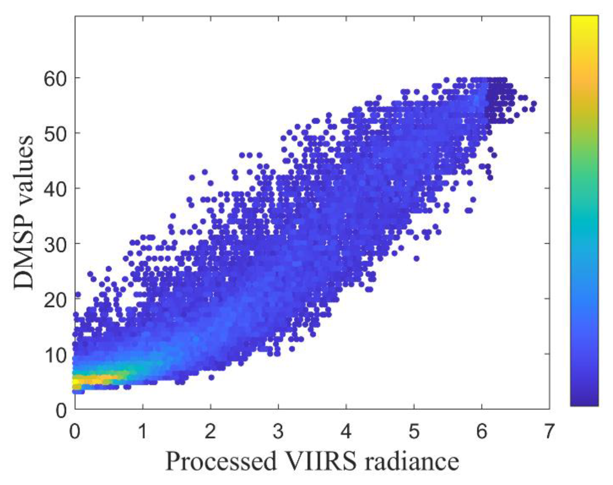
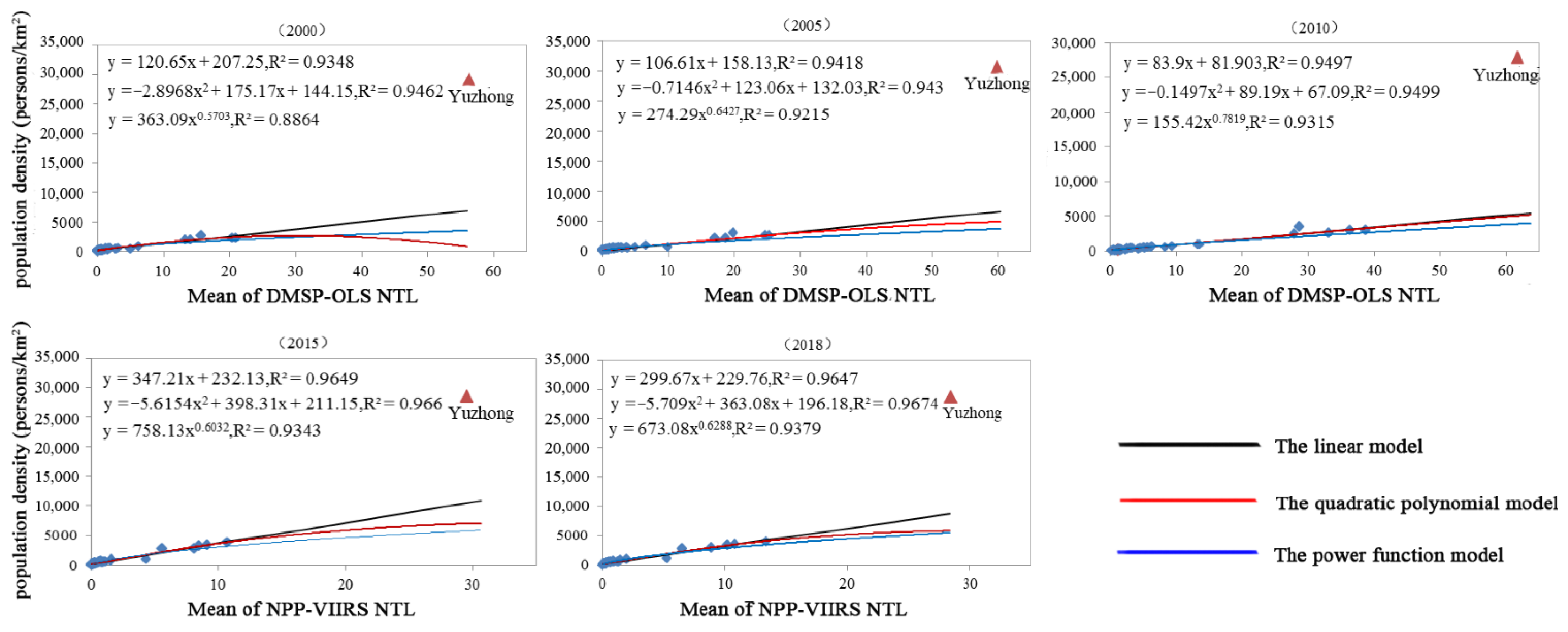
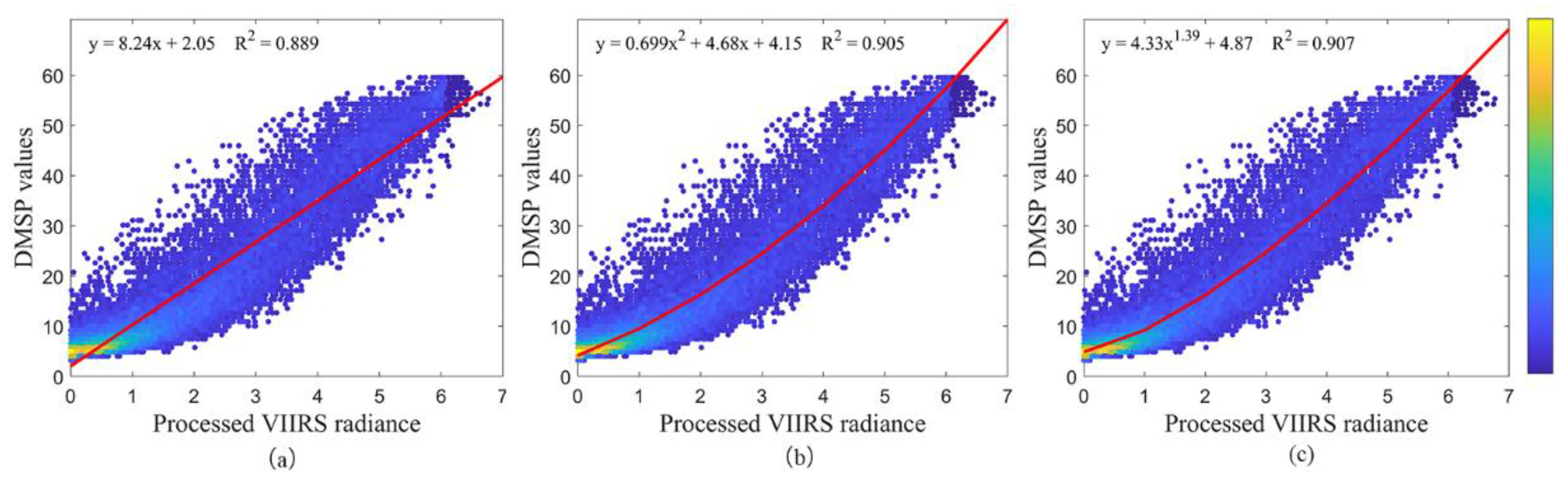
We integrated DMSP-OLS and NPP-VIIRS NTL data to construct a long-term NTL dataset, using the random-effect model with land-use data and corrected NTL data to model the spatiotemporal dynamics of the Chongqing’s population from 2000–2018. At the pixel level, there was a power function relationship between the two datasets (R2 = 0.907). Compared with an NTL integration model previously established at the provincial level, our model was 4.78% more accurate. In addition, accuracy tests using 2015 data resulted in an MRE of 26.98%, an improvement of nearly 20% when compared with previous studies of mountainous populations. Therefore, our approach is feasible and provides a technical method for monitoring spatiotemporal population changes in mountainous areas.
From 2000–2018, the spatial distribution of Chongqing’s population has increased in the west and decreased in the east, while also increasing in low-altitude areas and decreasing in the medium-high altitude areas. Moreover, population agglomeration was common. At the provincial level, high-density regions showed a significant increase, while decreasing in intermediate-density regions. The population density significantly increased in the central urban area and immediate surroundings in every district and county, while significantly decreased in non-urban areas, especially in the northeast.

Author Contributions

The co-authors together contributed to the completion of this article. Specifically, it follows their individual contribution: conceptualization, D.L. and Y.W.; data curation, H.Z., Y.W. and K.S.; formal analysis, Q.Y. and Y.W.; investigation, D.L. and Y.L.; methodology, D.L. and Y.W.; project administration, Q.Y.; writing—original draft, D.L.; writing—review and editing, D.L., Y.W. and Q.Y. All authors have read and agreed to the published version of the manuscript.

Funding

This research was funded by National Natural Science Foundation of China, grant number 42071234 and 41901232; Chongqing Social Science Planning Project, grant number 2019PY49; the Youth Fund for Humanities and Social Sciences Research of the Ministry of Education, grant number 19XJCZH006; and the Fundamental Research Funds for the Central Universities, grant number XDJK2020C014.

Institutional Review Board Statement

Not applicable.

Informed Consent Statement

Not applicable.

Data Availability Statement

Not applicable.

Conflicts of Interest

The authors declare no conflict of interest.

References

  1. Hu, H. The distribution of population in China, with statistics and maps. Acta Geogr. Sin. 1935, 2, 33–74. [Google Scholar]
  2. Grether, J.-M.; Mathys, N. Is the World’s economic centre of gravity already in Asia? Area 2010, 42, 47–50. [Google Scholar] [CrossRef]
  3. Quah, D. The global economy’s shifting centre of gravity. Glob. Policy 2011, 2, 3–9. [Google Scholar] [CrossRef]
  4. Powell, J.J.W. Comparative education in an age of competition and collaboration. Comp. Edu. 2020, 56, 57–78. [Google Scholar] [CrossRef] [Green Version]
  5. Zhang, Q.; Su, S. Determinants of urban expansion and their relative importance: A comparative analysis of 30 major metropolitans in China. Habitat Int. 2016, 58, 89–107. [Google Scholar] [CrossRef]
  6. Cai, H.; Yang, X.; Wang, K.; Xiao, L. Is forest restoration in the Southwest China Karst promoted mainly by climate change or human-induced factors? Remote Sens. 2014, 6, 9895–9910. [Google Scholar] [CrossRef] [Green Version]
  7. Liu, S.; Zhao, H.; Su, X.; Deng, L.; Dong, S.; Zhang, X. Spatio-temporal variability in rangeland conditions associated with climate change in the Altun mountain national nature reserve on the Qinghai-Tibet plateau over the past 15 years. Rangel. J. 2015, 37. [Google Scholar] [CrossRef]
  8. Xianfeng, L.; Zhu, X.; Pan, Y.; Shuangshuang, L.; Yuqi, M.; Juan, N. Spatiotemporal variation of vegetation coverage in Qinling-Daba mountains in relation to environmental factors. Acta Geogr. Sin. 2015, 70, 705–716. [Google Scholar] [CrossRef]
  9. Li, W.; Li, X.; Tan, M.; Wang, Y. Influences of population pressure change on vegetation greenness in China’s mountainous areas. Ecol. Evol. 2017, 7, 9041–9053. [Google Scholar] [CrossRef]
  10. Li, S.; Sun, Z.; Tan, M.; Li, X. Effects of rural–urban migration on vegetation greenness in fragile areas: A case study of Inner Mongolia in China. J. Geogr. Sci. 2016, 26, 313–324. [Google Scholar] [CrossRef] [Green Version]
  11. Lei, Z.; Dayong, Z. Relationship between ecological civilization and balanced population development in China. Energy Proced. 2011, 5, 2532–2535. [Google Scholar] [CrossRef] [Green Version]
  12. Wu, W.; Niu, S. Evolutional analysis of coupling between population and resource-environment in China. Proced. Environ. Sci. 2012, 12, 793–801. [Google Scholar] [CrossRef] [Green Version]
  13. Ryan, S.J.; Palace, M.W.; Hartter, J.; Diem, J.E.; Chapman, C.A.; Southworth, J. Population pressure and global markets drive a decade of forest cover change in Africa’s Albertine rift. Appl. Geogr. 2017, 81, 52–59. [Google Scholar] [CrossRef]
  14. Grau, H.R.; Aide, M. Globalization and land-use transitions in Latin America. Ecol. Soc. 2008, 13, 16. [Google Scholar] [CrossRef] [Green Version]
  15. Aide, T.M.; Clark, M.L.; Ricardo Grau, H.; Lopez-Carr, D.; Levy, M.A.; Redo, D.; Bonilla-Moheno, M.; Riner, G.; Andrade-Nunez, M.J.; Muniz, M. Deforestation and reforestation of Latin America and the Caribbean (2001–2010). Biotropica 2013, 45, 262–271. [Google Scholar] [CrossRef]
  16. Alahmadi, M.; Atkinson, P.; Martin, D. Estimating the spatial distribution of the population of Riyadh, Saudi Arabia using remotely sensed built land cover and height data. Comp. Environ. Urban Syst. 2013, 41, 167–176. [Google Scholar] [CrossRef]
  17. Azar, D.; Engstrom, R.; Graesser, J.; Comenetz, J. Generation of fine-scale population layers using multi-resolution satellite imagery and geospatial data. Remote Sens. Environ. 2013, 130, 219–232. [Google Scholar] [CrossRef]
  18. Hu, Y.; Wang, Q.; Liu, Y.; Li, J.; Ren, W. Index System and Transferring Methods to Build the National Society and Economy Grid atabase. J. Geo-Inf. Sci. 2011, 13, 573–578. [Google Scholar]
  19. Tan, M.; Li, X.; Li, S.; Xin, L.; Wang, X.; Li, Q.; Li, W.; Li, Y.; Xiang, W. Modeling population density based on nighttime light images and land use data in China. Appl. Geogr. 2018, 90, 239–247. [Google Scholar] [CrossRef]
  20. Tritsch, I.; Le Tourneau, F.-M. Population densities and deforestation in the Brazilian Amazon: New insights on the current human settlement patterns. Appl. Geogr. 2016, 76, 163–172. [Google Scholar] [CrossRef] [Green Version]
  21. Tan, M.; Li, X.; Lu, C.; Luo, W.; Kong, X.; Ma, S. Urban population densities and their policy implications in China. Habitat Int. 2008, 32, 471–484. [Google Scholar] [CrossRef]
  22. Zeng, C.; Zhou, Y.; Wang, S.; Yan, F.; Zhao, Q. Population spatialization in China based on night-time imagery and land use data. Int. J. Remote Sens. 2011, 32, 9599–9620. [Google Scholar] [CrossRef]
  23. Chowdhury, P.K.R.; Maithani, S.; Dadhwal, V.K. Estimation of urban population in Indo-Gangetic plains using night-time OLS data. Int. J. Remote Sens. 2012, 33, 2498–2515. [Google Scholar] [CrossRef]
  24. Yang, X.; Yue, W.; Gao, D. Spatial improvement of human population distribution based on multi-sensor remote-sensing data: An input for exposure assessment. Int. J. Remote Sens. 2013, 34, 5569–5583. [Google Scholar] [CrossRef]
  25. Hu, Y.; Zhao, G.; Zhang, Q. Spatial distribution of population data based on nighttime light and LUC data in the Sichuanchongqing region. J. Geo. Inform. Sci. 2018, 20, 68–78. [Google Scholar]
  26. Liu, Y.; Wang, J.; Wang, Z. Simulation of the spatial pattern of population of urban and rural residents in Huang-Huai-Hai area based on NPP/VIIRS nighttime lights. Areal Res. Develop. 2019, 38, 176–180. [Google Scholar]
  27. Wang, M.; Wang, J. Spatialization of township-level population based on nighttime light and land use data in Shandong province. J. Geo Inform. Sci. 2019, 21, 699–709. [Google Scholar]
  28. Sutton, P. Modeling population density with night-time satellite imagery and GIS. Comp. Environ. Urb. Syst. 1997, 21, 227–244. [Google Scholar] [CrossRef]
  29. Amaral, S.; Câmara, G.; Monteiro, A.M.V.; Quintanilha, J.A.; Elvidge, C.D. Estimating population and energy consumption in Brazilian Amazonia using DMSP night-time satellite data. Comp. Environ. Urb. Syst. 2005, 29, 179–195. [Google Scholar] [CrossRef]
  30. Zhou, Y.; Smith, S.J.; Elvidge, C.D.; Zhao, K.; Thomson, A.; Imhoff, M. A cluster-based method to map urban area from DMSP/OLS nightlights. Remote Sens. Environ. 2014, 147, 173–185. [Google Scholar] [CrossRef]
  31. Tian, Y.; Yue, T.; Zhu, L.; Clinton, N. Modeling population density using land cover data. Ecol. Model. 2005, 189, 72–88. [Google Scholar] [CrossRef]
  32. Wang, L.; Wang, S.; Zhou, Y.; Liu, W.; Hou, Y.; Zhu, J.; Wang, F. Mapping population density in China between 1990 and 2010 using remote sensing. Remote Sens. Environ. 2018, 210, 269–281. [Google Scholar] [CrossRef]
  33. Elvidge, C.; Baugh, K.; Zhizhin, M.; Hsu, F.-C. Why VIIRS data are superior to DMSP for mapping nighttime lights. Proc. Asia Pac. Adv. Netw. 2013, 35, 62–69. [Google Scholar] [CrossRef] [Green Version]
  34. Shi, K.; Chen, Y.; Yu, B.; Xu, T.; Yang, C.; Li, L.; Huang, C.; Chen, Z.; Liu, R.; Wu, J. Detecting spatiotemporal dynamics of global electric power consumption using DMSP-OLS nighttime stable light data. Appl. Energy 2016, 184, 450–463. [Google Scholar] [CrossRef]
  35. Zhao, M.; Zhou, Y.; Li, X.; Cao, W.; He, C.; Yu, B.; Li, X.; Elvidge, C.D.; Cheng, W.; Zhou, C. Applications of satellite remote sensing of nighttime light observations: Advances, challenges, and perspectives. Remote Sens. 2019, 11, 1971. [Google Scholar] [CrossRef] [Green Version]
  36. Small, C.; Elvidge, C.D.; Baugh, K. Urban Remote Sensing Event (JURSE), 2013 Joint. In Mapping Urban Structure and Spatial Connectivity with VIIRS and OLS Night Light Imagery, Urban Remote Sensing Event (JURSE); IEEE: New York, NY, USA, 2013; pp. 230–233. [Google Scholar]
  37. Zhao, M.; Zhou, Y.; Li, X.; Zhou, C.; Cheng, W.; Li, M.; Huang, K. Building a Series of Consistent Night-Time Light Data (1992–2018) in Southeast Asia by Integrating DMSP-OLS and NPP-VIIRS. IEEE Trans. Geosci. Remote Sens. 2020, 58, 1843–1856. [Google Scholar] [CrossRef]
  38. Zheng, Q.; Weng, Q.; Wang, K. Developing a new cross-sensor calibration model for DMSP-OLS and Suomi-NPP VIIRS night-light imageries. ISPRS J. Photogramm. Remote Sens. 2019, 153, 36–47. [Google Scholar] [CrossRef]
  39. Zhu, X.; Ma, M.; Yang, H.; Ge, W. Modeling the spatiotemporal dynamics of gross domestic product in China using extended temporal coverage nighttime light data. Remote Sens. 2017, 9, 626. [Google Scholar] [CrossRef] [Green Version]
  40. Shao, X.; Cao, C.; Zhang, B.; Qiu, S.; Elvidge, C.; Hendy, M. Radiometric calibration of DMSP-OLS sensor using VIIRS day/night band. Proc. SPIE Int. Soc. Opt. Eng. 2014, 9264. [Google Scholar] [CrossRef]
  41. Li, X.; Li, D.; Xu, H.; Wu, C. Intercalibration between DMSP/OLS and VIIRS night-time light images to evaluate city light dynamics of Syria’s major human settlement during Syrian civil war. Int. J. Remote Sens. 2017, 38, 5934–5951. [Google Scholar] [CrossRef]
  42. Yang, J.; Li, Y.; Wang, R. Sichuan and chongqing: Strategic fulcrum of the belt and road initiatives and Yangtze river economic zone. Reform Econ. Syst. 2015, 4, 58–64. [Google Scholar]
  43. Baugh, K.; Elvidge, C.; Tilottama, G.; Ziskin, D. Development of a 2009 stable lights product using DMSP-OLS data. Proc. Asia Pac. Adv. Netw. 2010, 30. [Google Scholar] [CrossRef]
  44. Xuecao, L.; Zhou, Y. A stepwise calibration of global DMSP/OLS stable nighttime light data (1992–2013). Remote Sens. 2017, 9, 637. [Google Scholar] [CrossRef] [Green Version]
  45. Elvidge, C.D.; Baugh, K.E.; Dietz, J.B.; Bland, T.; Sutton, P.C.; Kroehl, H.W. Radiance calibration of DMSP-OLS low-light imaging data of human settlements. Remote Sens. Environ. 1999, 68, 77–88. [Google Scholar] [CrossRef]
  46. Wu, R.; Yang, D.; Dong, J.; Zhang, L.; Xia, F. Regional inequality in China based on NPP-VIIRS night-time light imagery. Remote Sens. 2018, 10, 240. [Google Scholar] [CrossRef] [Green Version]
  47. Shi, K.; Yu, B.; Huang, Y.; Hu, Y.; Yin, B.; Chen, Z.; Chen, L.; Wu, J. Evaluating the ability of NPP-VIIRS nighttime light data to estimate the gross domestic product and the electric power consumption of China at multiple scales: A comparison with DMSP-OLS data. Remote Sens. 2014, 6, 1705–1724. [Google Scholar] [CrossRef] [Green Version]
  48. Tuan, Y.F. Geography, phenomenology, and the study of human nature. Can. Geogr./Le Geographe Canadien 1971, 15, 181–192. [Google Scholar] [CrossRef]
  49. Bright, E.A.; Rose, A.N.; Urban, M.L. LandScan 2015, 2015th ed.; Oak Ridge National Laboratory: Oak Ridge, TN, USA, 2016. [Google Scholar]
  50. Zhuo, L.; Zhang, X.; Zheng, J.; Tao, H.; Guo, Y. An EVI-based method to reduce saturation of DMSP/OLS nighttime light data. Acta Geogr. Sin. 2015, 70, 1339–1350. [Google Scholar]
  51. Kyba, C.; Kuester, T.; Sanchez de Miguel, A.; Baugh, K.; Jechow, A.; Hölker, F.; Bennie, J.; Elvidge, C.; Gaston, K.; Guanter, L. Artificially lit surface of Earth at night increasing in radiance and extent. Sci. Adv. 2017, 3, e1701528. [Google Scholar] [CrossRef] [Green Version]
Figure 1. Location map of the study area.
Remotesensing 13 00284 g001
Figure 2. Scatter density plots of DMSP and processed VIIRS nighttime lights (NTLs) in 2013.
Remotesensing 13 00284 g002
Figure 3. Relationship between light intensity and population density at the county level in Chongqing.
Remotesensing 13 00284 g003
Figure 4. Correlation between the Defense Meteorological Satellite Program (DMSP) and processed Visible Infrared Imaging Radiometer Suite (VIIRS) values at the pixel scale for the (a) linear model, (b) quadratic polynomial model and (c) power function model.
Remotesensing 13 00284 g004
Figure 5. Spatial distribution of the villages and towns selected.
Remotesensing 13 00284 g005
Figure 6. Simulated results of population density in Chongqing in 2000, 2005, 2010, 2015 and 2018.
Remotesensing 13 00284 g006
Figure 7. Changes in population density in Chongqing from 2000 to 2018.
Remotesensing 13 00284 g007
Figure 8. High-population-density regions in Chongqing in 2000 and 2018.
Remotesensing 13 00284 g008
Table 1. Correlation analysis between population and land-use type (by area).
Land UseCultivated LandForestGrass LandWaterResidential LandUnused Land
Correlation coefficient0.399 ***−0.311 ***−0.160 **0.471 ***0.577 ***0.180 **
Note: ** and *** are significantly different from zero at the 5% and 1% levels, respectively.
Table 2. Accuracy assessment of the NTL integrated data by county.
CountyMean NTL for DMSP-OLS DataMean NTL for Adjusted NPP-VIIRS DataRE (%)
Xiushan1.14 1.29 13.41
Youyang0.50 0.59 17.76
Jiangjin2.97 3.54 19.13
Nanchuan1.67 1.85 11.31
Yongchuan5.79 6.70 15.75
Pengshui0.47 0.45 −4.64
Wulong1.34 1.24 −7.43
Banan5.29 5.83 10.16
Qianjiang1.67 1.59 −4.70
Rongchang4.57 5.18 13.46
Bishan11.90 12.42 4.38
Dadukou37.05 38.42 3.70
Nan’an37.45 35.73 −4.58
Jiulongpo29.55 30.85 4.39
Yuzhong57.76 57.90 0.24
Jiangbei31.31 32.20 2.84
Shapingba36.30 35.14 −3.18
Fengdu1.07 1.15 7.55
Beibei14.65 14.40 −1.67
Changshou8.45 8.55 1.16
Shizhu0.92 0.98 5.48
Yubei14.95 14.98 0.20
Tongnan2.06 2.11 2.65
Tongliang5.50 5.59 1.69
Hechuan3.61 3.94 9.22
Dianjiang3.45 3.20 −7.34
Zhongxian1.43 1.47 2.51
Wanzhou2.94 2.66 −9.54
Liangping2.36 2.24 −5.17
Yunyang1.31 1.12 −15.00
Fengjie1.21 1.17 −3.32
Kaizhou1.52 1.50 −1.38
Wuxi1.59 1.18 −26.00
Wushan0.62 0.61 −2.29
Chengkou0.19 0.27 42.46
Fuling4.05 3.98 −1.73
Dazu5.60 6.11 9.09
Qijiang2.80 3.21 14.66
MRE(%)--8.19
Table 3. Estimated coefficients for the random-effect model.
VariableCoefficientStd. ErrorT Valuep > |t|
the NT of cultivated land0.00020.00021.470.142
the NT of forest−0.001 **0.000−2.190.028
the NL of residential land0.261 ***0.02311.540.000
the ND of cultivated land−0.0010.002−0.410.685
the ND of grassland0.0050.0031.450.147
the NPA of 0–300 m0.081 ***0.0194.300.000
the NPA of 300–500 m0.015 **0.0072.280.023
the NPA of 500–1000 m0.007 **0.0041.990.046
the NPA of >1000 m−0.010 **0.004−2.520.012
Con44.861 ***6.5016.900.000
Sigma_u15.474
Sigma_e5.842
Rho0.875
Note: (1) *, ** and *** are significantly different from zero at the 10%, 5% and 1% levels, respectively.
Table 4. Relative error (RE) classification for villages and townships.
RESeriously UnderestimatedGenerally UnderestimatedRelatively AccurateGenerally OverestimatedSeriously Overestimated
(−100% to −50%](−50% to −20%](−20% to 20%](20% to 50%](50% to −100%]
Number of villages and townships1230692712
Table 5. Changes in population density from 2000 to 2018.
Regional DivisionPopulation DensityLand Area (2000)Land Area (2005)Land Area (2010)Land Area (2015)Land Area (2018)
(persons/km2)(103 km2)(103 km2)(103 km2)(103 km2)(103 km2)
Low-density <5014.18 14.91 15.12 16.59 16.06
50–20021.46 22.43 24.53 25.50 25.01
Intermediate-density 200–50032.32 30.96 29.65 26.14 26.71
500–150012.71 12.24 10.82 11.52 11.67
High-density 1500–30000.80 0.85 0.97 1.14 1.16
>30000.27 0.35 0.65 0.84 1.12
Table 6. Average population density and total population of each altitude zone.
Regional DivisionMean Population Density (people/km2)Total Population (104 people)
2000200520102015201820002005201020152018
Low-altitude550.58554.00585.39626.88647.081829.081838.121944.312079.002145.08
Medium-altitude232.66227.09226.76227.34223.70685.90669.81665.13656.15645.57
High-altitude64.4560.9459.2958.0658.78113.65110.02102.6593.5295.46
Publisher’s Note: MDPI stays neutral with regard to jurisdictional claims in published maps and institutional affiliations.

