NPP-VIIRS DNB Daily Data in Natural Disaster Assessment: Evidence from Selected Case Studies

 , , and
Abstract
:
1. Introduction
2. Materials and Methods
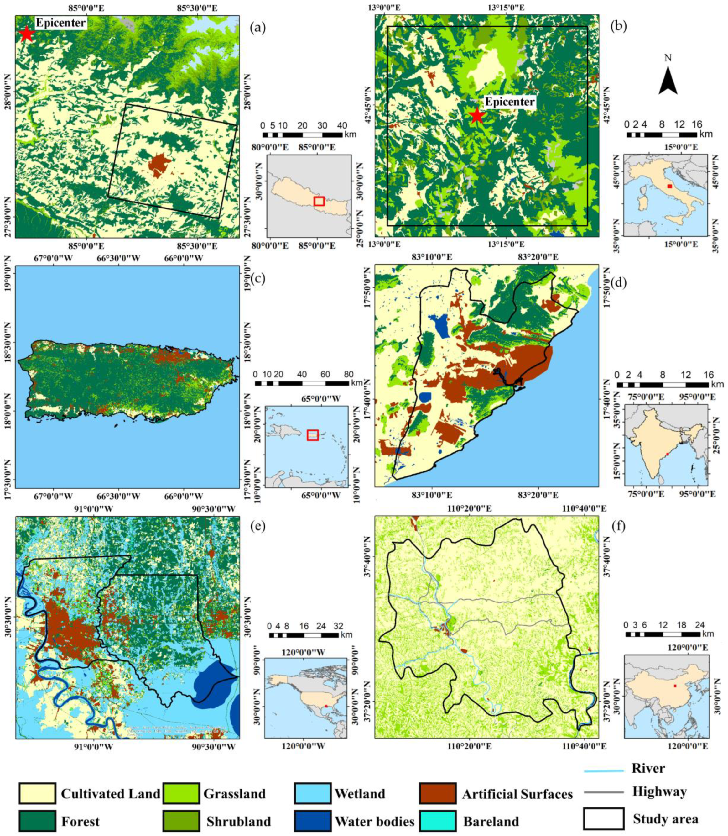
2.1. Event Selection
2.2. Data
2.3. Methods
2.3.1. Data Preprocessing
2.3.2. PNL Image
2.3.3. Statistical Significance
3. Results
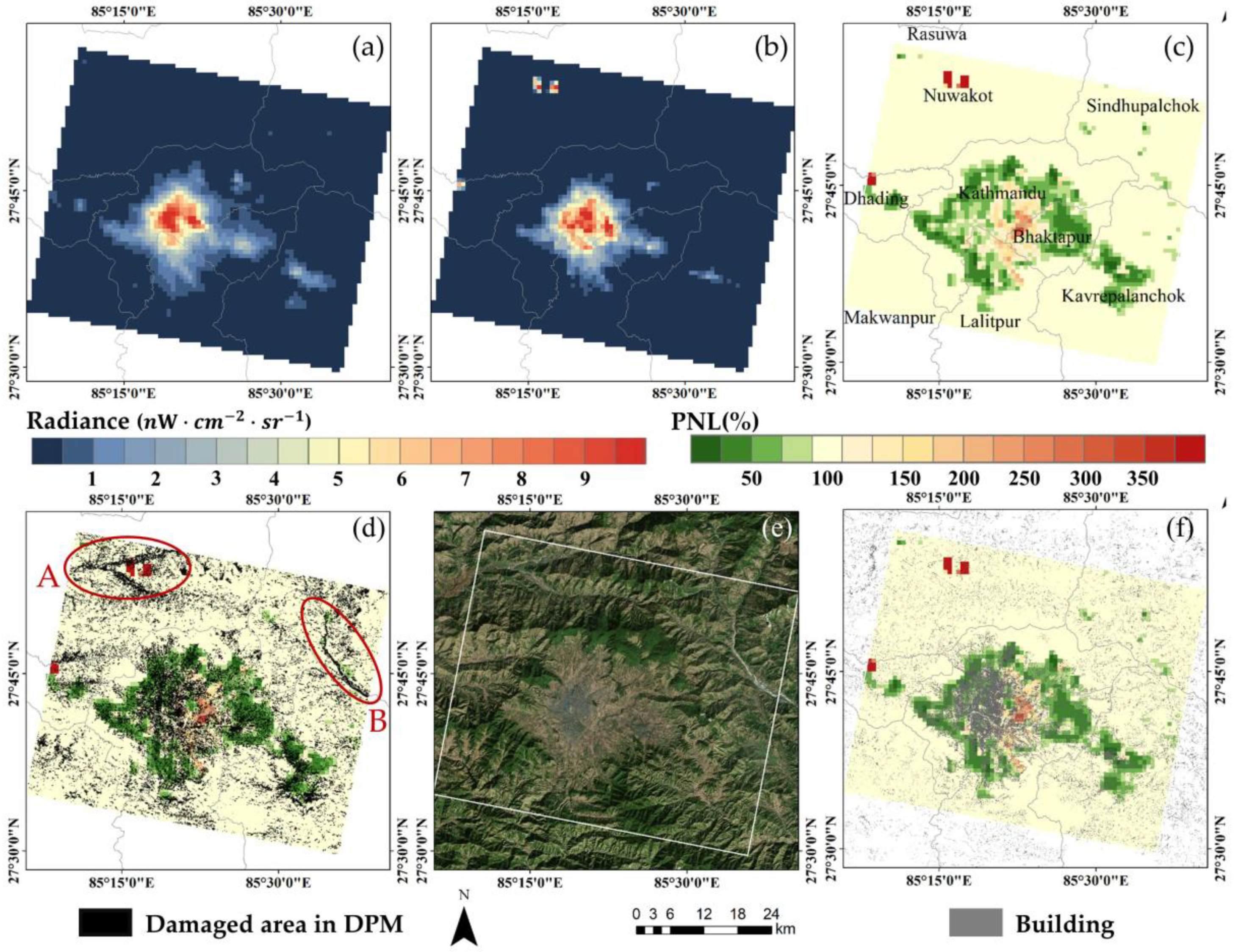
3.1. Earthquakes
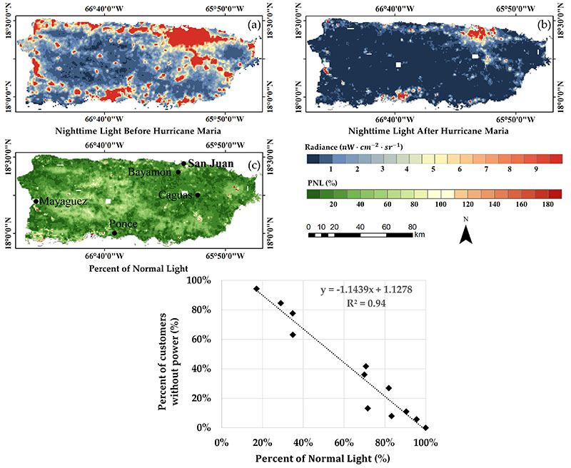
3.2. Storms
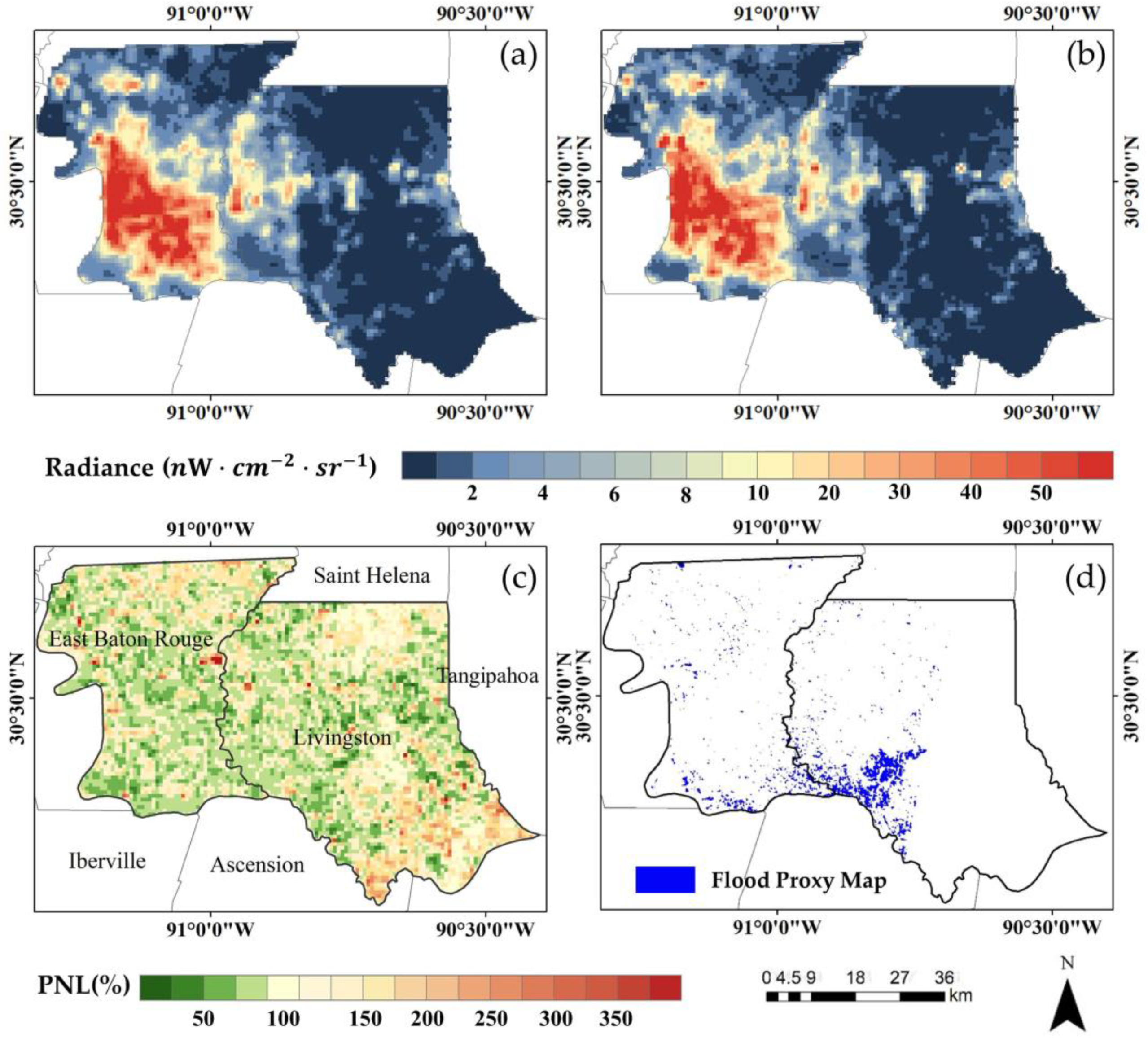
3.3. Floods
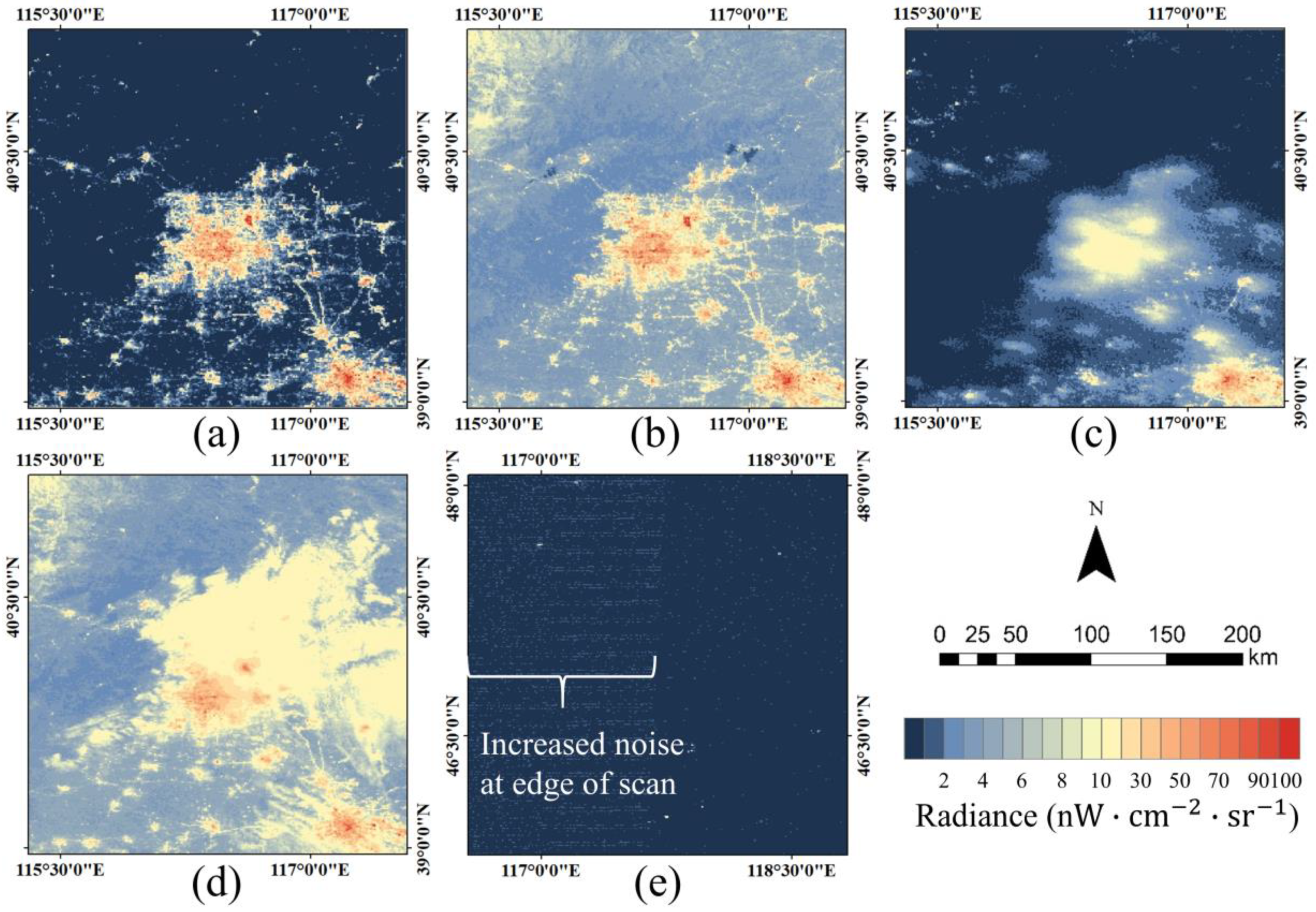
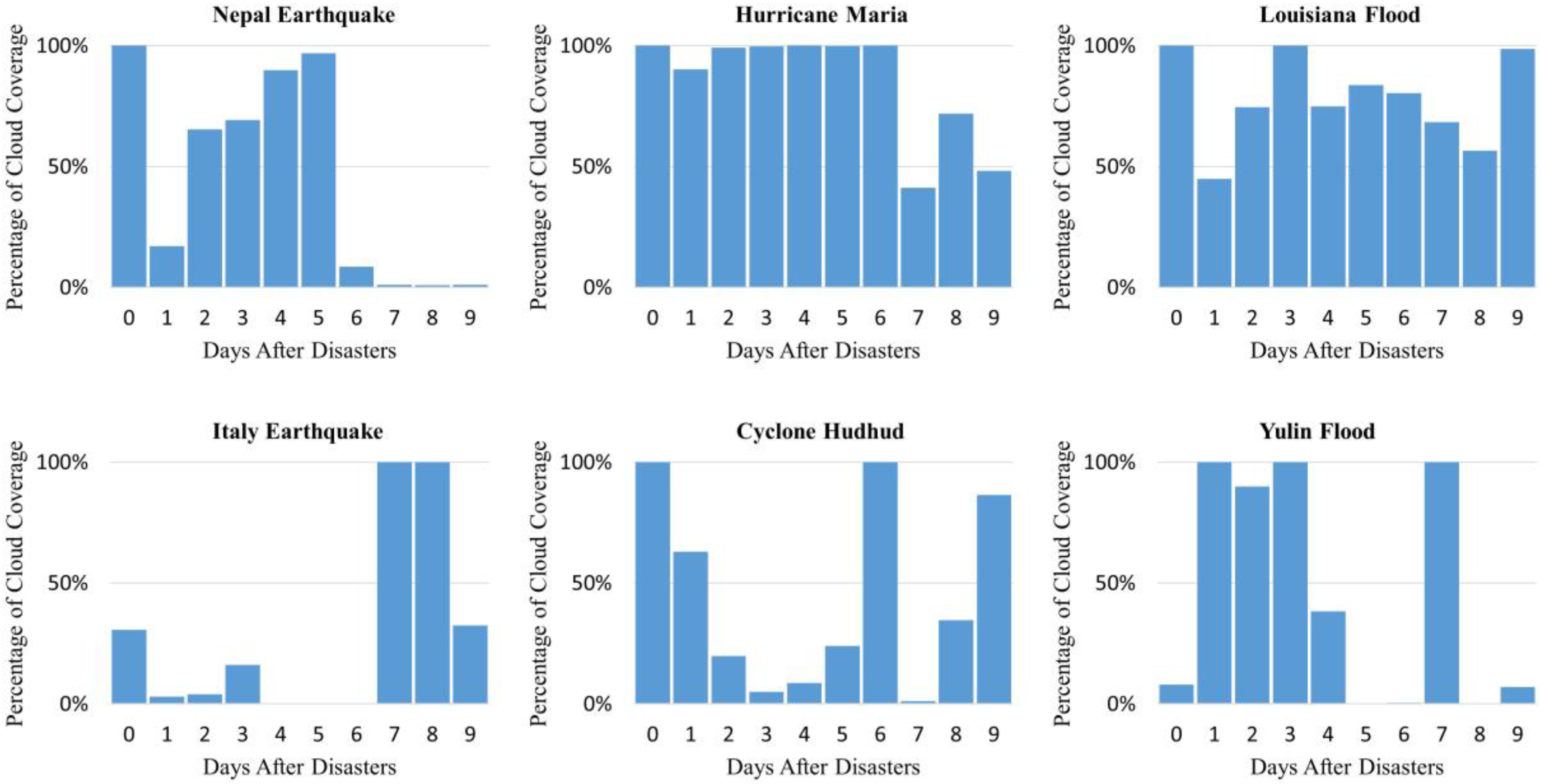
3.4. Impact of Clouds on Assessing Natural Disasters
4. Discussion
5. Conclusions
Author Contributions
Funding
Acknowledgments
Conflicts of Interest
References
- Soonee, S.; Narasimhan, S.; Nallarasan, N.; Rathour, H.K.; Yadav, G.; Bhan, S.; Mali, R. Impact of very severe cyclone ‘hudhud’on power system operation. In Proceedings of the 2015 Annual IEEE India Conference (INDICON), New Delhi, India, 17–20 December 2015; pp. 1–5. [Google Scholar] [CrossRef]
- Okamura, M.; Bhandary, N.P.; Mori, S.; Marasini, N.; Hazarika, H. Report on a reconnaissance survey of damage in Kathmandu caused by the 2015 Gorkha Nepal earthquake. Soils Found. 2015, 55, 1015–1029. [Google Scholar] [CrossRef]
- Klemas, V. Remote sensing of floods and flood-prone areas: An overview. J. Coast. Res. 2015, 314, 1005–1013. [Google Scholar] [CrossRef]
- Dell’Acqua, F.; Gamba, P. Remote sensing and earthquake damage assessment: Experiences, limits, and perspectives. Proc. IEEE 2012, 100, 2876–2890. [Google Scholar] [CrossRef]
- Dell’Acqua, F.; Bignami, C.; Chini, M.; Lisini, G.; Polli, D.A.; Stramondo, S. Earthquake damages rapid mapping by satellite remote sensing data: L’aquila April 6th, 2009 event. IEEE J. Sel. Top. Appl. Earth Obs. Remote. Sens. 2011, 4, 935–943. [Google Scholar] [CrossRef]
- Li, S.; Sun, D.; Goldberg, M.D.; Sjoberg, B.; Santek, D.; Hoffman, J.P.; DeWeese, M.; Restrepo, P.; Lindsey, S.; Holloway, E. Automatic near real-time flood detection using Suomi-NPP/VIIRS data. Remote. Sens. Environ. 2018, 204, 672–689. [Google Scholar] [CrossRef]
- Elvidge, C.D.; Baugh, K.E.; Kihn, E.A.; Kroehl, H.W.; Davis, E.R. Mapping city lights with nighttime data from the DMSP operational linescan system. Photogramm. Eng. Remote. Sens. 1997, 63, 727–734. [Google Scholar]
- Miller, S.D.; Straka, W.; Mills, S.P.; Elvidge, C.D.; Lee, T.F.; Solbrig, J.; Walther, A.; Heidinger, A.K.; Weiss, S.C. Illuminating the capabilities of the Suomi national polar-orbiting partnership (NPP) visible infrared imaging radiometer suite (VIIRS) day/night band. Remote. Sens. 2013, 5, 6717–6766. [Google Scholar] [CrossRef]
- Elvidge, C.D.; Cinzano, P.; Pettit, D.; Arvesen, J.; Sutton, P.; Small, C.; Nemani, R.; Longcore, T.; Rich, C.; Safran, J. The nightsat mission concept. Int. J. Remote. Sens. 2007, 28, 2645–2670. [Google Scholar] [CrossRef]
- Elvidge, C.D.; Baugh, K.; Zhizhin, M.; Hsu, F.C.; Ghosh, T. VIIRS night-time lights. Int. J. Remote. Sens. 2017, 38, 5860–5879. [Google Scholar] [CrossRef] [Green Version]
- Liao, L.B.; Weiss, S.; Mills, S.; Hauss, B. Suomi NPP VIIRS day-night-band (DNB) on-orbit performance. J. Geophys. Res. Atmos. 2013, 118, 705–718. [Google Scholar] [CrossRef]
- Shi, K.; Yu, B.; Huang, Y.; Hu, Y.; Yin, B.; Chen, Z.; Chen, L.; Wu, J. Evaluating the ability of NPP-VIIRS nighttime light data to estimate the gross domestic product and the electric power consumption of China at multiple scales: A comparison with dmsp-ols data. Remote. Sens. 2014, 6, 1705–1724. [Google Scholar] [CrossRef]
- Doll, C.N.H.; Muller, J.P.; Morley, J.G. Mapping regional economic activity from night-time light satellite imagery. Ecol. Econ. 2006, 57, 75–92. [Google Scholar] [CrossRef]
- Zhao, N.; Liu, Y.; Cao, G.; Samson, E.L.; Zhang, J. Forecasting China’s gdp at the pixel level using nighttime lights time series and population images. GISci. Remote. Sens. 2017, 54, 407–425. [Google Scholar] [CrossRef]
- Sutton, P.; Roberts, D.; Elvidge, C.; Baugh, K. Census from heaven: An estimate of the global human population using night-time satellite imagery. Int. J. Remote. Sens. 2001, 22, 3061–3076. [Google Scholar] [CrossRef]
- Sutton, P.; Roberts, C.; Elvidge, C.; Meij, H. A comparison of nighttime satellite imagery and population density for the continental United States. Photogramm. Eng. Remote. Sens. 1997, 63, 1303–1313. [Google Scholar]
- Elvidge, C.D.; Sutton, P.C.; Ghosh, T.; Tuttle, B.T.; Baugh, K.E.; Bhaduri, B.; Bright, E. A global poverty map derived from satellite data. Comput. Geosci. 2009, 35, 1652–1660. [Google Scholar] [CrossRef]
- Yu, B.L.; Shi, K.F.; Hu, Y.J.; Huang, C.; Chen, Z.Q.; Wu, J.P. Poverty evaluation using NPP-VIIRS nighttime light composite data at the county level in China. IEEE J. Sel. Top. Appl. Earth Obs. Remote. Sens. 2015, 8, 1217–1229. [Google Scholar] [CrossRef]
- Chand, T.R.K.; Badarinath, K.V.S.; Elvidge, C.D.; Tuttle, B.T. Spatial characterization of electrical power consumption patterns over India using temporal dmsp-ols night-time satellite data. Int. J. Remote. Sens. 2009, 30, 647–661. [Google Scholar] [CrossRef]
- He, C.; Ma, Q.; Li, T.; Yang, Y.; Liu, Z. Spatiotemporal dynamics of electric power consumption in Chinese mainland from 1995 to 2008 modeled using DMSP/OLS stable nighttime lights data. J. Geogr. Sci. 2012, 22, 125–136. [Google Scholar] [CrossRef]
- Shi, K.; Chen, Y.; Yu, B.; Xu, T.; Yang, C.; Li, L.; Huang, C.; Chen, Z.; Liu, R.; Wu, J. Detecting spatiotemporal dynamics of global electric power consumption using DMSP-OLS nighttime stable light data. Appl. Energy 2016, 184, 450–463. [Google Scholar] [CrossRef]
- Shi, K.; Chen, Y.; Yu, B.; Xu, T.; Chen, Z.; Liu, R.; Li, L.; Wu, J. Modeling spatiotemporal CO2 (carbon dioxide) emission dynamics in China from DMSP-OLS nighttime stable light data using panel data analysis. Appl. Energy 2016, 168, 523–533. [Google Scholar] [CrossRef]
- Ghosh, T.; Elvidge, C.D.; Sutton, P.C.; Baugh, K.E.; Ziskin, D.; Tuttle, B.T. Creating a global grid of distributed fossil fuel CO2 emissions from nighttime satellite imagery. Energies 2010, 3, 1895–1913. [Google Scholar] [CrossRef]
- Chen, Z.Q.; Yu, B.L.; Hu, Y.J.; Huang, C.; Shi, K.F.; Wu, J.P. Estimating house vacancy rate in metropolitan areas using NPP-VIIRS nighttime light composite data. IEEE J. Sel. Top. Appl. Earth Obs. Remote. Sens. 2015, 8, 2188–2197. [Google Scholar] [CrossRef]
- Hsu, F.-C.; Elvidge, C.D.; Matsuno, Y. Exploring and estimating in-use steel stocks in civil engineering and buildings from night-time lights. Int. J. Remote. Sens. 2013, 34, 490–504. [Google Scholar] [CrossRef]
- Shi, K.; Yu, B.; Hu, Y.; Huang, C.; Chen, Y.; Huang, Y.; Chen, Z.; Wu, J. Modeling and mapping total freight traffic in China using NPP-VIIRS nighttime light composite data. GISci. Remote. Sens. 2015, 52, 274–289. [Google Scholar] [CrossRef]
- Shi, K.; Chen, Y.; Yu, B.; Xu, T.; Li, L.; Huang, C.; Liu, R.; Chen, Z.; Wu, J. Urban expansion and agricultural land loss in China: A multiscale perspective. Sustainability 2016, 8, 790. [Google Scholar] [CrossRef]
- Li, X.; Li, D. Can night-time light images play a role in evaluating the syrian crisis? Int. J. Remote. Sens. 2014, 35, 6648–6661. [Google Scholar] [CrossRef]
- Li, X.; Zhang, R.; Huang, C.; Li, D. Detecting 2014 northern iraq insurgency using night-time light imagery. Int. J. Remote. Sens. 2015, 36, 3446–3458. [Google Scholar] [CrossRef]
- Levin, N.; Ali, S.; Crandall, D. Utilizing remote sensing and big data to quantify conflict intensity: The Arab Spring as a case study. Appl. Geogr. 2018, 94, 1–17. [Google Scholar] [CrossRef]
- Yu, B.; Tang, M.; Wu, Q.; Yang, C.; Deng, S.; Shi, K.; Peng, C.; Wu, J.; Chen, Z. Urban built-up area extraction from log-transformed NPP-VIIRS nighttime light composite data. IEEE Geosci. Remote. Sens. Lett. 2018, 1–5. [Google Scholar] [CrossRef]
- Shi, K.F.; Huang, C.; Yu, B.L.; Yin, B.; Huang, Y.X.; Wu, J.P. Evaluation of NPP-VIIRS night-time light composite data for extracting built-up urban areas. Remote. Sens. Lett. 2014, 5, 358–366. [Google Scholar] [CrossRef]
- Huang, Q.X.; Yang, X.; Gao, B.; Yang, Y.; Zhao, Y.Y. Application of dmsp/ols nighttime light images: A meta-analysis and a systematic literature review. Remote. Sens. 2014, 6, 6844–6866. [Google Scholar] [CrossRef]
- Elvidge, C.; Baugh, K.; Hobson, V.; Kihn, E.; Kroehl, H. Detection of fires and power outages using DMSP-OLS data. In Remote Sensing Change Detection: Environmental Monitoring Methods and Applications; Ross, S., Lunetta, C.D.E., Eds.; Taylor & Francis: London, UK, 1998; pp. 123–135. [Google Scholar]
- Molthan, A.; Jedlovec, G. Satellite observations monitor outages from superstorm sandy. Eos Trans. Am. Geophys. Union 2013, 94, 53–54. [Google Scholar] [CrossRef]
- Cole, T.; Wanik, D.; Molthan, A.; Román, M.; Griffin, R. Synergistic use of nighttime satellite data, electric utility infrastructure, and ambient population to improve power outage detections in urban areas. Remote. Sens. 2017, 9, 286. [Google Scholar] [CrossRef]
- Cao, C.; Shao, X.; Uprety, S. Detecting light outages after severe storms using the S-NPP/VIIRS day/night band radiances. IEEE Geosci. Remote. Sens. Lett. 2013, 10, 1582–1586. [Google Scholar] [CrossRef]
- Wang, Z.; Román, M.O.; Sun, Q.; Molthan, A.L.; Schultz, L.A.; Kalb, V.L. Monitoring disaster-related power outages using NASA black marble nighttime light product. Int. Arch. Photogramm. Remote. Sens. Spat. Inf. Sci. 2018, XLII-3, 1853–1856. [Google Scholar] [CrossRef]
- Kohiyama, M.; Hayashi, H.; Maki, N.; Higashida, M.; Kroehl, H.W.; Elvidge, C.D.; Hobson, V.R. Early damaged area estimation system using DMSP-OLS night-time imagery. Int. J. Remote. Sens. 2004, 25, 2015–2036. [Google Scholar] [CrossRef]
- Hayashi, H.; Matsuoka, M.; Fujita, H. Use of DMSP-OLS images for early identification of impacted areas due to the 1999 Marmara earthquake disaster. In Proceedings of the 20th Asian Conference on Remote Sensing, Hong Kong, China, 22–25 November 1999; pp. 1291–1296. [Google Scholar]
- Fan, X.; Nie, G.; Deng, Y.; An, J.; Zhou, J.; Li, H. Rapid detection of earthquake damage areas using VIIRS nearly constant contrast night-time light data. Int. J. Remote. Sens. 2018. [Google Scholar] [CrossRef]
- Roman, M.O.; Stokes, E.C. Holidays in lights: Tracking cultural patterns in demand for energy services. Earth Future 2015, 3, 182–205. [Google Scholar] [CrossRef] [PubMed] [Green Version]
- Agnew, J.; Gillespie, T.W.; Gonzalez, J.; Min, B. Baghdad nights: Evaluating the US military ‘surge’using nighttime light signatures. Environ. Plan. A 2008, 40, 2285–2295. [Google Scholar] [CrossRef]
- Emergency Events Database. Available online: http://emdat.be/emdat_db/ (accessed on 26 June 2018).
- Commission, N.P. Nepal Earthquake 2015: Post Disaster Needs Assessment. Vol. A: Key Findings; Government of Nepal, National Planning Commission: Kathmandu, Nepal, 2015. [Google Scholar]
- Italy in Shock after Amatrice Earthquake: This Used to Be My Home. Available online: https://www.theguardian.com/world/2016/aug/24/italy-earthquake-rescue-teams-dig-through-rubble-as-death-toll-rises (accessed on 26 June 2018).
- Amatrice (Italy) Earthquake Response. Available online: http://disastertechlab.org/2016/09/21/amatrice-italy-earthquake-response/ (accessed on 26 June 2018).
- In Pictures: Hurricane Maria Pummels Puerto Rico. Available online: http://edition.cnn.com/interactive/2017/09/world/hurricane-maria-puerto-rico-cnnphotos/ (accessed on 26 June 2018).
- Hurricane Maria Updates: In Puerto Rico, the Storm ‘Destroyed US’. Available online: https://www.nytimes.com/2017/09/21/us/hurricane-maria-puerto-rico.html (accessed on 26 June 2018).
- Hurricanes Nate, Maria, Irma, and Harvey Situation Reports. Available online: https://www.energy.gov/ceser/downloads/hurricanes-nate-maria-irma-and-harvey-situation-reports (accessed on 26 June 2018).
- Hudhud: Another Damaging Bay of Bengal Storm. Available online: https://earthobservatory.nasa.gov/IOTD/view.php?id=84547 (accessed on 26 June 2018).
- Cyclone Hudhud-Strategies and Lessons for Preparing Better & Strengthening Risk Resilience in Coastal Regions of India. Available online: https://ndma.gov.in/en/ndma-reports.html (accessed on 20 September 2018).
- Cyclone Hudhud Path and Affected Area Map. Available online: http://www.mapsofindia.com/mapinnews/cyclone-hudhud/ (accessed on 26 June 2018).
- August 2016 Record Flooding. Available online: https://www.weather.gov/lix/August2016flood (accessed on 26 June 2018).
- Thousands Still without Power; Many Will Have to Wait until Water Recedes, Officials Say. Available online: http://www.theadvocate.com/baton_rouge/news/weather_traffic/article_57ef9db6-633c-11e6-b19a-d7be27b1784b.html (accessed on 26 June 2018).
- Louisiana governor: 40K homes damaged by historic flooding, 11 killed. Available online: https://www.ctvnews.ca/world/louisiana-governor-40-000-homes-damaged-by-historic-flooding-11-killed-1.3030316 (accessed on 21 September 2018).
- He, Y.; He, S.; Hu, Z.; Qin, Y.; Zhang, Y. The devastating 26 July 2017 floods in Yulin city, northern Shaanxi, China. Geomat. Nat. Hazards Risk 2017, 9, 70–78. [Google Scholar] [CrossRef]
- The Flood in Suide, Shaanxi Province Have Affected 135,300 People and Caused Economic Losses of 2.265 Billion Yuan. Available online: http://www.jianzai.gov.cn//DRpublish/ztzl/0000000000025130.html (accessed on 26 June 2018).
- NOAA Comprehensive Large Array-Data Stewardship System (CLASS). Available online: https://www.bou.class.noaa.gov/saa/products/welcome (accessed on 9 March 2018).
- NASA EARTHDATA powered by the Earth Observing System Data and Information System (EOSDIS). Available online: https://earthdata.nasa.gov/ (accessed on 9 March 2018).
- NASA Jet Propulsion Laboratory Advanced Rapid Imaging and Analysis (ARIA) Project for Natural Hazards. Available online: https://aria.jpl.nasa.gov/ (accessed on 9 March 2018).
- Open Street Map. Available online: https://www.openstreetmap.org (accessed on 9 March 2018).
- GLOBELAND30. Available online: http://globallandcover.com/GLC30Download/index.aspx (accessed on 9 March 2018).
- GADM maps and data. Available online: https://gadm.org/ (accessed on 9 March 2018).
- Bai, Y.; Cao, C.Y.; Shao, X. Assessment of scan-angle dependent radiometric bias of Suomi-NPP VIIRS day/night band from night light point source observations. In Earth Observing Systems XX; Butler, J.J., Xiong, X., Gu, X., Eds.; Spie-Int Soc Optical Engineering: Bellingham, 2015; Vol. 9607. [Google Scholar]
- Hillger, D.; Seaman, C.; Liang, C.; Miller, S.; Lindsey, D.; Kopp, T. Suomi NPP VIIRS imagery evaluation. J. Geophys. Res. Atmos. 2014, 119, 6440–6455. [Google Scholar] [CrossRef]
- Cao, C.Y.; Bai, Y. Quantitative analysis of VIIRS DNB nightlight point source for light power estimation and stability monitoring. Remote. Sens. 2014, 6, 11915–11935. [Google Scholar] [CrossRef]
- Miller, S.D.; Turner, R.E. A dynamic lunar spectral irradiance data set for NPOESS/VIIRS day/night band nighttime environmental applications. IEEE Trans. Geosci. Remote. Sens. 2009, 47, 2316–2329. [Google Scholar] [CrossRef]
- Johnson, R.S.; Zhang, J.; Hyer, E.J.; Miller, S.D.; Reid, J.S. Preliminary investigations toward nighttime aerosol optical depth retrievals from the VIIRS day/night band. Atmos. Meas. Tech. 2013, 6, 1245–1255. [Google Scholar] [CrossRef]
- Schueler, C.F.; Lee, T.F.; Miller, S.D. Viirs constant spatial-resolution advantages. Int. J. Remote. Sens. 2013, 34, 5761–5777. [Google Scholar] [CrossRef]
- Levin, N. The impact of seasonal changes on observed nighttime brightness from 2014 to 2015 monthly viirs dnb composites. Remote. Sens. Environ. 2017, 193, 150–164. [Google Scholar] [CrossRef]
- Nachar, N. The Mann-Whitney U: A test for assessing whether two independent samples come from the same distribution. Tutor. Quant. Methods Psychol. 2008, 4, 13–20. [Google Scholar] [CrossRef]
- Pontius, R.G. Quantification error versus location error in comparison of categorical maps. Photogramm. Eng. Remote. Sens. 2000, 66, 1011–1016. [Google Scholar]
- Nearly Half a Million in Nepal Are Displaced from Their Homes; More Than 5,000 Dead. Available online: https://www.pri.org/stories/2015-04-25/devastating-earthquake-leaves-more-thousand-dead-and-rising-nepal (accessed on 13 August 2018).
- Italy Earthquake: Death Toll Rises to 267, Nearly 400 Hospitalised, Authorities Say. Available online: http://www.abc.net.au/news/2016-08-26/italy-quake-death-toll-rises-to-267-nearly-400-hospitalised/7789868 (accessed on 13 August 2018).
- Aftershocks Damage Access Routes to Earthquake-Damaged Village. Available online: http://www.irishnews.com/news/worldnews/2016/08/27/news/aftershocks-damage-access-routes-to-earthquake-damaged-village-669348/ (accessed on 13 August 2018).
- Hudhud Aftermath: Priority to Restore Power, Supply Essentials. Available online: http://www.thehindu.com/news/cities/Visakhapatnam/hudhud-aftermath-priority-to-restore-power-supply-essentials/article6503909.ece (accessed on 26 June 2018).
- Entergy Restores Power to Majority of Customers after Historic Flooding. Available online: http://www.tdworld.com/electric-utility-operations/entergy-restores-power-majority-customers-after-historic-flooding (accessed on 26 June 2018).
- A Dam Failure Warning Was Issued in Yulin, Shaanxi: The Reservoir Overflows and the Residents Need to Evacuate Immediately. Available online: http://news.china.com/domestic/945/20170726/31007133.html (accessed on 26 June 2018).
- Thieken, A.H.; Müller, M.; Kreibich, H.; Merz, B. Flood damage and influencing factors: New insights from the august 2002 flood in germany. Water Resour. Res. 2005, 41. [Google Scholar] [CrossRef]
- Colombia Landslide Leaves at Least 254 Dead and Hundreds Missing. Available online: https://www.theguardian.com/world/2017/apr/01/colombia-landslide-mocoa-putumayo-heavy-rains (accessed on 26 June 2018).
- Kerekes, J.P.; Strackerjan, K.; Salvaggio, C. Spectral reflectance and emissivity of man-made surfaces contaminated with environmental effects. Opt. Eng. 2008, 47, 106201. [Google Scholar] [CrossRef]
- Román, M.O.; Wang, Z.; Sun, Q.; Kalb, V.; Miller, S.D.; Molthan, A.; Schultz, L.; Bell, J.; Stokes, E.C.; Pandey, B.; et al. Nasa’s black marble nighttime lights product suite. Remote. Sens. Environ. 2018, 210, 113–143. [Google Scholar] [CrossRef]


| Disaster Type | Event | Time | Study Area |
|---|---|---|---|
| Earthquake | Gorkha Nepal Earthquake | 25 April 2015 06:11 a.m. (UTC) | Kathmandu and the surrounding area (Area size: 48 km × 57 km), Nepal |
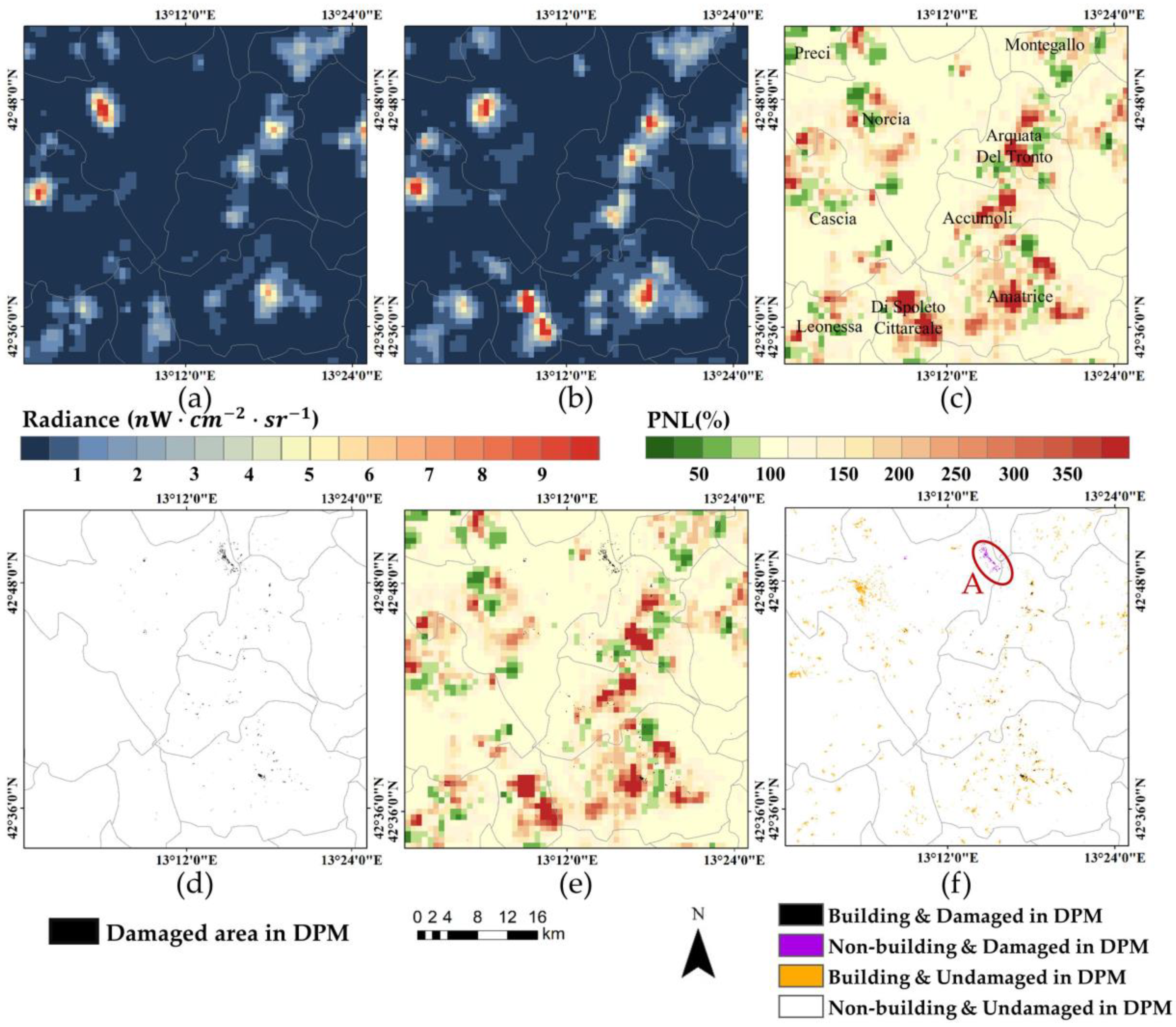
| Central Italy Earthquake | 24 August 2016 01:36 a.m. (UTC) | Accumoli, Amatrice, Norcia, and Arquata Del Tronto, Italy | |
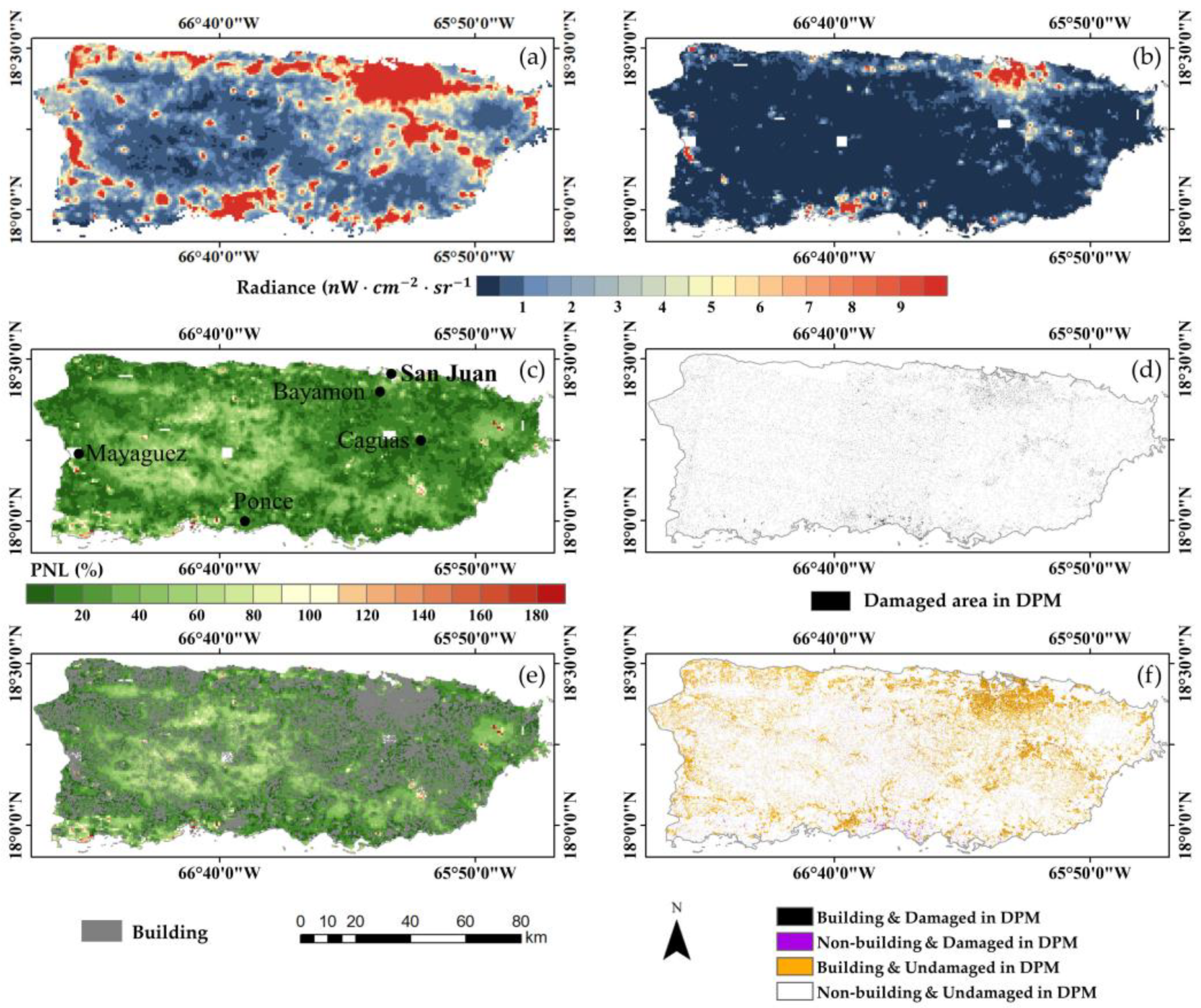
| Storm | Hurricane Maria | 20 September 2017 10:15 a.m. (UTC) | Puerto Rico, U.S. |
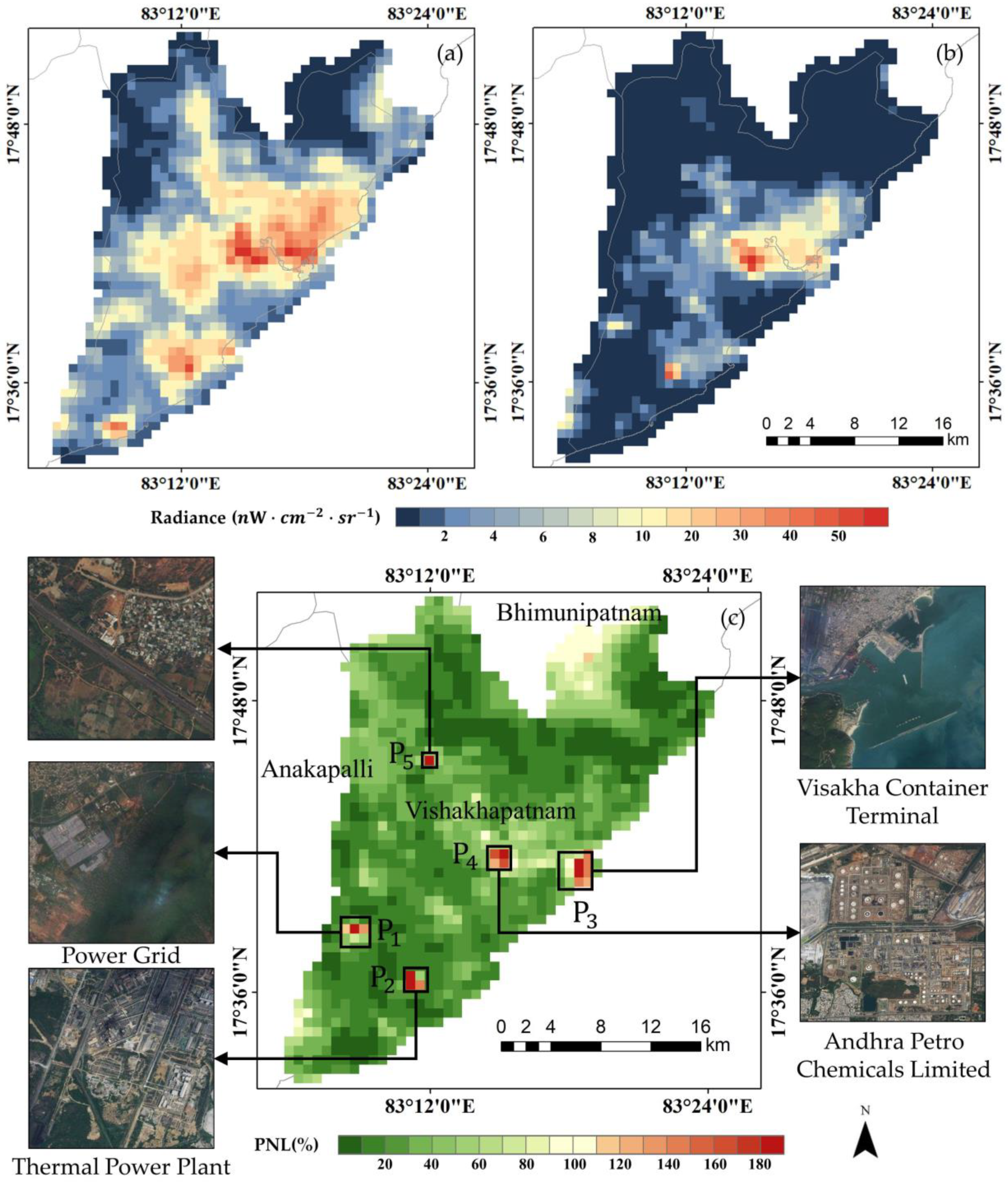
| Tropical Cyclone Hudhud | 12 October 2014 04:30 p.m. (UTC) | Visakhapatnam, India | |
| Flood | Louisiana Flood | 11 August 2016–16 August 2016 | East Baton Rouge Parish and Livingston Parish, U.S. |
| Yulin Flood | 25 July 2017–26 July 2017 | Suide, China |
| Pre-Earthquake | Post-Earthquake | |||||||||
|---|---|---|---|---|---|---|---|---|---|---|
| Date | 7April | 8 April | 9 April | 18 April | 21 April | 23 April | 26 April | 2 May | 4 May | 5 May |
| Days Before (After) the Disaster | 18 | 17 | 16 | 7 | 4 | 2 | 1 | 7 | 9 | 10 |
| Cloud Coverage (%) | 0.1 | 0.0 | 0.0 | 0.7 | 0.6 | 2.5 | 17.1 | 1.1 | 1.1 | 0.1 |
| Earthquake Event | Actual (DPM) | Predicted (NTL) | Accuracy | ||
|---|---|---|---|---|---|
| Damaged | Undamaged | Total | |||
| Gorkha Nepal Earthquake | Damaged | 488 | 871 | 1359 | Overall accuracy = 75.5% TPR = 35.9% FPR = 8.9% Kstandard = 0.31 Kquantity = 0.82 Klocation = 0.46 |
| (35.9%) | (64.1%) | ||||
| Undamaged | 307 | 3150 | 3457 | ||
| (8.9%) | (91.1%) | ||||
| Total | 795 | 4021 | |||
| Central Italy Earthquake | Damaged | 5 | 35 | 40 | Overall accuracy = 90.2% TRP = 12.5% FPR = 9.0% Kstandard = 0.01 Kquantity = 0.84 Klocation = 0.04 |
| (12.5%) | (87.5%) | ||||
| Undamaged | 322 | 3298 | 3620 | ||
| (8.9%) | (91.1%) | ||||
| Total | 327 | 3333 | |||
| Pre-Earthquake | Post-Earthquake | ||||||||||||
|---|---|---|---|---|---|---|---|---|---|---|---|---|---|
| Date | 4 August | 5 August | 8 August | 9 August | 11 August | 12 August | 13 August | 14 August | 15 August | 26 August | 27 August | 28 August | 30 August |
| Days Before (After) the Disaster | 20 | 19 | 16 | 15 | 13 | 12 | 11 | 10 | 9 | 2 | 3 | 4 | 6 |
| Cloud Coverage (%) | 5.5 | 4.6 | 4.0 | 12.3 | 0.0 | 0.0 | 2.1 | 15.6 | 21.9 | 4.0 | 16.1 | 0.0 | 0.0 |
| Study Area | Number of Buildings 1 | Total Population 2 | Average Number of People Per Building |
|---|---|---|---|
| Kathmandu and the surrounding area, Nepal | 220,451 | 3,566,322 | 16.2 |
| Four counties in Italy | 12,234 | 9371 | 0.8 |
| Pre-Storm | Post-Storm | |||||||||||
|---|---|---|---|---|---|---|---|---|---|---|---|---|
| Date | 22 August | 23 August | 24 August | 28 August | 30 August | 1 September | 18 September | 27 September | 28 September | 29 September | 7 October | 8 October |
| Days Before (After) the Disaster | 29 | 28 | 27 | 23 | 21 | 19 | 2 | 7 | 8 | 9 | 17 | 18 |
| Cloud Coverage (%) | 15.2 | 8.1 | 11.4 | 11.1 | 19.9 | 19.7 | 20.3 | 41.2 | 71.8 | 48.2 | 70.8 | 34.4 |
| Date Range | Dates of Available Image | Average DNB | PNL | Pnopower | |
|---|---|---|---|---|---|
| Before Storm | 20 August –20 September | 22 August–24 August, 28 August, 30 August, 1 September, 18 September | 4.52 | 0.0% | 0.0% |
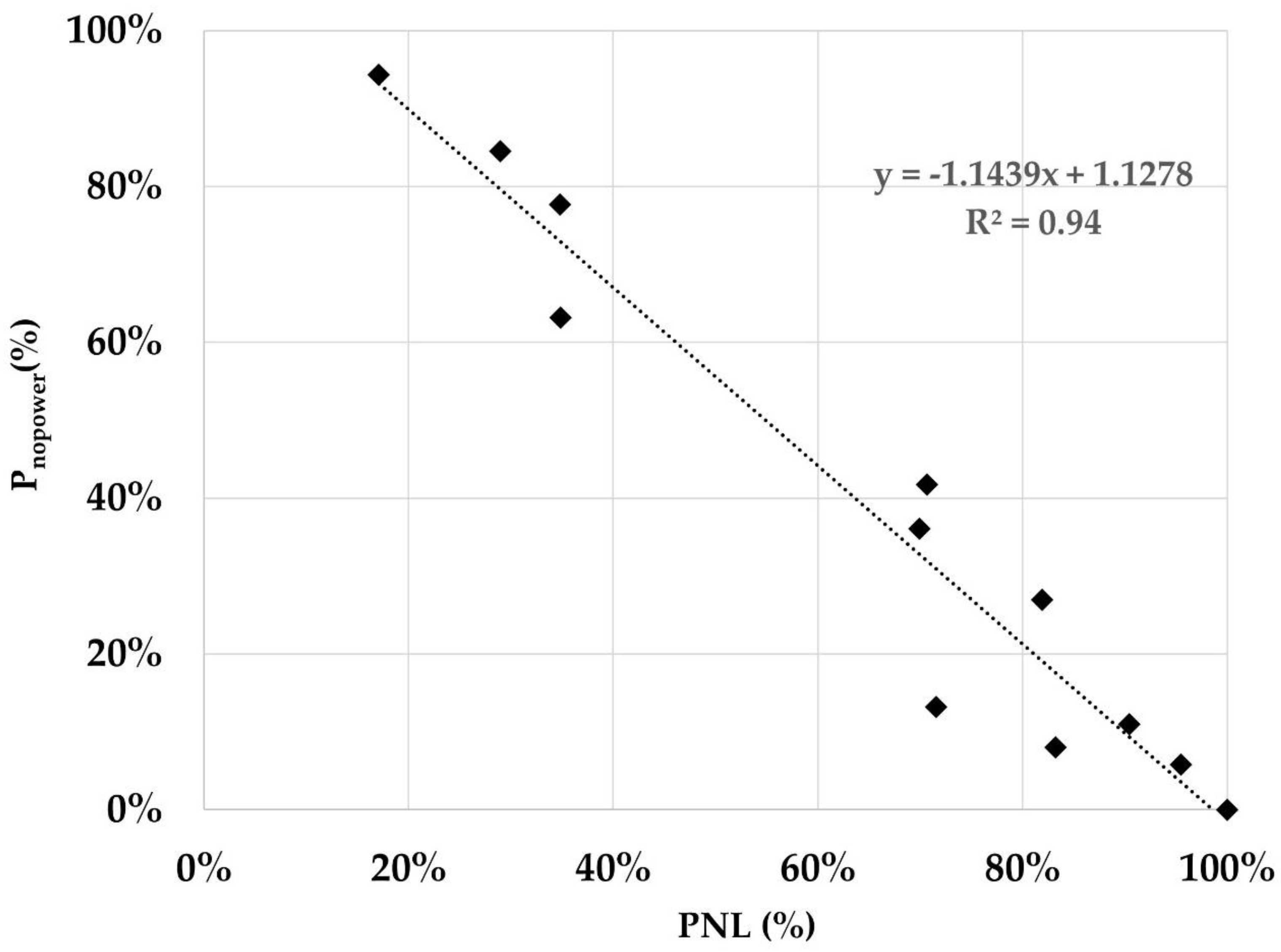
| After Storm | 21 September –10 October | 27 September –29 September, 7 October, 8 October | 0.77 | 17.1% | 94.3% |
| 11 October –20 October | 13 October, 15 October, 18 October, 19 October | 1.31 | 29.0% | 84.5% | |
| 21 October –30 October | 22 October –27 October | 1.57 | 34.8% | 77.7% | |
| 31 October –9 November | 31 October, 1 November, 3 November, 4 November | 1.58 | 34.9% | 63.1% | |
| 03 January –12 January | 3 January, 4 January, 10 January | 3.20 | 70.7% | 41.7% | |
| 13 January –22 January | 13 January –15 January, 18 January, 21 January, 22 January | 3.16 | 69.9% | 36.0% | |
| 23 January –1 February | 4 February, 9 February, 10 February, 11 February | 3.70 | 81.9% | 26.9% | |
| 22 February –3 March | 22 February –24 February, 27 February, 3 March | 3.24 | 71.6% | 13.2% | |
| 4 March –13 March | 4 March, 7 March, 11 March, 12 March, 13 March | 4.09 | 90.4% | 11.0% | |
| 14 March –23 March | 14 March, 15 March, 17 March, 19 March, 20 March | 3.76 | 83.2% | 7.6% | |
| 24 March –2 April | 24 March, 28 March | 4.32 | 95.5% | 5.8% |
| Pre-Storm | Post-Storm | ||||||
|---|---|---|---|---|---|---|---|
| Date | 27 September | 28 September | 29 September | 14 October | 15 October | 16 October | 19 October |
| Days Before (After) the Disaster | 15 | 14 | 13 | 2 | 3 | 4 | 7 |
| Cloud Coverage (%) | 15.6 | 6.6 | 0.0 | 19.8 | 4.9 | 8.6 | 1.2 |
| Pre-Flood | Post-Flood | |||||||||
|---|---|---|---|---|---|---|---|---|---|---|
| Date | 12 July | 13 July | 19 July | 22 July | 1 August | 2 August | 4 August | 21 August | 22 August | 24 August |
| Days Before (After) the Disaster | 30 | 29 | 23 | 20 | 10 | 9 | 7 | 10 | 11 | 13 |
| Cloud Coverage (%) | 0.0 | 0.0 | 9.0 | 0.0 | 19.9 | 0.0 | 5.6 | 22.7 | 21.3 | 0.0 |
| Pre-Flood | Post-Flood | ||||||
|---|---|---|---|---|---|---|---|
| Date | 27 June | 29 June | 1 July | 17 July | 30 July | 31 July | 2 August |
| Days Before (After) the Disaster | 29 | 27 | 24 | 8 | 4 | 5 | 7 |
| Cloud Coverage (%) | 12.7 | 0.0 | 1.2 | 0.7 | 0.0 | 0.5 | 0.0 |
| Disaster Type | Event | Application | Validation Data | Validation Results | Challenges |
|---|---|---|---|---|---|
| Earthquake | Gorkha Nepal Earthquake | Identify damaged areas | DPM | Overall accuracy = 75.5% TPR = 35.9% FPR = 8.9% Kstandard = 0.31 Kquantity = 0.82 Klocation = 0.46 | Rescue and repair activities produced extra lights |
| Central Italy Earthquake | None | DPM | Overall accuracy = 90.2% TPR = 12.5% FPR = 9.0% Kstandard = 0.01 Kquantity = 0.84 Klocation = 0.04 | Rescue and repair activities produced extra lights | |
| Storm | Hurricane Maria | Detect power outages | DPM, and Pnopower published by CESER in the U.S. | Strong correlation between the PNL and Pnopower (R2 = 0.94) | Cloud |
| Tropical Cyclone Hudhud | Detect power outages | Power outage rate in news reports | The estimated Pnopower of 77.6% was in good agreement with the report that 80% of the power supply was not restored. | Cloud | |
| Flood | Louisiana Flood | None | FPM and news reports | Mann-Whitney U-test indicates that the difference between pre- and post-flood images is not statistically significant | Cloud |
| Yulin Flood | Detect power outages | None | None | Increased rescue vehicles and repair activities brought extra lights |
© 2018 by the authors. Licensee MDPI, Basel, Switzerland. This article is an open access article distributed under the terms and conditions of the Creative Commons Attribution (CC BY) license (http://creativecommons.org/licenses/by/4.0/).
Share and Cite
Zhao, X.; Yu, B.; Liu, Y.; Yao, S.; Lian, T.; Chen, L.; Yang, C.; Chen, Z.; Wu, J. NPP-VIIRS DNB Daily Data in Natural Disaster Assessment: Evidence from Selected Case Studies. Remote Sens. 2018, 10, 1526. https://doi.org/10.3390/rs10101526
Zhao X, Yu B, Liu Y, Yao S, Lian T, Chen L, Yang C, Chen Z, Wu J. NPP-VIIRS DNB Daily Data in Natural Disaster Assessment: Evidence from Selected Case Studies. Remote Sensing. 2018; 10(10):1526. https://doi.org/10.3390/rs10101526
Chicago/Turabian StyleZhao, Xizhi, Bailang Yu, Yan Liu, Shenjun Yao, Ting Lian, Liujia Chen, Chengshu Yang, Zuoqi Chen, and Jianping Wu. 2018. "NPP-VIIRS DNB Daily Data in Natural Disaster Assessment: Evidence from Selected Case Studies" Remote Sensing 10, no. 10: 1526. https://doi.org/10.3390/rs10101526