Nighttime Lights and Population Migration: Revisiting Classic Demographic Perspectives with an Analysis of Recent European Data

Department of Sociology, Quinnipiac University, Hamden, CT 06518, USA
Remote Sens. 2020, 12(1), 169; https://doi.org/10.3390/rs12010169
Submission received: 27 November 2019
/
Revised: 30 December 2019
/
Accepted: 31 December 2019
/
Published: 3 January 2020
(This article belongs to the Special Issue Advances in Remote Sensing with Nighttime Lights)
Abstract
:This study examines whether the Visible Infrared Imaging Radiometer Suite (VIIRS) nighttime lights can be used to predict population migration in small areas in European Union (EU) countries. The analysis uses the most current data measured at the smallest administrative unit in 18 EU countries provided by the European Commission. The ordinary least squares regression model shows that, compared to population size and gross domestic product (GDP), lights data are another useful predictor. The predicting power of lights is similar to population but it is much stronger than GDP per capita. For most countries, regression models with lights can explain 50–90% of variances in small area migrations. The results also show that the annual VIIRS lights (2015–2016) are slightly better predictors for migration population than averaged monthly VIIRS lights (2014–2017), and their differences are more pronounced in high latitude countries. Further, analysis of quadratic models, models with interaction effects and spatial lag, shows the significant effect of lights on migration in the European region. The study concludes that VIIRS nighttime lights hold great potential for studying human migration flow, and further open the door for more widespread application of remote sensing information in studying dynamic demographic processes.
1. Introduction
The applications of nighttime lights in social science studies have flourished since the early 2000s, when nighttime light-based imagery data become available online [1,2,3,4]. Yet, its application in demographic studies are limited. Most applications of nighttime lights concentrate on the simple estimation of total population or population density [5,6]. In comparison, the field of economics uses lights data more receptively, probably due to the popular assumption that economic activities at night need electric lights, which can be detected by sensor-equipped satellites from space [3,4,7,8]. As a result, many studies focus on testing lights as an indicator of static population accounts, or as a predictor of economic output, or their related phenomena (such as urban extent or pollution). Interestingly, the variables most closely correlated with the brightness of light—population size, population density, and GDP—also inherently influence demographic processes. The goal of this study is to test the possibility that nighttime lights can be used to predict population migration flows. The study also examines how the lights–migration association fares against population–migration and GDP–migration associations in the process of revisiting classic demographic approaches to population migration. If the results of associations are similar, lights can be an effective migration predictor when population or GDP are not available, as lights have advantages of being available for the entire globe, updated timely, and versatile to aggregation by different geographic units.
Demography is a discipline that focuses on studying the causes and effects of population processes, which include migration, fertility, and mortality [9,10]. The most influential theoretical framework on human migration was formed around the mid-1900s, and generalized the common causes of migration, keying in on population size and economic conditions in place of origin and destinations [9]. Still a dominate theoretical perspective, including population size, density, and economic variables as underlying causes of migration flows is now normative in demographic research. Researchers routinely use population size and gross domestic product (GDP) variables in models to predict migration population size [11,12,13]. Data collection of these classic predictors rely heavily on traditional demographic data-gathering methods, including censuses, surveys, or government statistical reports [11,12]. As accurate population or GDP statistics in small areas are often unavailable through traditional data-gathering methods [4,14,15], migrations occurring in small areas, such as counties or towns, are difficult to predict. With fine resolution, imagery data gathered from remote sensors offer a novel data source to study human migration. Utilizing current and available European data in small areas—Nomenclature of Territorial Units for Statistics level III region (NUTS III)—this study is the first attempt to test whether lights can be a useful predictor for migration. The European Union statistical office provides detailed migration, population, and economic statistics in very small areas for many countries. Yet, such information is not available in other parts of the world. This makes the European Union (EU) data a good fit for testing the association between lights and migration and comparing their relationship with population and economic indicators. Such analysis can potentially help migration-related policy-making processes and allocating resources at the local level based on migrants’ needs.
2. Materials and Methods
2.1. Theoretical Background
In the field of demography, the migration process includes internal migration, which refers to movement within the same country, and international migration, which refers to movement across countries [9,10]. Based on the characteristics of migrants, migration can also be classified into marriage and settlement migration, regional and international labor migration, circulation migration, and refugees and forced migration [9,10]. Most migration processes in human history are voluntary [9].
Early generalizations about migration were set forth by E.G. Ravenstein during the late 1800s. Known as the “Laws of Migration” [16], they were mostly derived from empirical observations, such as “most migrations are over a short distance”, “migrations often occurs in steps”, “long-range migrations are usually to urban areas”, “most migrants are adults”, “large towns grow more by migration than birth rate”, and “migration increases with economic development”. During the 1900s, theoretical attempts to understand migration mechanics gained popularity. An early example of this was the gravity model of migration. Based on Newton’s law of gravity, it proposed that the populations of sending and receiving places could be viewed as analogous to mass in studies of physics. The larger the population of two places, and the closer the two places are in physical distance, the more migration we can expect to occur between the two places [17,18]. By the mid-twentieth century, push and pull factors were integrated into the framework to explain migrations [19]. The push factors at the place of origin and pull factors at the destination were widely defined, ranging from employment opportunities, income-generating opportunities, and the general state of the economy, to climate, safety, and educational opportunities. For example, we can consider a low employment rate as a push factor, pushing residents out to other places to find jobs, while a mild climate in a destination can be viewed as a pull factor, attracting more populations to reside there.
Since the twentieth century, economic models have gradually gained a dominant position in migration theories. There are multiple renditions of economic explanations of migration, including neoclassical economics [20], dual labor market theories [21], and household-based migration decisions [22]. All of them are based on a common assumption; that is, the larger the expected economic gain at destinations compared to the place of origin, the more power it has in influencing migration decisions and behaviors.
Based on these classic theories, population size/density and general economic measures of destinations, often derived from GDP or GDP per capita, are used as common predictors of migration in most empirical studies on migration. The general argument is that larger populations or a stronger economy attract more migrants, both internal and international migrants. Depending on the topic of individual research, other variables, such as government policy, immigration laws, culture, language, geography, and physical environment, are hypothesized and tested. Again, these predictors are typically treated as time- or region-specific manners.
The production of nighttime lights data in recent years has resulted in an uptick of empirical studies focusing on application of lights in understanding human settlement and economic activities. Among the applications of nighttime lights to demographic studies, most have examined the relationship between nighttime lights and population counts or density [23,24,25]. These studies found that nighttime lights have moderate to strong correlation with regional or country level populations. There are, however, very limited studies that investigate lights and dynamic population processes, such as fertility, mortality, or migration. Outliers to the general trend include studies using lights to verify European population decline as a result of low fertility rates [26], studies predicting infant mortality level in Chinese counties [27,28], and studies mapping refugee populations in Africa and the Middle East [29].
The most extensive application of nighttime lights appears in the field of economics. Rigorous statistical models were developed over the last decade using lights to predict national and regional GDP and income [2,30,31,32]. These studies found that the relationship between lights and economic statistics vary by region and countries and that lights are a more reliable predictor for cross sectional than time series analysis [33]. In addition, nighttime lights are also used to predict development-related phenomena, such as urban extent and CO2 emission [34,35,36].
With the recent advent of nighttime lights data to study human populations and their economic activities, most research confirms the close connection between lights and population and general economic statistics. What must now be confirmed is whether or not lights can be further used to understand and predict dynamic population processes, such as migration, other than static population mass or the state of economic development. This study is the first to inquire whether nighttime light captures local attributes that explain migration across small areas, and whether the association between nighttime lights and migration are comparable to the association between population size or GDP and migration. The following analysis will use updated VIIRS lights to predict migration population in the EU and compare the results with the results of population and economic predictors.
2.2. Data and Methods
Geographic boundaries, demographic and economic statistics used in this analysis were downloaded from the Eurostat database. Eurostat is the statistical office of the EU, providing the most updated and reliable statistics that enable comparisons between countries and regions of the EU. For statistical purposes, the EU classifies subregions within EU countries into three levels. This analysis uses Nomenclature of Territorial Units for Statistics level III region (NUTS III), which contains the smallest administrative regions of EU countries. For instance, there are around 100 NUTS III regions in France and about 400 NUTS III regions in Germany. The samples are selected from the most current classification (NUTS year 2016), which specifies 1348 regions at the NUTS III level. These regions cover all EU member states as well as European Free Trade Association (EFTA) countries. Switzerland is excluded because its regional economic data are not available. Countries with less than 15 NUTS III regions, such as Luxembourg, Denmark, and Slovenia are also excluded from the analysis, as the small sample size can result in unreliable regression estimates. The total NUTS III regions used in the following analysis without missing values are 1256 from 18 countries.
One way to measure migration population is migration flows. It considers the number of migrants entering and leaving (inflow and outflow) a country/region over a specific time period, typically one year. Eurostat measures this concept with net migration, which is the difference between the number of immigrants and the number of emigrants from a NUTS III region during a year. When the number of emigrants exceeds the number of immigrants, net migration is negative. In some cases, the numbers of immigrants and emigrants cannot be accurately estimated due to the lack of official or government records. This situation could happen to EU countries, since EU citizens can travel and move freely across EU country borders. To reduce estimation errors of net migration, Eurostat reports the net migration plus statistical adjustments at the NUTS III level. The adjusted net migration is based on the difference between population change and natural change starting 1 January for two consecutive years. That is, it combines information from the difference between inward and outward migration as well as other changes in the population which cannot be attributed to births, deaths, immigration or emigration. Total population and GDP per capita data are also downloaded from Eurostat. According to Eurostat, “total population” is measured with the “usually resident population,” which represents the number of inhabitants of a given area on 1 January of the year in question. GDP per capita is measured with purchasing power standard (PPS) per inhabitant at current market prices. The area size of regions is measured in square kilometers. Total population, GDP per capita, and area size are all measured at the NUTS III level.
The Earth Observations Group (EOG) at The National Oceanic and Atmospheric Administration (NOAA)/National Centers for Environmental Information (NCEI) produces the annual and monthly VIIRS composites [37]. This analysis uses VIIRS lights rather than stable lights, as VIIRS sensors generate higher quality images [38,39,40]. Further, VIIRS lights have better predictability than stable lights for both population and economic accounts [33]. The VIIRS monthly composites are available from April 2012 to the present, while the annual composites are available for 2015 and 2016. The process of generating annual VIIRS composites filters out temporal lights, such as those from aurora, fires, boats, and other background noises [40]. The monthly composites do not filter out these noises. Thus, we can expect that annual VIIRS composites have better results in predicting trends and patterns of population processes than monthly VIIRS composites. A very recent study suggests that annual composites have a stronger correlation with annual economic accounts than averaged monthly composites [30]. Since net migration is calculated at an annual basis, the following analysis reports the results of the annual composite first, and then compares this to the results of averaged monthly lights from 2014 to 2017. All lights data are aggregated to the NUTS III level using administrative unit maps from 2016.
The analyses use ordinary least squares regression and spatial lag models. The dependent variable is net migration population, and the independent variables include nighttime lights, total population, and GDP per capita. All variables are measured at the NUTS III level. Areas size is controlled in all regression models. In the models that include multiple years or multiple countries, year and country dummy variables are also included in the analysis.
3. Results
Table 1 reports the pairwise Pearson’s correlation coefficients and the number of observations used in the analysis. Net migration correlates with VIIRS lights variables, GDP per capita as well as population size. All coefficients are significant at p = 0.05 level, and have a similar magnitude, ranging from 0.11 to 0.300. Compared to annual VIIRS lights 2015 and 2016, averaged monthly VIIRS lights show a weaker correlation with migration, GDP per capita, and population, but a stronger correlation with area size. The two lights variables are not perfectly correlated (r = 0.78). This is probably due to the different processes of generating annual and monthly VIIRS lights. Both annual and monthly lights show a moderate correlation with population (r ranges from 0.45 to 0.74), but a fairly weak correlation with GDP per capita (0.014 to 0.045).
Considering that the EU has over twenty countries, and these countries vary by government policies, geographic location, and cultural and historical background, this study will first examine the small area migration for 18 large EU countries individually, comparing the effect of lights with the effects of population and GDP. Then, this study will examine the model with interaction effects, and the nonlinear and spatial lag models for the European region.
Classic migration theory suggests that places having higher GDP per capita and more population tend to attract more migrants. The ordinary least square (OLS) regression results suggest that such reasoning may not be applicable to all countries (Table 2). The estimated beta coefficients allow us to compare results across samples and models. For instance, the coefficient of GDP per capita indicates standard deviation increases in net migration for one standard deviation increase in GDP per capita. Table 2 shows that the economic pull factor, GDP per capita, significantly predicts migration in only six EU countries: Croatia, Finland, Italy, Netherlands, Spain, and the UK. The magnitude of the coefficient of GDP is relatively small, except for Croatia. In Finland, Netherlands, Spain, and UK, one standard deviation increase in GDP per capita only increases net migration population by less than 0.20 standard deviation. Population size of NUTS III area has significant, positive effects in the following countries: Austria, Finland, Germany, Netherlands, Spain, Sweden, and the UK. More importantly, the magnitude of the population’s effect is much larger than the GDP. The coefficient of population for several countries is close to 1.0, suggesting one standard deviation increase in population can lead to about one standard deviation increase in net migration population.
Annual lights are expected to have a positive effect on net migration, similar to population and GDP. Table 2 shows that this is the case for Belgium, Bulgaria, France, Greece, Hungary, Norway, Poland, and Romania. For these countries where lights have significant effects, the magnitude of these effects are also quite large and comparable to the effect of population size. The coefficient of lights is slightly weak for France (0.29) and Norway (0.40), but substantially stronger for Hungary (5.55).
To summarize, the analysis by country suggests that neither GDP pull factor nor population gravity effect can explain migration for all countries. For many EU countries, GDP per capita and population have negative effects on net migration, which run opposite of theoretical predications. VIIRS nighttime lights significantly predict net migration population for as many countries, but, just like GDP and population variables, they cannot significantly predict migration population for some countries tested. Overall, coefficients of lights and population are larger than GDP for most counties.
The above results indicate that lights, GDP per capita, and population can predict migration. However, testing all three variables in one model makes the interpretation of coefficients difficult, as lights correlate with population and GDP for certain countries. Regression estimates with multicollinearity are still BLUE (best linear unbiased estimators), but the estimated coefficients can have larger standard errors. A preliminary analysis shows that lights have small to moderate correlations with GDP per capita in almost all countries, except for annual VIIRS lights in Bulgaria and Romania. Yet, for 10 out of 18 countries tested, lights are highly correlated with population (r > 0.80). These countries include Austria, Belgium, Bulgaria, Croatia, France, Germany, Hungary, Italy, Portugal, Romania, and Spain. To address the collinearity issue in interpreting coefficient estimates, this study will test VIIRS lights and population in separate models for all countries.
Table 3 and Table 4 report separate analysis for VIIRS lights and population. Table 3 uses VIIRS annual lights and pooled data from 2015 and 2016. Table 4 uses VIIRS averaged monthly lights. There are more observations for each country in averaged monthly lights analysis, as this lights product is available from 2014 to 2017. GDP per capita for 2017 is only available for Belgium, Bulgaria, Hungary, and the UK. Thus, only analysis of those four countries include data up to 2017. For the remaining countries, the analysis uses data from 2014 to 2016. Year dummy variables are also included in the model to control unobserved yearly differences, but are not reported in the tables.
Compared to the results in population models (Table 3), the coefficients of VIIRS annual lights are significant in predicting net migration for 13 countries. That is, one country more than population models. The magnitude of the coefficient of lights is similar to that of population, which is above 0.5 for most countries. This means that for one standard deviation increase in lights, the net migration increases by at least 0.5 standard deviation. The difference between lights and population models is large for Belgium, the Netherlands and Romania. For Belgium, lights variable has more explanatory power than population. For the Netherlands, population explains migration much better than lights. For Romania, annual lights data have a positive, significant effect, but population has a negative effect. The variance in net migration can be explained by the data, and the lights model and population model show similar results. That is, for most countries, lights or population can explain 50–90% of variances in migration.
The coefficient of averaged monthly VIIRS lights is similar to that of annual VIIRS lights for most countries, and just slightly weaker for a few countries (Table 4). However, for Finland, Norway, and Sweden, the coefficients of averaged monthly lights are noticeably smaller than that of annual data. This suggests that filtering out background noises in processing annual lights results in different statistical outcomes, particularly for countries at higher latitudes.
Compared to the effects of lights and population, GDP has less consistent results across all countries. For about half of the countries tested, GDP per capita has a negative effect on migration. This is different from the hypothesis of classic demographic theories. For countries where the coefficient of GDP is significant, its magnitude is small, except for the countries of Croatia, Finland, Italy, and the Netherlands, where the coefficient of GDP is consistent and moderate. Overall, GDP per capita is a less important factor in predicting migration for most countries compared to population and lights.
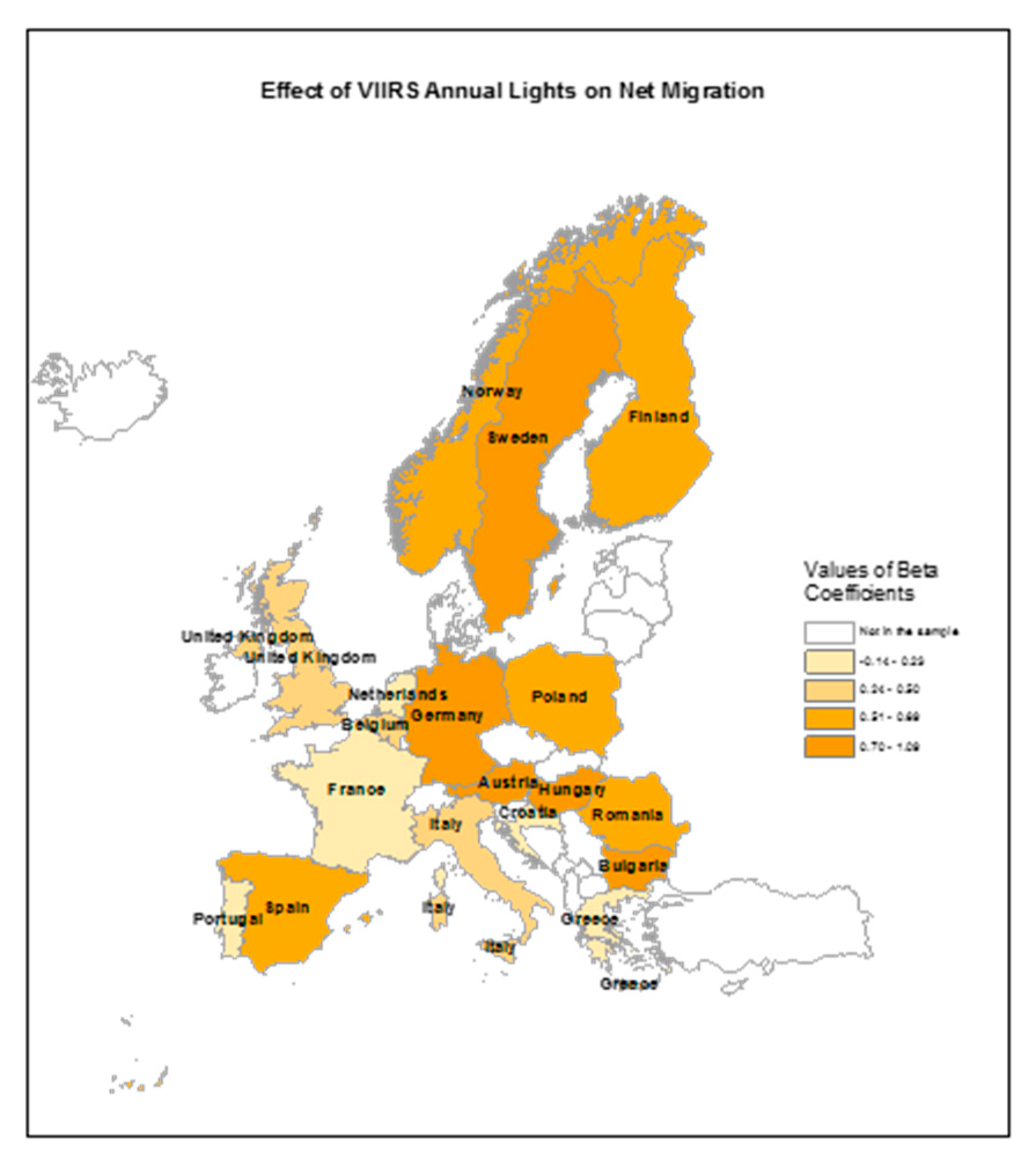
It is worth noting here that there is no obvious geographic pattern indicating where lights are more or less useful in explaining migration. Figure 1 illustrates the coefficients of lights by countries based on annual lights analysis (Table 3). The category with the lowest value of coefficients (–0.14 to 0.23) highlights countries for which lights cannot significantly predict migration populations. These countries, including the Netherlands, France, Portugal, Croatia, and Greece, are scattered throughout Europe. In Northern Europe, the lights variable has a relatively stronger effect on net migration. Yet, in Central, Western, and Southern Europe the effect of lights is mixed. In short, there is little evidence to suggest a clear geographical pattern of usefulness of nighttime lights in predicting migration.
The regression results of combined data from 18 countries with lights interaction terms also reveal the varying effect of lights on migration across countries. Table 5 shows the effects of interaction terms between lights and GDP, lights and population, and lights and country dummy variables. The significant coefficients suggest that lights’ effect on migration varies by population and GDP per capita. Hungary is used as a reference in the model to test lights’ varying effects across EU countries. Results in Table 2 and Table 3 suggest that the effect of lights is larger in Hungary than in most other EU countries. Lights variable has a significant, positive effect on migration at the base level. Most interaction terms between lights and country dummy variables are also significant, and with a negative sign, thus confirming lights’ varying effects across countries and that the magnitude of its effect is smaller in most countries than in Hungary.
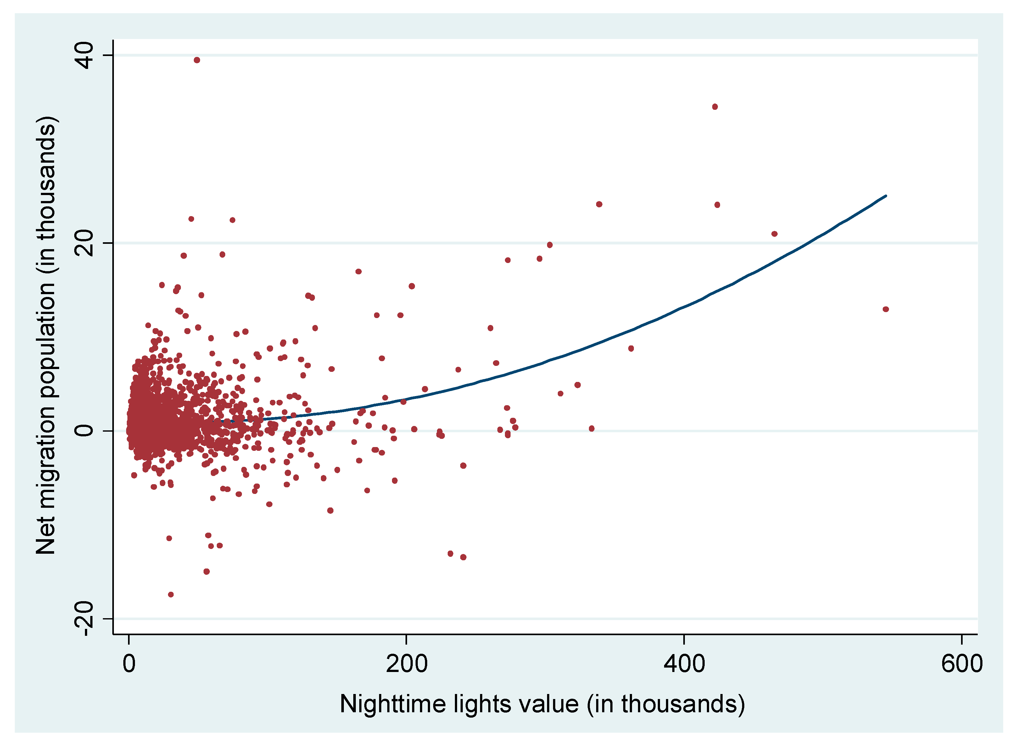
Finally, this study uses a quadratic model to test the non-linear relationship between migration and lights, and a spatial regression model to test the effect of lights under the assumption of spatial autocorrelation. These results are compared to the results of the linear model. All three models (Table 6) show the significant effects of lights on migration. The general model fit indicators suggest that the quadratic and spatial lag models fit the data better than the linear model. Figure 2 illustrates the quadratic relationship between the net migration size and nighttime lights values of NUTS III areas in EU countries. The spatial lag model assumes that migration population observed at one location is correlated with migration population of the neighboring areas or attributes of neighboring areas. The spatial lag model can capture the effect of surrounding areas, or the migration spillover effect. In such models, the spatial parameter q is estimated for the migration population of surrounding areas. The standardized spatial weight matrix, W, is the first order queen continuity weight matrix. The parameters in the spatial lag model are estimated with the maximum likelihood method.
Moran’s I statistics indicate that a spatial model is preferred over the linear OLS regression. Shown in Table 6, the estimated coefficients of lights, GDP per capita, and population are similar in OLS as in the spatial lag model. Most importantly, lights have a positive, significant effect on migration in both OLS and the spatial lag models. Furthermore, the spatial lag parameter q is also significant, thus showing that spatial dependence of the data should be considered when we study migration in small areas. Log likelihood and robust Lagrange multiplier (LM) test index indicate that the spatial lag model is preferred over linear OLS as well.
The sample is NUTS III areas of 18 EU countries used in this study. The migration and nighttime lights are the values of the year 2006.
4. Discussion
There are several important findings in this analysis. First, in general, VIIRS nighttime lights are useful in predicting migration population. Compared to population size and GDP, the two variables hypothesized within classic demographic theories, lights-based variables have more predicting power for very small regions in many European countries. This result not only presents in individual country analysis, but also is confirmed with the combined country sample and the spatial regression model. The effect of lights on migration is similar to that of population size, but much stronger than that of GDP for many countries. Second, annual lights and averaged monthly lights show slightly different results for most countries in Europe, but their differences are more pronounced in Northern European countries. Countries in high latitude regions, such as Iceland and Finland, can be influenced by aurora lights, therefore the different filtering processes in generating VIIRS lights products influence their statistical results. Researchers need to be cautious in selecting lights series in empirical analyses, especially when high latitude regions are among the sample tested. Third, in individual country analysis, neither GDP nor population had a consistent, positive effect on migration as theories suggested, nor did lights. There exist large variations across countries in how these variables can be used to predict migration flows. This is probably because at first, migration is such a dynamic phenomenon that no set of common variables provide equal explanation on migration for all countries. Government policies, history, location, natives’ sentiments, and other unique factors can also affect migration. Second, there are wide cultural differences and different patterns in light use across countries. This is well documented in light pollution literature and other light-based studies [41,42,43]. Thus, to understand migrations in local areas, particularly regarding their relationship with lights and GDP, it is important to examine data specific to a country. Fourth, there is no obvious geographic pattern indicating where lights data are more or less useful. Across Europe, from Bulgaria to Germany, from Austria to Sweden, lights variable is a strong predictor of migration flow for many countries, but also insignificant for others. Finally, the significant effect of lights appears in linear, quadratic, and spatial lag models. In comparison, quadratic model and spatial lag model fit the data better than the linear model. This suggests more advanced models, including nonlinear and spatial effect, are needed in future studies about migration. In addition, with the longer time series data, especially the long time series in high quality lights gathered over time, future studies need to examine the growth patterns of migration, which will help migration forecasts and population projections.
5. Conclusions
Nighttime lights data from remote sensing presents a novel approach to social science disciplines. Studies repeatedly show that nighttime lights correlate with GDP and population, but their correlations are not perfect, nor consistent across regions. This implies that nighttime lights capture or reflect other attributes of locality other than static population size or general economic output. For many European countries, nighttime lights are more useful in predicting migration flow than predictors proposed by classic demographic theories. The possible explanation is that migration process is a such dynamic process, influenced by culture, history, different industry sectors, local amenities, infrastructure, and other factors. The classic demographic perspective emphasizes a general measure on population size and GDP, but these variables may not capture other local attributes that help explain migration. Nighttime lights, on the other hand, may reflect some of those attributes. Thus, although lights are not a direct driving force of migration, they can be used to predict migration better than population size or GDP for certain countries.
Migration not only determines population, gender structure, and racial and ethnicity makeup, but also relates to other demographic processes, including fertility, mortality, and population growth. Classic demographic theories are still relevant today, but new data based on nighttime lights present additional opportunities to expand conventional explanations. With its advantage of being scaled to small areas and updated monthly, nighttime lights has potential to identify and track the dynamic demographic process better than other social or economic predictors in some regions. This will help policy makers to allocate resource or adjust local policy according to migrants’ needs in a timely fashion. This study demonstrates that, in addition to estimates of static population or economic statistics, lights data can further our understanding about more dynamic, fluid population processes, such as human migration, and it opens a door for further applications of remote sensing information in demographic studies.
Funding
This research received no external funding.
Acknowledgments
I thank my colleague Keith Kerr for helping with the preparation of this paper.
Conflicts of Interest
The author declares no conflict of interest.
References
- Elvidge, C.D.; Sutton, P.C.; Ghosh, T.; Tuttle, B.T.; Baugh, K.E.; Bhaduri, B.; Bright, E. A global poverty map derived from satellite data. Comput. Geosci. 2009, 35, 1652–1660. [Google Scholar] [CrossRef]
- Ghosh, T.; LPowell, R.; DElvidge, C.; EBaugh, K.; CSutton, P.; Anderson, S. Shedding light on the global distribution of economic activity. Open Geogr. J. 2010, 3, 147–160. [Google Scholar]
- Henderson, J.V.; Storeygard, A.; Weil, D.N. Measuring economic growth from outer space. Am. Econ. Rev. 2012, 102, 994–1028. [Google Scholar] [CrossRef] [PubMed] [Green Version]
- Chen, X.; Nordhaus, W.D. Using luminosity data as a proxy for economic statistics. Proc. Natl. Acad. Sci. USA 2011, 108, 8589–8594. [Google Scholar] [CrossRef] [Green Version]
- Lo, C.P. Modeling the population of China using DMSP operational linescan system nighttime data. Photogramm. Eng. Remote Sens. 2001, 67, 1037–1047. [Google Scholar]
- Sutton, P.C.; Elvidge, C.; Obremski, T. Building and Evaluating Models to Estimate Ambient Population Density. Photogramm. Eng. Remote Sens. 2003, 69, 545–553. [Google Scholar] [CrossRef]
- Keola, S.; Andersson, M.; Hall, O. Monitoring Economic Development from Space: Using Nighttime Light and Land Cover Data to Measure Economic Growth. World Dev. 2015, 66, 322–334. [Google Scholar] [CrossRef]
- Doll, C.N.; Muller, J.-P.; Morley, J.G. Mapping regional economic activity from night-time light satellite imagery. Ecol. Econ. 2006, 57, 75–92. [Google Scholar] [CrossRef]
- Anderson, B. World Population Dynamics: An Introduction to Demography. In Chapter 12: Migration and Urbanization; Pearson: Upper Saddle River, NJ, USA, 2014; pp. 402–458. [Google Scholar]
- Weeks, J. Population: An Introduction to Concepts and Issues; Thomason Higher Education: Belmont, CA, USA, 2008. [Google Scholar]
- White, M.J.; Lindstrom, D.P. Internal migration. In Handbook of Population; Springer: Boston, MA, USA, 2005; pp. 311–346. [Google Scholar]
- Brown, S.K.; Bean, F.D. International migration. In Handbook of Population; Springer: Boston, MA, USA, 2005; pp. 347–382. [Google Scholar]
- Karemera, D.; Oguledo, V.I.; Davis, B. A gravity model analysis of international migration to North America. Appl. Econ. 2000, 32, 1745–1755. [Google Scholar] [CrossRef]
- Ghosh, M.; Rao, J.N.K. Small Area Estimation: An Appraisal. Stat. Sci. 1994, 9, 55–76. [Google Scholar] [CrossRef]
- Williamson, P.; Birkin, M.; Rees, P.H. The estimation of population microdata by using data from small area statistics and samples of anonymised records. Environ. Plan. A Econ. Space 1998, 30, 785–816. [Google Scholar] [CrossRef] [PubMed]
- Ravenstein, E.G. The Laws of Migration. J. Stat. Soc. Lond. 1885, 48, 167. [Google Scholar] [CrossRef]
- Young, E.C. The Movement of Farm Population; Cornell University Agricultural Experiment Station Ithaca: Ithaca, NY, USA, 1924; Volume 426. [Google Scholar]
- Zipf, G.K. The P 1 P 2 D Hypothesis: On the Intercity Movement of Persons. Am. Sociol. Rev. 1946, 11, 677. [Google Scholar] [CrossRef]
- Lee, E.S. A Theory of Migration. Demography 1966, 3, 47. [Google Scholar] [CrossRef]
- Ekelund, R.B., Jr.; Hébert, R.F. Retrospectives: The origins of neoclassical microeconomics. J. Econ. Perspect. 2002, 16, 197–215. [Google Scholar] [CrossRef]
- Fields, G.S. Dualism in the labor market: A perspective on the lewis model after half a century. Manch. Sch. 2004, 72, 724–735. [Google Scholar] [CrossRef] [Green Version]
- Stark, O.; Bloom, D.E. The new economics of labor migration. Am. Econ. Rev. 1985, 75, 173–178. [Google Scholar]
- Elvidge, C.D.; Baugh, K.E.; Kihn, E.A.; Kroehl, H.W.; Davis, E.R.; Davis, C.W. Relation between satellite observed visible-near infrared emissions, population, economic activity and electric power consumption. Int. J. Remote Sens. 1997, 18, 1373–1379. [Google Scholar] [CrossRef]
- Sutton, P.; Roberts, D.; Elvidge, C.; Meij, H. A comparison of nighttime satellite imagery and population density for the continental United States. Photogramm. Eng. Remote Sens. 1997, 63, 1303–1313. [Google Scholar]
- Sutton, P.; Roberts, D.; Elvidge, C.; Baugh, K. Census from Heaven: An estimate of the global human population using night-time satellite imagery. Int. J. Remote Sens. 2001, 22, 3061–3076. [Google Scholar] [CrossRef]
- Bustos, M.F.A.; Hall, O.; Andersson, M. Nighttime lights and population changes in Europe 1992–2012. Ambio 2015, 44, 653–665. [Google Scholar] [CrossRef] [PubMed] [Green Version]
- Chen, X. Explaining Subnational Infant Mortality and Poverty Rates: What Can We Learn from Night-Time Lights? Spat. Demogr. 2015, 3, 27–53. [Google Scholar] [CrossRef]
- Chen, X. Addressing Measurement Error Bias in GDP with Nighttime Lights and an Application to Infant Mortality with Chinese County Data. Sociol. Methodol. 2016, 46, 319–344. [Google Scholar] [CrossRef] [Green Version]
- Quinn, J.A.; Nyhan, M.M.; Navarro, C.; Coluccia, D.; Bromley, L.; Luengo-Oroz, M. Humanitarian applications of machine learning with remote-sensing data: Review and case study in refugee settlement mapping. Philos. Trans. R. Soc. A Math. Phys. Eng. Sci. 2018, 376, 20170363. [Google Scholar] [CrossRef] [Green Version]
- Chen, X.; Nordhaus, W.D. VIIRS Nighttime Lights in the Estimation of Cross-Sectional and Time-Series GDP. Remote Sens. 2019, 11, 1057. [Google Scholar] [CrossRef] [Green Version]
- Nordhaus, W.; Xi, C. A sharper image? Estimates of the precision of nighttime lights as a proxy for economic statistics. J. Econ. Geogr. 2015, 15, 217–246. [Google Scholar] [CrossRef]
- Henderson, J.V.; Storeygard, A.; Weil, D.N. A Bright Idea for Measuring Economic Growth. Am. Econ. Rev. 2011, 101, 194–199. [Google Scholar] [CrossRef] [Green Version]
- Chen, X.; Nordhaus, W. A Test of the New VIIRS Lights Data Set: Population and Economic Output in Africa. Remote Sens. 2015, 7, 4937–4947. [Google Scholar] [CrossRef] [Green Version]
- Small, C.; Pozzi, F.; Elvidge, C. Spatial analysis of global urban extent from DMSP-OLS night lights. Remote Sens. Environ. 2005, 96, 277–291. [Google Scholar] [CrossRef]
- Ghosh, T.; Elvidge, C.D.; Sutton, P.C.; Baugh, K.E.; Ziskin, D.; Tuttle, B.T. Creating a Global Grid of Distributed Fossil Fuel CO2 Emissions from Nighttime Satellite Imagery. Energies 2010, 3, 1895–1913. [Google Scholar] [CrossRef]
- Oda, T.; Maksyutov, S. A very high-resolution (1 km × 1 km) global fossil fuel CO2 emission inventory derived using a point source database and satellite observations of nighttime lights. Atmospheric Chem. Phys. 2011, 11, 543–556. [Google Scholar] [CrossRef] [Green Version]
- VIIRS Day/Night Band Nighttime Lights (Version 1); The Earth Observation Group, NOAA National Centers for Environmental Information (NCEI). Available online: https://ngdc.noaa.gov/eog/download.html (accessed on 15 October 2019).
- Elvidge, C.D.; Baugh, K.E.; Zhizhin, M.; Hsu, F.-C. Why VIIRS data are superior to DMSP for mapping nighttime lights. Proc. Asia Pac. Adv. Netw. 2013, 35, 62. [Google Scholar] [CrossRef] [Green Version]
- Miller, S.D.; Mills, S.P.; Elvidge, C.D.; Lindsey, D.T.; Lee, T.F.; Hawkins, J.D. Suomi satellite brings to light a unique frontier of nighttime environmental sensing capabilities. Proc. Natl. Acad. Sci. USA 2013, 109, 15706–15711. [Google Scholar] [CrossRef] [PubMed] [Green Version]
- Elvidge, C.D.; Baugh, K.; Zhizhin, M.; Hsu, F.C.; Ghosh, T. VIIRS night-time lights. Int. J. Remote Sens. 2017, 38, 5860–5879. [Google Scholar] [CrossRef]
- Falchi, F.; Furgoni, R.; Gallaway, T.; Rybnikova, N.; Portnov, B.; Baugh, K.; Cinzano, P.; Elvidge, C. Light pollution in USA and Europe: The good, the bad and the ugly. J. Environ. Manag. 2019, 248, 109227. [Google Scholar] [CrossRef] [PubMed]
- Kyba, C.; Garz, S.; Kuechly, H.; de Miguel, A.; Zamorano, J.; Fischer, J.; Hölker, F. High-resolution imagery of earth at night: New sources, opportunities and challenges. Remote Sens. 2015, 7, 1–23. [Google Scholar] [CrossRef] [Green Version]
- Bennie, J.; Davies, T.W.; Duffy, J.P.; Inger, R.; Gaston, K.J. Contrasting trends in light pollution across Europe based on satellite observed night time lights. Sci. Rep. 2014, 4, 3789. [Google Scholar] [CrossRef] [Green Version]
Figure 1.
The effect of VIIRS lights on net migration in European Union (EU) countries (2015–2016).

Figure 2.
Quadratic plot of net migration population and nighttime lights.


Table 1.
Pairwise correlation coefficients and the number of observations.
| Net Migration | Lights (Annual) | Lights (Averaged Monthly) | GDP per Capita | Population | |
|---|---|---|---|---|---|
| Lights (annual) | 0.202 * | ||||
| 2512 | |||||
| Lights (averaged monthly) | 0.109 * | 0.783 * | |||
| 5051 | 2566 | ||||
| GDP per capita | 0.189 * | 0.045 * | 0.014 | ||
| 3902 | 2566 | 3983 | |||
| Population | 0.300 * | 0.739 * | 0.454 * | 0.053 * | |
| 5051 | 2566 | 5132 | 3983 | ||
| Area size (km2) | −0.036 * | 0.418 * | 0.741 * | −0.098 * | 0.087 * |
| 5051 | 2566 | 5132 | 3983 | 5132 |
Pearson correlation coefficients and the numbers of observations. * p < 0.05. GDP: gross domestic product.
Table 2.
Regression results for annual VIIRS composites, GDP per capita, and population.
| Lights | GDP per Capita | Population | Year 2016 | Area Size (km2) | N | adj. R2 | |
|---|---|---|---|---|---|---|---|
| Austria | 0.084 | −0.023 | 0.845 * | −0.133 * | −0.098 * | 70 | 0.902 |
| Belgium | 0.908 * | 0.100 | −0.693 * | −0.218 * | 0.145 | 88 | 0.224 |
| Bulgaria | 0.739 + | 0.198 | −0.01 | −0.06 | −0.226 * | 56 | 0.820 |
| Croatia | 0.384 | 0.775 * | −0.523 | −0.129 | −0.198 + | 42 | 0.535 |
| Finland | −0.073 | 0.170 * | 0.908 * | 0.059 | −0.037 | 38 | 0.945 |
| France | 0.291 + | −0.459 * | −0.337 + | 0.006 | 0.068 | 194 | 0.347 |
| Germany | 0.070 | −0.014 | 0.793 * | −0.268 * | −0.075 * | 802 | 0.802 |
| Greece | 0.899 * | −0.346 * | −1.123 * | 0.205 * | −0.129 + | 104 | 0.644 |
| Hungary | 5.554 * | −0.946 * | −4.342 * | −0.244 + | 0.004 | 40 | 0.471 |
| Italy | 0.288 | 0.466 * | 0.028 | 0.057 | −0.112 + | 220 | 0.390 |
| Netherlands | −0.107 + | 0.194 * | 0.849 * | 0.145 * | −0.217 * | 80 | 0.812 |
| Norway | 0.395 + | −0.102 | 0.372 | −0.073 | −0.476 * | 34 | 0.511 |
| Poland | 0.630 * | 0.080 | −0.087 | 0.100 | 0.027 | 146 | 0.357 |
| Portugal | 1.129 | 0.256 | −0.931 | 0.036 | 0.071 | 50 | 0.134 |
| Romania | 1.381 * | −0.418 * | −1.241 * | 0.016 | −0.126 | 84 | 0.482 |
| Spain | −1.452 * | 0.176 * | 2.129 * | 0.102 * | −0.153 * | 118 | 0.807 |
| Sweden | 0.139 | −0.076 | 0.900 * | 0.135 * | −0.177 * | 42 | 0.968 |
| UK | −0.234 * | 0.129 * | 0.678 * | −0.124 * | 0.140 * | 304 | 0.297 |
The dependent variable is net migration population size. The independent variables include lights, GDP per capita, and population size. Area size and year dummy variables are control variables. The coefficients are standardized beta coefficients. The sample is pooled from year 2015 and 2016. + indicates p < 0.10, * indicates p < 0.05.
Table 3.
Regression results for VIIRS annual lights versus results for population.
| Lights Model | Population Model | ||||||
|---|---|---|---|---|---|---|---|
| N | VIIRS Annual | GDP per Capita | adj. R2 | Population | GDP per Capita | adj. R2 | |
| Austria | 70 | 0.821 * | −0.022 | 0.747 | 0.916 * | −0.016 | 0.902 |
| Belgium | 88 | 0.365 * | −0.038 | 0.167 | 0.099 | 0.146 | 0.107 |
| Bulgaria | 56 | 0.729 * | 0.198 | 0.824 | 0.644 * | 0.278 * | 0.811 |
| Croatia | 42 | −0.136 | 0.800 * | 0.525 | −0.197 | 0.839 * | 0.537 |
| Finland | 38 | 0.515 * | 0.435 * | 0.610 | 0.860 * | 0.163 * | 0.944 |
| France | 194 | 0.027 | −0.587 * | 0.341 | −0.015 | −0.571 * | 0.340 |
| Germany | 802 | 0.823 * | −0.073 * | 0.724 | 0.857 * | −0.007 | 0.802 |
| Greece | 104 | 0.046 | −0.534 * | 0.269 | −0.404 * | −0.294 * | 0.392 |
| Hungary | 40 | 0.785 * | −0.346 | 0.265 | 0.597 * | −0.145 | 0.194 |
| Italy | 220 | 0.316 * | 0.466 * | 0.393 | 0.293 * | 0.478 * | 0.386 |
| Netherlands | 80 | 0.117 | 0.686 * | 0.566 | 0.791 * | 0.185 * | 0.807 |
| Norway | 34 | 0.589 * | 0.083 | 0.501 | 0.791 * | −0.274 | 0.467 |
| Poland | 146 | 0.548 * | 0.080 | 0.360 | 0.324 * | 0.278 * | 0.301 |
| Portugal | 50 | 0.227 | 0.262 + | 0.124 | 0.184 | 0.287 + | 0.109 |
| Romania | 84 | 0.561 * | −0.679 * | 0.056 | −0.673 * | 0.361 * | 0.155 |
| Spain | 118 | 0.639 * | 0.177 * | 0.579 | 0.731 * | 0.152 * | 0.704 |
| Sweden | 42 | 1.088 * | −0.071 | 0.852 | 0.979 * | −0.034 | 0.967 |
| UK | 304 | 0.295 * | 0.112 * | 0.118 | 0.496 * | 0.127 * | 0.278 |
The dependent variable is net migration population size. The independent variables include annual VIIRS lights and GDP per capita in the left panel and population size and GDP per capita in the right panel. Area size and year dummy variables are controlled in both models. The coefficients are standardized beta coefficients. The sample is pooled from year 2015 and 2016. The bold number indicates a positive and significant coefficient of lights or population. + indicates p < 0.10, * indicates p < 0.05.
Table 4.
Regression results for VIIRS averaged monthly lights versus results for population.
| Lights Model | Population Model | ||||||
|---|---|---|---|---|---|---|---|
| N | VIIRS Monthly | GDP per Capita | adj. R2 | Population | GDP per Capita | adj. R2 | |
| Austria | 105 | 0.728 * | 0.016 | 0.671 | 0.921 * | −0.017 | 0.915 |
| Belgium | 176 | 0.400 * | 0.002 | 0.213 | 0.133 | 0.179 + | 0.145 |
| Bulgaria | 112 | 0.702 * | 0.208 + | 0.712 | 0.715 * | 0.158 | 0.749 |
| Croatia | 63 | −0.096 | 0.793 * | 0.600 | −0.142 | 0.825 * | 0.605 |
| Finland | 57 | 0.182 | 0.642 * | 0.431 | 0.861 * | 0.168 * | 0.950 |
| France | 194 | 0.023 | −0.585 * | 0.341 | −0.015 | −0.571 * | 0.340 |
| Germany | 1203 | 0.842 * | −0.045 * | 0.708 | 0.869 * | 0.007 | 0.816 |
| Greece | 156 | −0.009 | −0.516 * | 0.287 | −0.489 * | −0.258 * | 0.470 |
| Hungary | 80 | 0.756 * | −0.202 | 0.383 | 0.624 * | −0.061 | 0.330 |
| Italy | 330 | 0.400 * | 0.382 * | 0.386 | 0.349 * | 0.406 * | 0.366 |
| Netherlands | 80 | 0.105 | 0.697 * | 0.564 | 0.791 * | 0.185 * | 0.807 |
| Norway | 51 | 0.394+ | 0.328 * | 0.414 | 0.721 * | −0.047 | 0.589 |
| Poland | 219 | 0.519 * | 0.113 | 0.410 | 0.308 * | 0.311 * | 0.319 |
| Portugal | 75 | 0.034 | 0.266 * | 0.100 | −0.029 | 0.299 * | 0.099 |
| Romania | 126 | 0.673 * | −0.777 * | 0.130 | −0.621 * | 0.328 * | 0.149 |
| Spain | 177 | 0.215 * | 0.129 + | 0.178 | 0.299 * | 0.104 | 0.220 |
| Sweden | 63 | 0.272 | 0.717 * | 0.659 | 0.942 * | 0.016 | 0.969 |
| UK | 635 | 0.331 * | 0.150 * | 0.126 | 0.521 * | 0.156 * | 0.314 |
The dependent variable is net migration population size. The independent variables include VIIRS averaged monthly lights and GDP per capita in the left panel and population size and GDP per capita in the right panel. Area size and year dummy variables are controlled in both models. The coefficients are standardized beta coefficients. The sample is pooled from year 2014 and 2017. The bold number indicates a positive and significant coefficient of lights or population. + indicates p < 0.10, * indicates p < 0.05.
Table 5.
Regression results of interaction terms between lights and other predictors.
| Net Migration | ||
|---|---|---|
| Coef. of Xi var. | Coef. of Interaction Term (Xi var. × Lights) | |
| Lights | 1.262 * | |
| GDP per capita | −0.001 | −0.153 * |
| Population | 0.016 | 0.483 * |
| Country dummy variable | ||
| Austria | −0.004 | 0.245 * |
| Belgium | 0.105 * | −0.107 * |
| Bulgaria | 0.014 | 0.006 |
| Croatia | 0.004 | −0.058 |
| Finland | 0.048 | −0.511 * |
| France | 0.241 * | −0.687 * |
| Germany | 0.215 * | 0.364 * |
| Greece | 0.115 * | −0.166 * |
| Italy | 0.185 * | −0.593 * |
| Netherlands | 0.144 * | −0.297 * |
| Norway | 0.070 + | −0.244 * |
| Poland | −0.006 | −0.104 + |
| Portugal | 0.077 * | −0.363 * |
| Romania | 0.032 | −0.115 * |
| Spain | 0.159 * | −0.794 * |
| Sweden | 0.120 * | −0.314 * |
| United Kingdom | 0.254 * | −0.106 + |
| N | 2512 | |
| adj. R2 | 0.507 | |
The dependent variable is net migration population size. The independent variables include annual VIIRS lights, GDP per capita, population, and 17 dummy variables, and the interaction terms between lights and non-lights variables. The coefficients are standardized beta coefficients. The sample is Nomenclature of Territorial Units for Statistics level III region (NUTS III) areas in 18 countries in the years 2015 and 2016. The analysis also controls the effects of year and area size. The reference country is Hungary. + indicates p < 0.10, * indicates p < 0.05.
Table 6.
Regression coefficients and t and z statistics (in parentheses) of ordinary least squares (OLS) regressions and spatial lag model.
Table 6.
Regression coefficients and t and z statistics (in parentheses) of ordinary least squares (OLS) regressions and spatial lag model.
| Linear Model | Quadratic Model | Spatial Lag Model | |
|---|---|---|---|
| Lights | 0.012 * | −0.0194 * | 0.010 * |
| (3.568) | (−3.840) | (3.107) | |
| Lights squared | 0.000 * | ||
| (7.913) | |||
| GDP per capita | 0.016 * | 0.016 * | 0.012 * |
| (3.400) | (3.444) | (2.600) | |
| Population | 0.002 * | 0.003 * | 0.002 * |
| (7.347) | (8.996) | (8.327) | |
| Area size (km2) | −0.037 * | −0.008 | −0.030 * |
| (−2.442) | (−0.520) | (−2.075) | |
| Constant | −539.113 * | −231.704 | −753.450 * |
| (−3.016) | (−1.296) | (−4.394) | |
| Spatial lag parameter (p) | 0.311 * | ||
| (9.175) | |||
| N | 1256 | 1256 | 1256 |
| adj. R2 | 0.172 | 0.208611 | 0.242 |
| Log likelihood | −11,834.9 | −11,804.2 | −11,792.4 |
| Moran’s I (error) | 13.992 * | ||
| Lagrange multiplier (LM; lag) | 106.382 * | ||
| Robust LM (lag) | 55.960 * |
The dependent variable is net migration population size. The independent variables include annual lights, GDP per capita, and population. Lights squared variable is added in the quadratic model. Spatial lag variable is added in the spatial lag model. Area size is controlled in all three models. The sample is NUTS III areas in 18 EU countries during the year 2016. + indicates p < 0.10, * indicates p < 0.05.
© 2020 by the author. Licensee MDPI, Basel, Switzerland. This article is an open access article distributed under the terms and conditions of the Creative Commons Attribution (CC BY) license (http://creativecommons.org/licenses/by/4.0/).
Share and Cite
MDPI and ACS Style
Chen, X. Nighttime Lights and Population Migration: Revisiting Classic Demographic Perspectives with an Analysis of Recent European Data. Remote Sens. 2020, 12, 169. https://doi.org/10.3390/rs12010169
AMA Style
Chen X. Nighttime Lights and Population Migration: Revisiting Classic Demographic Perspectives with an Analysis of Recent European Data. Remote Sensing. 2020; 12(1):169. https://doi.org/10.3390/rs12010169
Chicago/Turabian StyleChen, Xi. 2020. "Nighttime Lights and Population Migration: Revisiting Classic Demographic Perspectives with an Analysis of Recent European Data" Remote Sensing 12, no. 1: 169. https://doi.org/10.3390/rs12010169
Note that from the first issue of 2016, this journal uses article numbers instead of page numbers. See further details here.