Predicting Fine Particulate Matter (PM2.5) in the Greater London Area: An Ensemble Approach using Machine Learning Methods

 ,
,  , ,
, ,
Abstract
:
1. Introduction
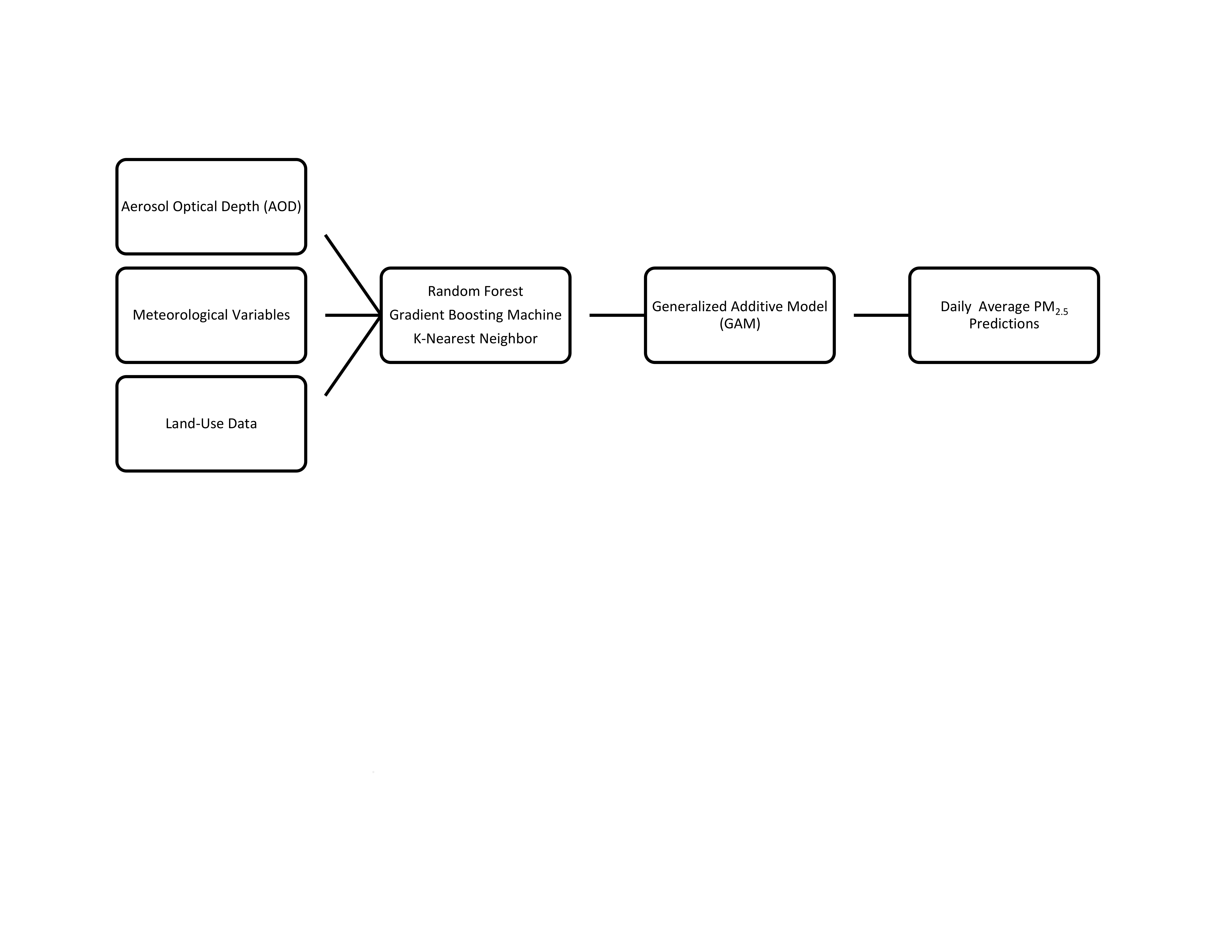
2. Materials and Methods
2.1. Machine Learning Algorithms
2.2. Input Variables
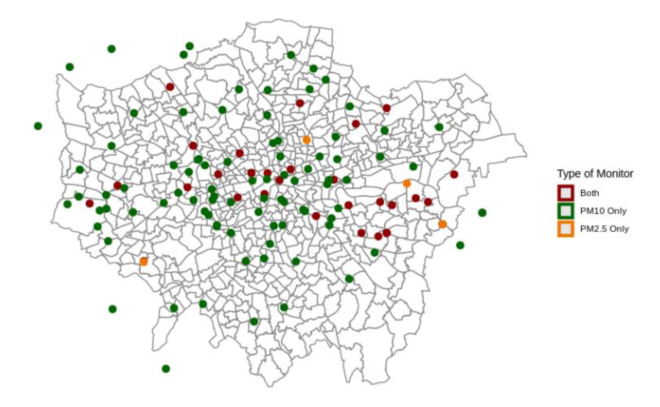
2.3. Data Sources
2.4. PM2.5 Data
2.5. Hyper-Parameter Tuning
2.6. Predictions
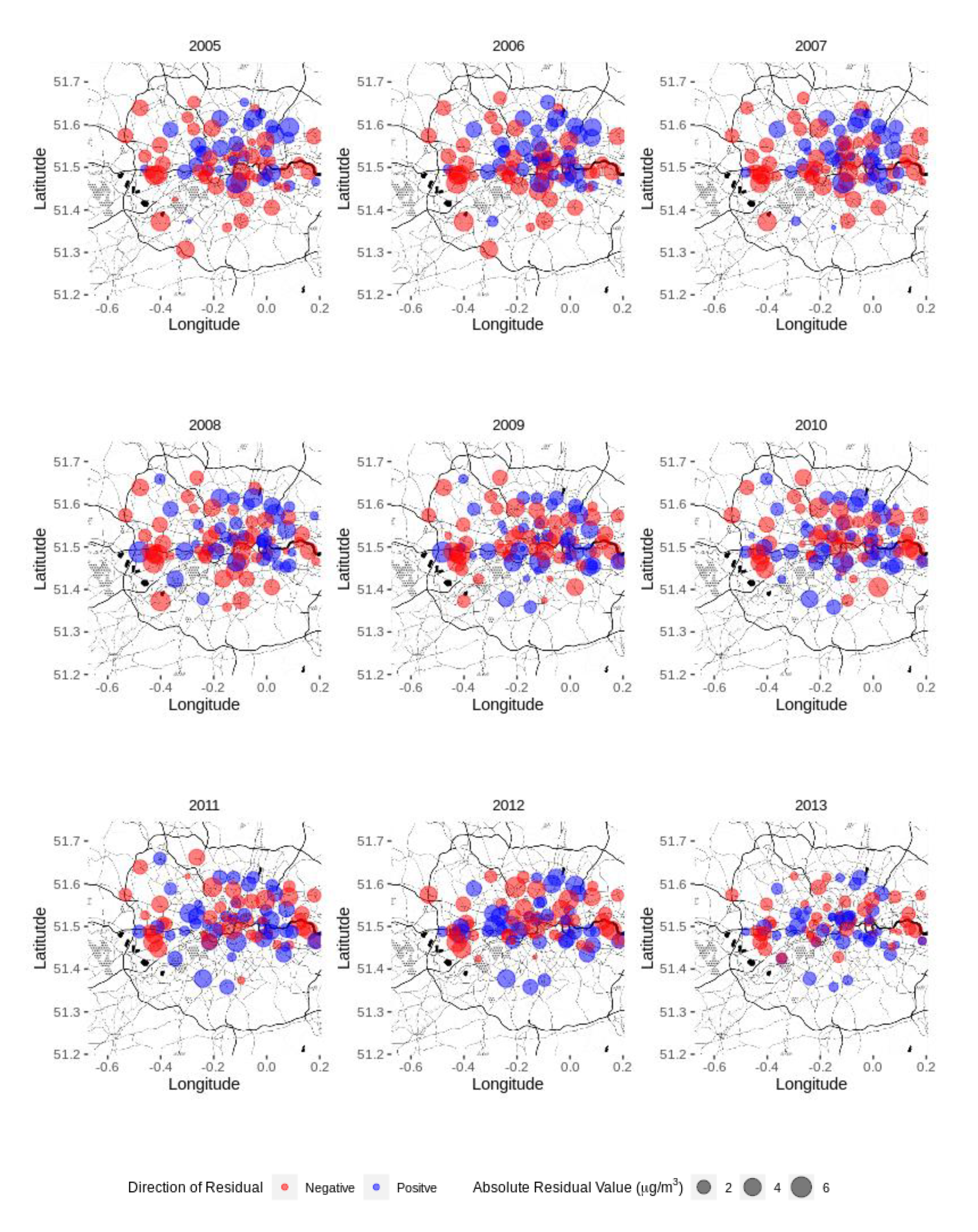
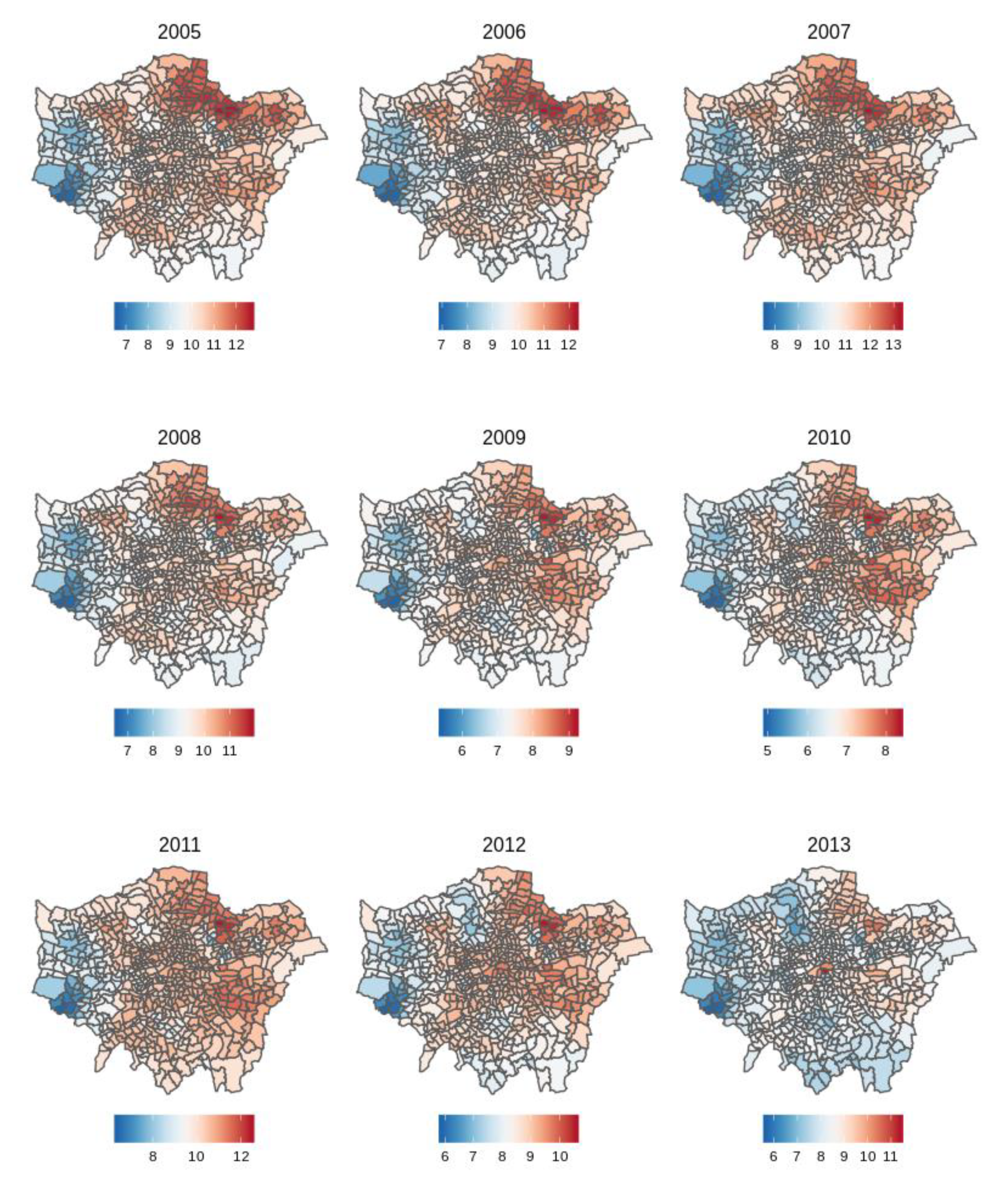
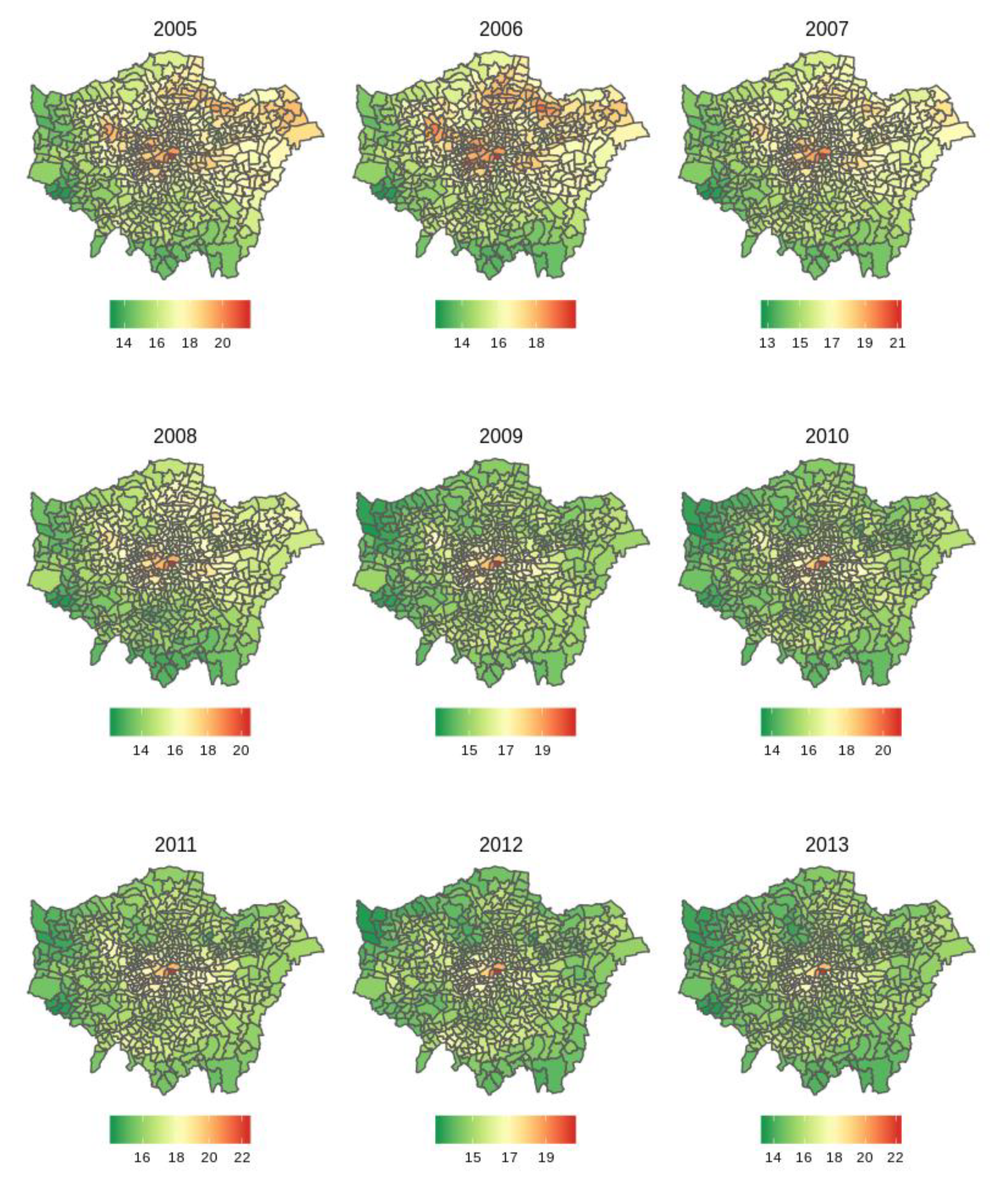
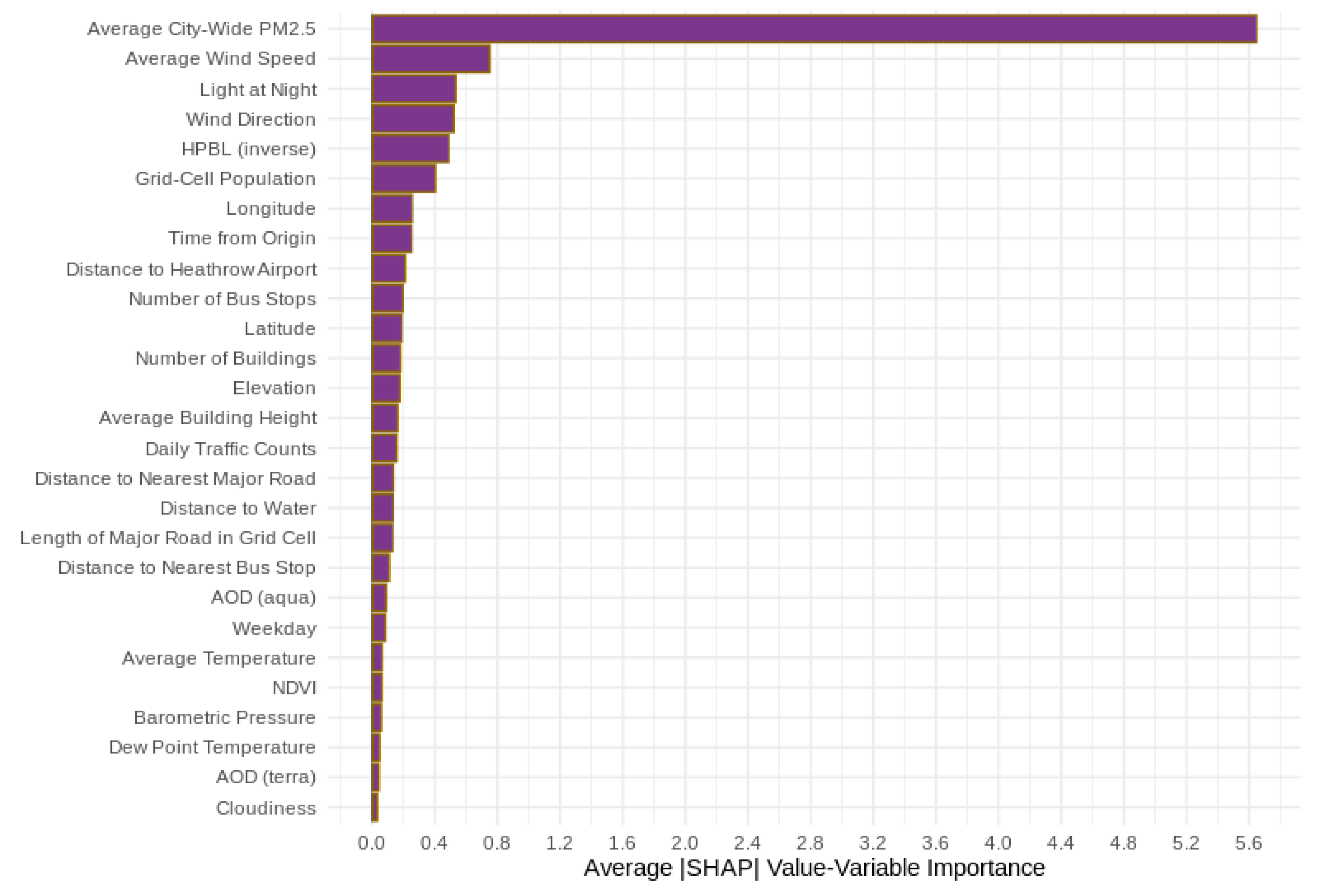
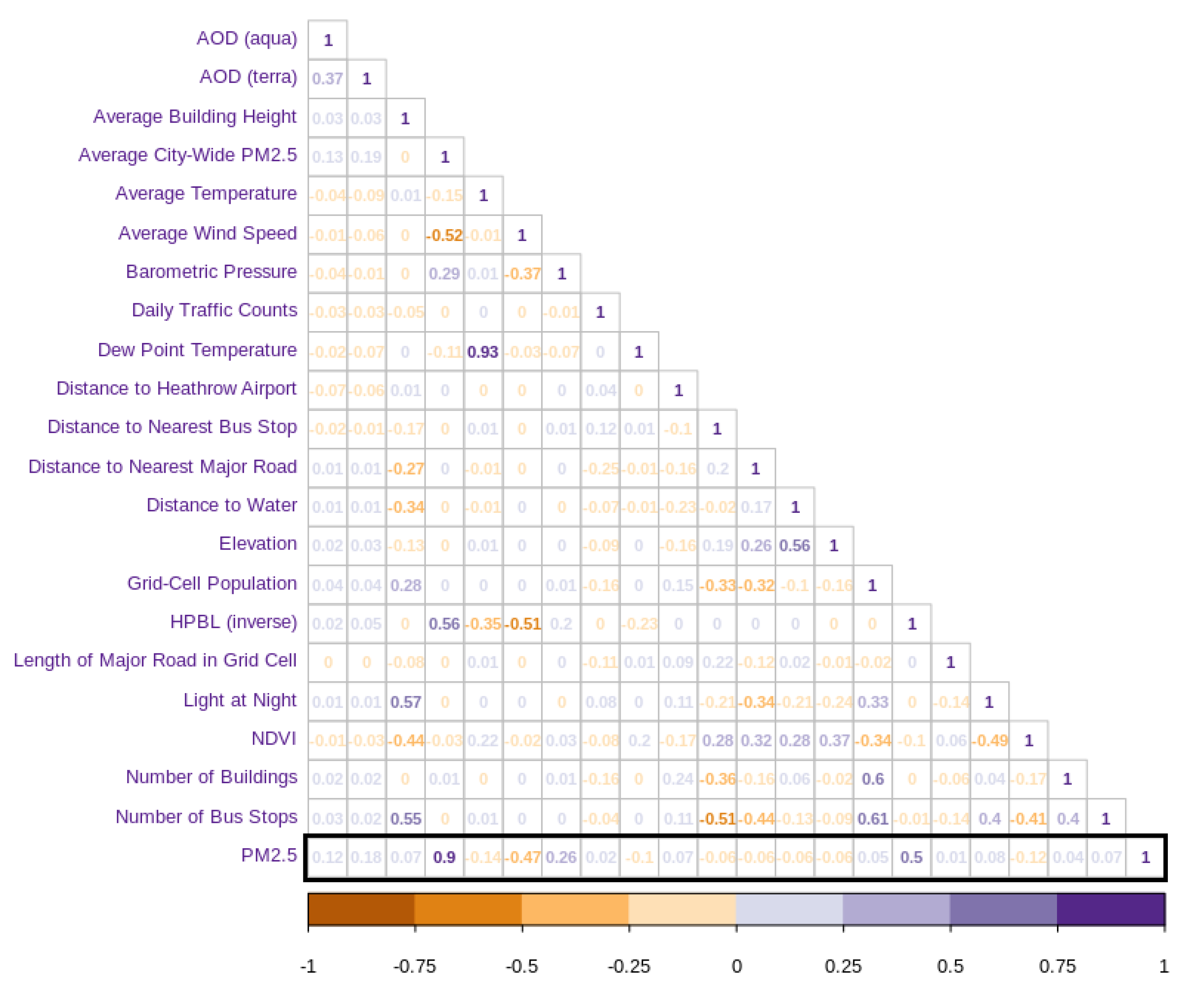
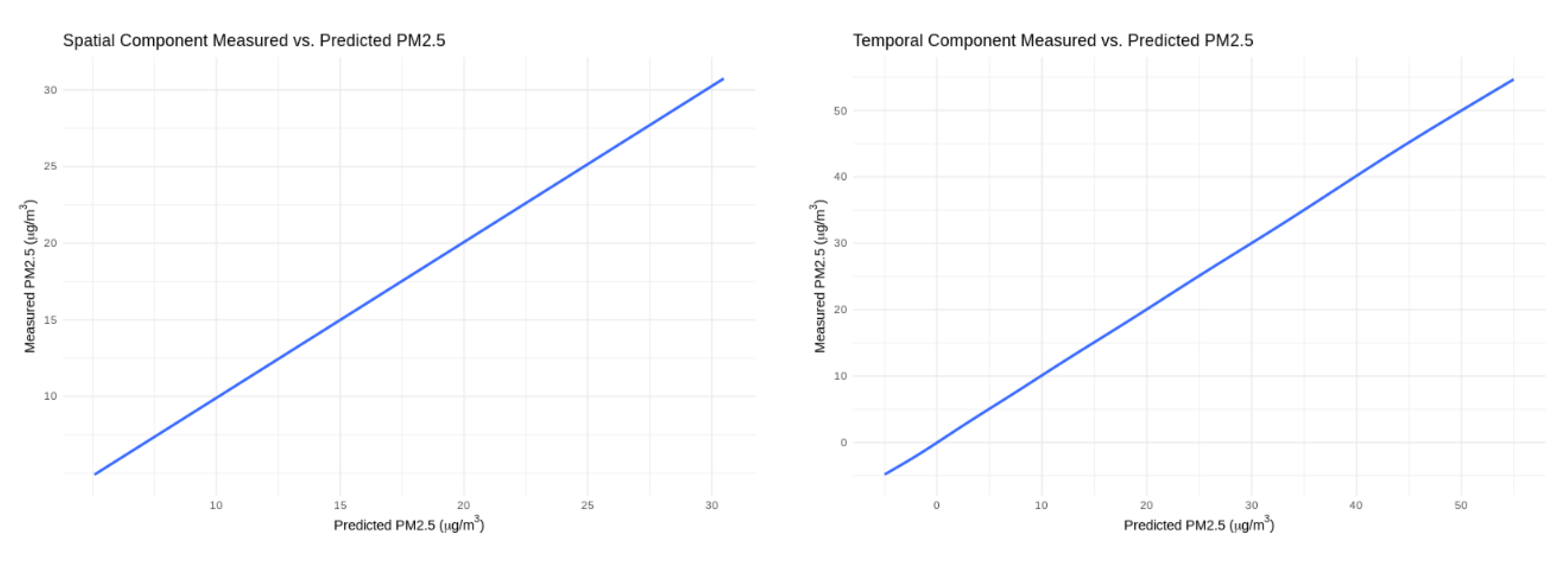
3. Results
4. Discussion
5. Conclusions
Author Contributions
Funding
Acknowledgments
Conflicts of Interest
References
- Sousan, S.; Koehler, K.; Hallett, L.; Peters, T.M. Evaluation of consumer monitors to measure particulate matter. J. Aerosol Sci. 2017, 107, 123–133. [Google Scholar] [CrossRef] [PubMed] [Green Version]
- Xing, Y.-F.; Xu, Y.-H.; Shi, M.-H.; Lian, Y.-X. The impact of PM2.5 on the human respiratory system. J. Thorac. Dis. 2016, 8, E69–E74. [Google Scholar] [PubMed]
- Dockery, D.W.; Pope, C.A.; Xu, X.; Spengler, J.D.; Ware, J.H.; Fay, M.E.; Ferris, B.G.; Speizer, F.E. An Association between Air Pollution and Mortality in Six U.S. Cities. N. Engl. J. Med. 1993, 329, 1753–1759. [Google Scholar] [CrossRef] [PubMed] [Green Version]
- Pope, C.A.; Thun, M.J.; Namboodiri, M.M.; Dockery, D.W.; Evans, J.S.; Speizer, F.E.; Heath, C.W.J. Particulate air pollution as a predictor of mortality in a prospective study of U.S. adults. Am. J. Respir. Crit. Care Med. 1995, 151, 669–674. [Google Scholar] [CrossRef]
- Wang, Y.; Shi, L.; Lee, M.; Liu, P.; Di, Q.; Zanobetti, A.; Schwartz, J.D. Long-term Exposure to PM2.5 and Mortality Among Older Adults in the Southeastern US. Epidemiology 2017, 28, 207–214. [Google Scholar] [CrossRef]
- Di, Q.; Wang, Y.; Zanobetti, A.; Wang, Y.; Koutrakis, P.; Choirat, C.; Dominici, F.; Schwartz, J.D. Air Pollution and Mortality in the Medicare Population. N. Engl. J. Med. 2017, 376, 2513–2522. [Google Scholar] [CrossRef]
- Vodonos, A.; Awad, Y.A.; Schwartz, J. The concentration-response between long-term PM2.5 exposure and mortality; A meta-regression approach. Environ. Res. 2018, 166, 677–689. [Google Scholar] [CrossRef]
- Atkinson, R.W.; Kang, S.; Anderson, H.R.; Mills, I.C.; Walton, H.A. Epidemiological time series studies of PM2.5 and daily mortality and hospital admissions: A systematic review and meta-analysis. Thorax 2014, 69, 660–665. [Google Scholar] [CrossRef] [Green Version]
- Amini, H.; Trang Nhung, N.T.; Schindler, C.; Yunesian, M.; Hosseini, V.; Shamsipour, M.; Hassanvand, M.S.; Mohammadi, Y.; Farzadfar, F.; Vicedo-Cabrera, A.M.; et al. Short-term associations between daily mortality and ambient particulate matter, nitrogen dioxide, and the air quality index in a Middle Eastern megacity. Environ. Pollut. 2019, 254, 113121. [Google Scholar] [CrossRef]
- Danesh Yazdi, M.; Wang, Y.; Di, Q.; Zanobetti, A.; Schwartz, J. Long-term exposure to PM2.5 and ozone and hospital admissions of Medicare participants in the Southeast USA. Environ. Int. 2019, 130, 104879. [Google Scholar] [CrossRef]
- Barnett, A.G.; Williams, G.M.; Schwartz, J.; Best, T.L.; Neller, A.H.; Petroeschevsky, A.L.; Simpson, R.W. The effects of air pollution on hospitalizations for cardiovascular disease in elderly people in Australian and New Zealand cities. Environ. Health Perspect. 2006, 114, 1018–1023. [Google Scholar] [CrossRef] [PubMed] [Green Version]
- Pun, V.C.; Kazemiparkouhi, F.; Manjourides, J.; Suh, H.H. Long-Term PM2.5 Exposure and Respiratory, Cancer, and Cardiovascular Mortality in Older US Adults. Am. J. Epidemiol. 2017, 186, 961–969. [Google Scholar] [CrossRef] [PubMed]
- Leiva, G.M.A.; Santibañez, D.A.; Ibarra, E.S.; Matus, C.P.; Seguel, R. A five-year study of particulate matter (PM2.5) and cerebrovascular diseases. Environ. Pollut. 2013, 181, 1–6. [Google Scholar] [CrossRef]
- Kioumourtzoglou, M.A.; Schwartz, J.D.; Weisskopf, M.G.; Melly, S.J.; Wang, Y.; Dominici, F.; Zanobetti, A. Long-term PM2.5 exposure and neurological hospital admissions in the northeastern United States. Environ. Health Perspect. 2016, 124, 23–29. [Google Scholar] [CrossRef] [Green Version]
- Fu, P.; Guo, X.; Cheung, F.M.H.; Yung, K.K.L. The association between PM2.5 exposure and neurological disorders: A systematic review and meta-analysis. Sci. Total Environ. 2019, 655, 1240–1248. [Google Scholar] [CrossRef]
- Shi, L.; Zanobetti, A.; Kloog, I.; Coull, B.A.; Koutrakis, P.; Melly, S.J.; Schwartz, J.D. Low-concentration PM2.5 and mortality: Estimating acute and chronic effects in a population-based study. Environ. Health Perspect. 2016, 124, 46–52. [Google Scholar] [CrossRef] [PubMed] [Green Version]
- Shaddick, G.; Thomas, M.L.; Amini, H.; Broday, D.; Cohen, A.; Frostad, J.; Green, A.; Gumy, S.; Liu, Y.; Martin, R.V.; et al. Data Integration for the Assessment of Population Exposure to Ambient Air Pollution for Global Burden of Disease Assessment. Environ. Sci. Technol. 2018, 52, 9069–9078. [Google Scholar] [CrossRef]
- Wang, J.; Christopher, S.A. Intercomparison between satellite-derived aerosol optical thickness and PM2.5 mass: Implications for air quality studies. Geophys. Res. Lett. 2003, 30, 2–5. [Google Scholar] [CrossRef]
- Liu, Y.; Park, R.J.; Jacob, D.J.; Li, Q.; Kilaru, V.; Sarnat, J.A. Mapping annual mean ground-level PM2.5 concentrations using Multiangle Imaging Spectroradiometer aerosol optical thickness over the contiguous United States. J. Geophys. Res. Atmos. 2004, 109, 1–10. [Google Scholar]
- Van Donkelaar, A.; Martin, R.V.; Park, R.J. Estimating ground-level PM2.5 using aerosol optical depth determined from satellite remote sensing. J. Geophys. Res. Atmos. 2006, 111, 1–10. [Google Scholar] [CrossRef]
- Van Donkelaar, A.; Martin, R.V.; Brauer, M.; Kahn, R.; Levy, R.; Verduzco, C.; Villeneuve, P.J. Global estimates of ambient fine particulate matter concentrations from satellite-based aerosol optical depth: Development and application. Environ. Health Perspect. 2010, 118, 847–855. [Google Scholar] [CrossRef] [PubMed] [Green Version]
- Gupta, P.; Christopher, S.A.; Wang, J.; Gehrig, R.; Lee, Y.; Kumar, N. Satellite remote sensing of particulate matter and air quality assessment over global cities. Atmos. Environ. 2006, 40, 5880–5892. [Google Scholar] [CrossRef]
- Kloog, I.; Koutrakis, P.; Coull, B.A.; Lee, H.J.; Schwartz, J. Assessing temporally and spatially resolved PM2.5 exposures for epidemiological studies using satellite aerosol optical depth measurements. Atmos. Environ. 2011, 45, 6267–6275. [Google Scholar] [CrossRef]
- Kloog, I.; Nordio, F.; Coull, B.A.; Schwartz, J. Incorporating local land use regression and satellite aerosol optical depth in a hybrid model of spatiotemporal PM2.5 exposures in the mid-atlantic states. Environ. Sci. Technol. 2012, 46, 11913–11921. [Google Scholar] [CrossRef] [Green Version]
- Moore, D.K.; Jerrett, M.; Mack, W.J.; Künzli, N. A land use regression model for predicting ambient fine particulate matter across Los Angeles, CA. J. Environ. Monit. 2007, 9, 246–252. [Google Scholar] [CrossRef]
- Smith, J.D.; Mitsakou, C.; Kitwiroon, N.; Barratt, B.M.; Walton, H.A.; Taylor, J.G.; Anderson, H.R.; Kelly, F.J.; Beevers, S.D. London Hybrid Exposure Model: Improving Human Exposure Estimates to NO2 and PM2.5 in an Urban Setting. Environ. Sci. Technol. 2016, 50, 11760–11768. [Google Scholar] [CrossRef] [Green Version]
- Geng, G.; Zhang, Q.; Martin, R.V.; van Donkelaar, A.; Huo, H.; Che, H.; Lin, J.; He, K. Estimating long-term PM2.5 concentrations in China using satellite-based aerosol optical depth and a chemical transport model. Remote Sens. Environ. 2015, 166, 262–270. [Google Scholar] [CrossRef]
- Di, Q.; Kloog, I.; Koutrakis, P.; Lyapustin, A.; Wang, Y.; Schwartz, J. Assessing PM2.5 Exposures with High Spatiotemporal Resolution across the Continental United States. Environ. Sci. Technol. 2016, 50, 4712–4721. [Google Scholar] [CrossRef] [Green Version]
- De Hoogh, K.; Gulliver, J.; van Donkelaar, A.; Martin, R.V.; Marshall, J.D.; Bechle, M.J.; Cesaroni, G.; Pradas, M.C.; Dedele, A.; Eeftens, M.; et al. Development of West-European PM2.5 and NO2 land use regression models incorporating satellite-derived and chemical transport modelling data. Environ. Res. 2016, 151, 1–10. [Google Scholar] [CrossRef] [Green Version]
- Taghavi-Shahri, S.M.; Fassò, A.; Mahaki, B.; Amini, H. Concurrent spatiotemporal daily land use regression modeling and missing data imputation of fine particulate matter using distributed space-time Expectation Maximization. Atmos. Environ. 2019, 117202. [Google Scholar] [CrossRef]
- Di, Q.; Amini, H.; Shi, L.; Kloog, I.; Silvern, R.; Kelly, J.; Sabath, M.B.; Choirat, C.; Koutrakis, P.; Lyapustin, A.; et al. An ensemble-based model of PM2.5 concentration across the contiguous United States with high spatiotemporal resolution. Environ. Int. 2019, 130, 104909. [Google Scholar] [CrossRef] [PubMed]
- Di, Q.; Rowland, S.; Koutrakis, P.; Schwartz, J. A hybrid model for spatially and temporally resolved ozone exposures in the continental United States A hybrid model for spatially and temporally resolved ozone exposures in the continental A hybrid model. J. Air Waste Manag. Assoc. 2017, 67, 39–52. [Google Scholar] [CrossRef] [PubMed] [Green Version]
- Lary, D.J.; Lary, T.; Sattler, B. Using Machine Learning to Estimate Global PM2.5 for Environmental Health Studies. Environ. Health Insights 2015, 9, 41–52. [Google Scholar] [CrossRef] [PubMed]
- Weizhen, H.; Zhengqiang, L.; Yuhuan, Z.; Hua, X.; Ying, Z.; Kaitao, L.; Donghui, L.; Peng, W.; Yan, M. Using support vector regression to predict PM10 and PM2.5. IOP Conf. Ser. Earth Environ. Sci. 2014, 17, 012268. [Google Scholar] [CrossRef] [Green Version]
- Wei, J.; Huang, W.; Li, Z.; Xue, W.; Peng, Y.; Sun, L.; Cribb, M. Estimating 1-km-resolution PM2.5 concentrations across China using the space-time random forest approach. Remote Sens. Environ. 2019, 231, 111221. [Google Scholar] [CrossRef]
- Di, Q.; Amini, H.; Shi, L.; Kloog, I.; Silvern, R.F.; Kelly, J.T.; Sabath, M.B.; Choirat, C.; Koutrakis, P.; Lyapustin, A.; et al. Assessing NO2 Concentration and Model Uncertainty with High Spatiotemporal Resolution across the Contiguous United States Using Ensemble Model Averaging. Environ. Sci. Technol. 2020, 54, 1372–1384. [Google Scholar] [CrossRef]
- Wang, Y.; Lee, M.; Liu, P.; Shi, L.; Yu, Z.; Awad, Y.A.; Zanobetti, A.; Schwartz, J.D. Doubly Robust Additive Hazards Models to Estimate Effects of a Continuous Exposure on Survival. Epidemiology 2017, 28, 771–779. [Google Scholar] [CrossRef]
- Chen, G.; Jin, Z.; Li, S.; Jin, X.; Tong, S.; Liu, S.; Yang, Y.; Huang, H.; Guo, Y. Early life exposure to particulate matter air pollution (PM1, PM2.5 and PM10) and autism in Shanghai, China: A case-control study. Environ. Int. 2018, 121, 1121–1127. [Google Scholar] [CrossRef]
- Qiu, X.; Wei, Y.; Wang, Y.; Di, Q.; Sofer, T.; Awad, Y.A.; Schwartz, J. Inverse probability weighted distributed lag effects of short-term exposure to PM2.5 and ozone on CVD hospitalizations in New England Medicare participants—Exploring the causal effects. Environ. Res. 2020, 182, 109095. [Google Scholar] [CrossRef]
- Van Der Laan, M.J.; Polley, E.C.; Hubbard, A.E. Super learner. Stat. Appl. Genet. Mol. Biol. 2007, 6. [Google Scholar] [CrossRef]
- Friedman, J.H. Greedy function approximation: A gradient boosting machine. Ann. Stat. 2001, 29, 1189–1232. [Google Scholar] [CrossRef]
- Breiman, L. Random forests. Mach. Learn. 2001, 45, 5–32. [Google Scholar] [CrossRef] [Green Version]
- Glorot, X.; Bordes, A.; Bengio, Y. Deep Sparse Rectifier Neural Networks. In Proceedings of the Fourteenth International Conference on Artificial Intelligence and Statistics, Ft. Lauderdale, FL, USA, 11–13 April 2011; pp. 315–323. [Google Scholar]
- Altman, N.S. An Introduction to Kernel and Nearest-Neighbor Nonparametric Regression. Am. Stat. 1992, 46, 175–185. [Google Scholar]
- Lyapustin, A.; Wang, Y.; Korkin, S.; Huang, D. MODIS Collection 6 MAIAC algorithm. Atmos. Meas. Tech. 2018, 11, 5741–5765. [Google Scholar] [CrossRef] [Green Version]
- Center for International Earth Science Information Network—CIESIN—Columbia University Gridded Population of the World, Version 4 (GPWv4): Population Density, Revision 11; NASA Socioeconomic Data and Applications Center (SEDAC): Palisades, NY, USA, 2018. [CrossRef]
- Environmental Research Groupt at King’s College London London Air. Available online: http://londonair.org.uk/LondonAir/Default.aspx (accessed on 15 December 2019).
- Department of Environment Food & Rural Affairs UK Automatic Urban and Rural Network. Available online: https://uk-air.defra.gov.uk/ (accessed on 15 December 2019).
- Analitis, A.; Barratt, B.M.; Green, D.; Beddows, A.; Samoli, E.; Schwartz, J.D.; Katsouyanni, K. Enhancement of the PM2.5 Database 2004–2013 for London within the STEAM Project Using Generalized Additive Models and Machine Learning Methods. Unpublished work. 2020; 1–20. [Google Scholar]
- LeDell, E.; Gill, N.; Aiello, S.; Fu, A.; Candel, A.; Click, C.; Kraljevic, T.; Nykodym, T.; Aboyoun, P.; Kurka, M.; et al. h2o: R Interface for “H2O”. Available online: https://github.com/h2oai/h2o-3 (accessed on 1 March 2020).
- Kuhn, M. Building predictive models in R using the caret package. J. Stat. Softw. 2008, 28, 1–26. [Google Scholar] [CrossRef] [Green Version]
- Lundberg, S.M.; Lee, S.I. A unified approach to interpreting model predictions. Adv. Neural Inf. Process. Syst. 2017, 2017, 4766–4775. [Google Scholar]
- Samoli, E.; Butland, B.; Rodopoulou, S.; Atkinson, R.W.; Barratt, B.M.; Beevers, S.D.; Dimakopoulou, K.; Danesh Yazdi, M.; Schwartz, J.D.; Katsouyanni, K. The Impact of Measurement Error in Modelled Ambient Particles Exposures on Health Effect Estimates in Multi-level Analysis: A Simulation Study. Unpublished work. 2020. [Google Scholar]
- Singh, V.; Sokhi, R.S.; Kukkonen, J. PM2.5 concentrations in London for 2008-A modeling analysis of contributions from road traffic. J. Air Waste Manag. Assoc. 2014, 64, 509–518. [Google Scholar] [CrossRef] [Green Version]
- Eeftens, M.; Beelen, R.; De Hoogh, K.; Bellander, T.; Cesaroni, G.; Cirach, M.; Declercq, C.; Dedele, A.; Dons, E.; De Nazelle, A.; et al. Development of land use regression models for PM2.5, PM2.5 absorbance, PM10 and PMcoarse in 20 European study areas; Results of the ESCAPE project. Environ. Sci. Technol. 2012, 46, 11195–11205. [Google Scholar] [CrossRef]
- Xiao, Q.; Chang, H.H.; Geng, G.; Liu, Y. An Ensemble Machine-Learning Model to Predict Historical PM2.5 Concentrations in China from Satellite Data. Environ. Sci. Technol. 2018, 52, 13260–13269. [Google Scholar] [CrossRef] [PubMed]
- Zhan, Y.; Luo, Y.; Deng, X.; Chen, H.; Grieneisen, M.L.; Shen, X.; Zhu, L.; Zhang, M. Spatiotemporal prediction of continuous daily PM2.5 concentrations across China using a spatially explicit machine learning algorithm. Atmos. Environ. 2017, 155, 129–139. [Google Scholar] [CrossRef]
- Chen, G.; Li, S.; Knibbs, L.D.; Hamm, N.A.S.; Cao, W.; Li, T.; Guo, J.; Ren, H.; Abramson, M.J.; Guo, Y. A machine learning method to estimate PM2.5 concentrations across China with remote sensing, meteorological and land use information. Sci. Total Environ. 2018, 636, 52–60. [Google Scholar] [CrossRef] [PubMed]
- Xu, Y.; Ho, H.C.; Wong, M.S.; Deng, C.; Shi, Y.; Chan, T.C.; Knudby, A. Evaluation of machine learning techniques with multiple remote sensing datasets in estimating monthly concentrations of ground-level PM2.5. Environ. Pollut. 2018, 242, 1417–1426. [Google Scholar] [CrossRef]
- Huang, C.J.; Kuo, P.H. A deep cnn-lstm model for particulate matter (PM2.5) forecasting in smart cities. Sensors 2018, 18, 2220. [Google Scholar] [CrossRef] [PubMed] [Green Version]
- Just, A.C.; De Carli, M.M.; Shtein, A.; Dorman, M.; Lyapustin, A.; Kloog, I. Correcting measurement error in satellite aerosol optical depth with machine learning for modeling PM2.5 in the Northeastern USA. Remote Sens. 2018, 10, 803. [Google Scholar] [CrossRef] [Green Version]
- Li, J.; Carlson, B.E.; Lacis, A.A. How well do satellite AOD observations represent the spatial and temporal variability of PM2.5 concentration for the United States? Atmos. Environ. 2015, 102, 260–273. [Google Scholar] [CrossRef]


| Model | Overall R2 | RMSE | Intercept | Slope | Spatial R2 | RMSE | Intercept | Slope | Temporal R2 | RMSE | Intercept | Slope |
|---|---|---|---|---|---|---|---|---|---|---|---|---|
| RF | 0.830 | 4.278 | −0.120 | 0.989 | 0.386 | 2.660 | −0.827 | 1.032 | 0.886 | 3.297 | 0.000 | 0.988 |
| GBM | 0.826 | 4.331 | 0.081 | 0.978 | 0.393 | 2.644 | −0.328 | 1.003 | 0.880 | 3.381 | 0.000 | 0.978 |
| NN | 0.793 | 4.728 | 0.179 | 0.956 | 0.266 | 3.033 | 4.92 | 0.671 | 0.861 | 3.642 | 0.000 | 0.976 |
| KNN | 0.791 | 4.721 | 0.107 | 0.965 | 0.237 | 2.985 | 2.356 | 0.826 | 0.863 | 3.623 | 0.000 | 0.972 |
| Final Ensemble Model | 0.828 | 4.231 | 0.058 | 0.979 | 0.396 | 2.637 | −0.216 | 0.996 | 0.882 | 3.556 | 0.000 | 0.979 |
| Year | Moran’s I | p-Value |
|---|---|---|
| 2005 | −0.0132 | 0.446 |
| 2006 | −0.0123 | 0.603 |
| 2007 | −0.0125 | 0.953 |
| 2008 | −0.0118 | 0.848 |
| 2009 | −0.0114 | 0.552 |
| 2010 | −0.0119 | 0.380 |
| 2011 | −0.0116 | 0.167 |
| 2012 | −0.0118 | 0.338 |
| 2013 | −0.0122 | 0.500 |
| Minimum | 25th Percentile | Median | Mean | 75th Percentile | Maximum | Standard Deviation | |
|---|---|---|---|---|---|---|---|
| Daily Measured PM2.5 | 2.9 | 10.0 | 13.1 | 16.0 | 19.0 | 77.5 | 9.2 |
| Daily Predicted PM2.5 (Monitoring Sites) | 2.9 | 10.0 | 13.2 | 16.0 | 19.0 | 77.4 | 9.2 |
| Daily Predicted PM2.5 (Grid-cells) | 2.8 | 9.0 | 12.2 | 14.9 | 17.9 | 74.4 | 9.0 |
| Annual Measured PM2.5 | 15.3 | 15.6 | 16.1 | 16.1 | 16.2 | 17.1 | 0.6 |
| Annual Predicted PM2.5 (Monitoring Sites) | 15.3 | 15.6 | 16.1 | 16.1 | 16.2 | 17.0 | 0.6 |
| Annual Predicted PM2.5 (Grid-cells) | 14.1 | 14.5 | 14.7 | 14.9 | 15.2 | 15.9 | 0.6 |
| Random Forest | Gradient Boosting Machine | ||
|---|---|---|---|
| Variable | Relative Contribution (%) | Variable | Relative Contribution (%) |
| Average city-wide daily PM2.5 | 58.31 | Average city-wide daily PM2.5 | 66.75 |
| Height of the planetary boundary layer (inverse) | 10.28 | Average wind speed | 6.36 |
| Average wind speed | 6.90 | Wind direction (categorical) | 5.00 |
| Wind direction (categorical) | 4.65 | Height of the planetary boundary layer (inverse) | 2.69 |
| AOD (from aqua satellite) | 1.17 | Time (days from January 1, 2005) | 1.26 |
| Average barometric pressure | 1.10 | Distance to Heathrow airport | 1.22 |
| Distance to Heathrow airport | 0.99 | Population density | 1.10 |
| Longitude | 0.96 | Light at night | 1.05 |
| Light at night | 0.94 | Average building height in grid cell | 1.00 |
| Average temperature | 0.93 | Number of buildings in grid cell | 0.98 |
© 2020 by the authors. Licensee MDPI, Basel, Switzerland. This article is an open access article distributed under the terms and conditions of the Creative Commons Attribution (CC BY) license (http://creativecommons.org/licenses/by/4.0/).
Share and Cite
Danesh Yazdi, M.; Kuang, Z.; Dimakopoulou, K.; Barratt, B.; Suel, E.; Amini, H.; Lyapustin, A.; Katsouyanni, K.; Schwartz, J. Predicting Fine Particulate Matter (PM2.5) in the Greater London Area: An Ensemble Approach using Machine Learning Methods. Remote Sens. 2020, 12, 914. https://doi.org/10.3390/rs12060914
Danesh Yazdi M, Kuang Z, Dimakopoulou K, Barratt B, Suel E, Amini H, Lyapustin A, Katsouyanni K, Schwartz J. Predicting Fine Particulate Matter (PM2.5) in the Greater London Area: An Ensemble Approach using Machine Learning Methods. Remote Sensing. 2020; 12(6):914. https://doi.org/10.3390/rs12060914
Chicago/Turabian StyleDanesh Yazdi, Mahdieh, Zheng Kuang, Konstantina Dimakopoulou, Benjamin Barratt, Esra Suel, Heresh Amini, Alexei Lyapustin, Klea Katsouyanni, and Joel Schwartz. 2020. "Predicting Fine Particulate Matter (PM2.5) in the Greater London Area: An Ensemble Approach using Machine Learning Methods" Remote Sensing 12, no. 6: 914. https://doi.org/10.3390/rs12060914