Retrieval of Garstang's emission function from all-sky camera images

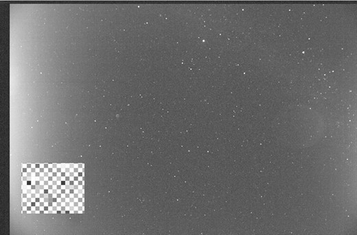
Typical RAW picture of a sky including the border with shielded pixels. Inset: detailed view to the individual pixel values. The contrast and the brightness of the picture were adjusted artificially to show clearly all important parts of the sky.

There is a specific problem when DSLRs are used in night light measurements; occasionally it is impossible to capture a picture not containing extremely bright objects (mainly lighting fixtures that shines directly on the lens producing an image on the sensor). Such small but extremely bright areas can significantly shift the resulting values of calculated integrals. Therefore, these small very bright areas were replaced by a median value of the picture brightness. However, this procedure was applied only to a few pictures, while the majority of disturbed sky scans were rather ignored.

The whole data pre-processing algorithm for both cameras (60d and D80) is the following.

Conversion of CR2 (Canon/Nikon RAW) to 16-bit PGM file using dcraw.
Calculation of mean zero-level from covered pixels (left-hand and upper border in Fig. 1).
Subtraction of zero-level from individual pixel values.
The small extremely bright objects were replaced by the median of the picture brightness if e.g. some pixel values are five or more times higher than that for the rest of the sky.
Retrieval of brightness in red, green and blue part of the spectrum using the information on type and position of the colour mask.
Such pre-processed picture was used for later calculations.

2.3 Lens calibration

Although the DSLR camera is suitable for lighting analysis its use for skyglow measurement has been limited by the lack of a correct calibration procedure. For instance, there are certain drawbacks associated with the use of non-calibrated lens.

The function f(θ, ϕ, x, y) that represents a projection of sky vault onto the sensor must be known to find the corresponding pixel coordinates x, y for a sky element with zenith θ and azimuth ϕ angles.
The transformation of sky radiance into the electric signal at the sensor depends on θ and can be expressed through so-called sensitivity function g(θ).

The functions f(θ, ϕ, x, y) and g(θ) were determined in laboratory conditions using a calibration technique that provides information on both (i) the symmetric distortion of fisheye lenses, and (ii) the correction of the x, y pixel coordinates. Tests of the system were performed in dark room with the purpose to find the lenses distortion and the projection angle. Having a calibration target fixed several pictures were taken at different exposure times and angles. Specifically, a small light source based on white led was placed 1 m away from the objective lens on its optical axis. Afterwards, the camera was moved relatively to the axis of the light source to obtain various values of θ. In each position a picture of the light source was captured. Using a standard picture processing software (e.g. adobe photoshop or corel photopaint) the position of the centre of the light source on the sensor was found and its brightness has been determined. Assuming an axial symmetry of the lens, the functions f(θ, ϕ, x, y) and g(θ) were constructed over θ, where the upper projection limit for the angle θ depends on the lens (see Figs 4 and 5).

Using above-mentioned data the position x, y of a pixel on the sensor corresponding to θ, ϕ can be obtained as follows:

\begin{eqnarray} x &=& x_0 + r\cos \phi , \nonumber\\ y &=& y_0 + r\sin \phi , \nonumber\\ r &=& f\left( \theta \right), \end{eqnarray}

(1)

where x₀, y₀ is the position of the centre pixel (light source is placed on the axis of the lens), implying the position of any pixel can be drawn as a function of θ (see Figs 2 and 4). Correspondingly, the sensitivity function g(θ, ϕ) = g(θ) is plotted in Figs 3 and 5.

Figure 2.

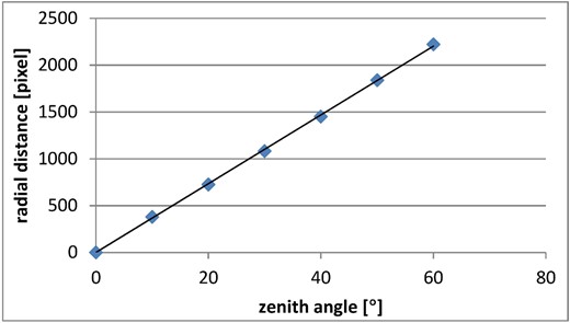
Pixel radial distance as a function of observational zenith angle θ for Canon 60d with incomplete hemispherical projection. The image is a rectangle (167° × 120°) producing a 180° FOV on the diagonal, but limiting the maximum of projected zenith distance to 60 on the short side.

Figure 3.

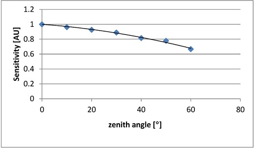
Relative sensitivity for Canon 60d embedded sensor as a function of zenith angle.

Figure 4.

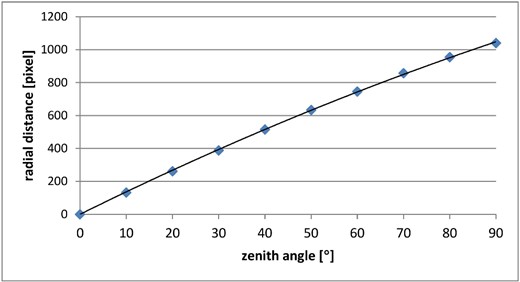
Nikon projection function plotted as pixel radial distance versus observational zenith angle θ.

Figure 5.

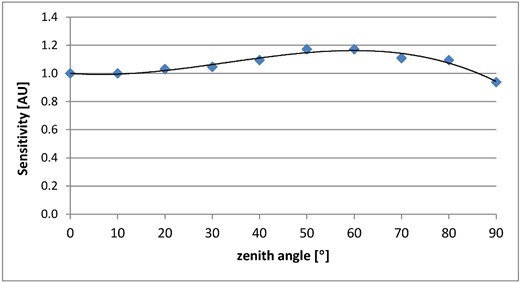
Relative sensitivity for Nikon embedded sensor as a function of zenith angle.

2.4 Data processing

The data recorded from the whole hemisphere were used to calculate horizontally projected irradiance, while a small circular area at zenith was taken into account when determining the zenith brightness. Any requested area of the picture was divided into small parts of size Δθ, Δϕ. The amount of such parts predetermines the precision of the calculation, but also a computational time. In our model we have used a grid of size 5000 × 5000 that has been equally applied to irradiance and radiance calculations.

2.4.1 Zenith brightness calculation

Using the calibration functions mentioned above we have calculated the zenith brightness as follows:

\begin{equation} B\left( \theta \right) = \frac{{\mathop \sum \nolimits_i \sum\nolimits_j {\frac{{I\left( {\theta _i ,\phi _j } \right)}}{{g\left( {\theta _i } \right)}}} \sin \theta _i \Delta \theta _i \Delta \phi _j }}{{\mathop \sum \nolimits_i \sum\nolimits_j {\sin \theta _i \Delta \theta _i \Delta \phi _j } }}, \end{equation}

(2)

where data reading from a scanned image runs over circular rings centred in the zenith with zenith distances θ_i = 0…θ. Here I(θ_i, ϕ_j) is the pixel value of the nearest (red, green or blue) pixel corresponding to a given sky position (θ, ϕ). The value of θ should be as small as possible, but large enough for having a good statistics of pixels to get a stable average over I(θ_i, ϕ_j).

2.4.2 Horizontal surface irradiance calculation

Using the same data grid, the horizontal irradiance is obtained as

\begin{equation} D = \sum\limits_i {\sum\limits_j {\frac{{I\left( {\theta _i ,\phi _j } \right)}}{{g\left( {\theta _i } \right)}}} } \;\sin \theta _i \cos \theta _i \Delta \theta _i \Delta \phi _j . \end{equation}

(3)

In both cases (in equation 2 or equation 3), the intensity I(θ_i, ϕ_j) was determined from I(x_i, y_j) by applying a backward transformation, i.e. mapping the polar coordinates to Cartesian coordinates. The software solution we have developed is fully automatized and runs over all pictures in database, while each fisheye image contains information on both zenith brightness and horizontal irradiance. It is important to mention that horizontal irradiance was only obtained for Nikon images, while it was necessary to cut the picture in a circular pattern (50º from the centre) in order to obtain the incomplete horizontal irradiance for Canon images. It is because acceptance angle for lens used on the Canon camera makes a readout of low beams impossible. Subsequently, the radiance data were obtained from the same picture cutting a small circle in the zenith of the circumference. Then, the ratio B(θ)/D was obtained at different distances from a city.

3 THEORETICAL METHODS

It has been shown by Kocifaj & Solano Lamphar (2014) that parameters of Garstang's emission function can be obtained from ratios of zenith radiance to horizontal irradiance, both measured at set of discrete distances from a city. Nevertheless, the solution concept is easily applicable to any type of emission function that has an analytical form and is parametrized through the total uplight (F) and the fraction of reflected light (G).

Retrieval technique requires that the N-dimensional vector |${\boldsymbol r}_{\rm T}$| with elements |$\left[ {B\left( \theta \right)/D} \right]_i^{\rm T}$|(i ∈ 〈1, N〉) is computed at N discrete distances from a city and consequently |${\boldsymbol r}_{\rm T}$| is compared against |${\boldsymbol r}_{\rm E}$| that is equally sized vector containing the ratios of |$\left[ {B\left( \theta \right)/D} \right]_i^{\rm E}$| experimentally determined at the same set of distances. The parameters F and G are found by minimizing the quadratic form of differences between theoretically predicted and measured data, i.e. |$\left| {{\boldsymbol r}_{\rm T} - {\boldsymbol r}_{\rm E} } \right|_{F,G}^2$|⁠. The simplest way how to do this is to use the least-square method, but in more general case the solution S_{F, G} is sought by minimizing the functional |$\left| {{\bf K}_{\bf T} S_{F,G} - {\boldsymbol r}_{\rm E} - {\boldsymbol \varepsilon }} \right|_{}^2$|⁠, where |${\bf K}_{\bf T}$| is an integral operator acting on solution function S_{F, G} so that |${\bf K}_{\bf T} S_{F,G} = {\boldsymbol r}_{\rm T}$| and |${\boldsymbol \varepsilon }$| is noise vector that represents experimental errors in each measuring point. The system of equations to be solved is most typically overdetermined since the measurements are made at more than 2–3 distances. It is therefore not a difficult task to find the best fit to F and G, although the minimum error that has been achieved can be still large enough. Besides experimental errors, such a weak convergence can either indicate optical instability of the atmosphere during a field campaign, or inconvenience of the theoretical model. However, such information is also valuable, since it suggests that the emission function of a city is most probably different from that considered by Garstang. This finding is a challenge for modellers who are encouraged to search for more appropriate model of radiant intensity distributions, but also for experimentalists who can gather as much data as possible near isolated cities under optically stable atmospheric conditions with aim to build worldwide database of data vectors |${\boldsymbol r}_{\rm E}$|⁠. Systematic processing of best data sets can finally provide proper information about F and G or can be used to verify the range of applicability of different emission functions including that of Garstang-like.

The theoretical ratio of B(θ)/D typically changes quickly in city surroundings and alter with F or G as shown in figs 2 and 4 in the paper by Kocifaj & Solano Lamphar (2014). It is therefore convenient to get a good data base of B(θ)/D for distances of few city radii from the city edge. In practically important cases G is usually a known value, as it characterizes the underlying surface. For instance, ground albedo of a soil surfaces can be as large as 0.4 or even more, while the fraction of light reflected by a vegetation is often below 0.1 in blue and yellow parts of the spectrum. But, some plants can reflect about 20 per cent of an incident light at wavelengths above 600 nm (Mishev 1985). Reflectance mapping is possible from satellite imagery, and also from ground-based measurements under overcast conditions (see e.g. Shiffrin & Kozhaev 1972). In contrast, F involves a bulk effect of all light sources (streets, advertisement boards, building interiors, etc.), each having different spectral emissivity and directionality, and each being situated in different environment. It is difficult or rather impossible to compute F taking all of these sources into consideration accepting their complex distributions in an urban territory. For this reason F is an unknown quantity that needs to be determined by indirect methods. Based on the theoretical model by Kocifaj & Solano Lamphar (2014), F can also be inferred from Sky Quality Meter (SQM) data. SQM is a portable device that measures zenith radiance in small acceptance angle. Assuming that G is available for a given locality, the uplight can be obtained from the following equation:

\begin{equation} F = \frac{{\rho \left( {G,V,d_1 ,d_2 ,\frac{{B_{d1} }}{{B_{d2} }}} \right)}}{{\zeta \left( {V,d_1 ,d_2 ,\frac{{B_{d1} }}{{B_{d2} }}} \right) + \rho \left( {G,V,d_1 ,d_2 ,\frac{{B_{d1} }}{{B_{d2} }}} \right)}}, \end{equation}

(4)

where

\begin{eqnarray} \rho \left( {G,V,d_1 ,d_2 ,\frac{{B_{d1} }}{{B_{d2} }}} \right) &=& 2G\Bigg\{ \exp \left[ { - \frac{K}{V}\left( {d_1 - d_2 } \right)} \right]\nonumber\\ &&\times R_{\cos } \left( {\frac{{Kd_1 }}{V}} \right) - \frac{{B_{d1} }}{{B_{d2} }}R_{\cos } \left( {\frac{{Kd_2 }}{V}} \right) \Bigg\}\nonumber\\ \end{eqnarray}

(5)

and

\begin{eqnarray} \zeta \left( {V,d_1 ,d_2 ,\frac{{B_{d1} }} {{B_{d2} }}} \right) &=& 0.554\quad \Bigg\{ \frac{{B_{d1} }}{{B_{d2} }}\quad R_4 \left( {\frac{{K\;d_2 }}{V}} \right)\nonumber\\ &&- \exp \left[ { - \frac{K}{V}\left( {d_1 - d_2 } \right)} \right]\quad R_4 \left( {\frac{{K\;d_1 }}{V}} \right) \Bigg\}.\nonumber\\ \end{eqnarray}

(6)

Here, K = 3.912 is the so-called Koschmieder constant, which characterizes the standard visibility or visual range V (Middleton 1968) under the assumption that the contrast threshold for an observed target is 0.02 (Horvath 1995), while the functions R₄ and R_cos can be found in Kocifaj & Solano Lamphar (2014). Note that the horizontal visibility (V) is commonly measured at actinometric or meteorological stations, and, the ratio of K/V is consequently used to determine the horizontal extinction coefficient (km⁻¹). B_d1 and B_d2 are zenith radiances measured at distances d₁ and d₂ from the city centre, respectively. The measurements made at a number of distances form an overdetermined system that can benefit from higher accuracy of F. In addition, no calibration of experimentally determined radiances is necessary since we evaluate the ratio of two values recorded using the same device rather than two absolute values obtained independently of each other. However, the correction of SQM data has to be made under varying temperature conditions as suggested by Schnitt et al. (2013).

4 INFORMATION CONTENT OF EXPERIMENTAL DATA

The height of the light fixtures might appear a limiting factor in numerical inversion of the optical data near the city edges. The street lighting luminaire are usually situated several metres above the ground, thus tends to illuminate a measuring device by direct. The situation is even worse with tall buildings that emit the light toward all directions and can influence the measured data at several hundred metres from the light source. Fortunately, the data vector |${\boldsymbol r}_{\rm E}$| can be also constructed from incompatible set of |$\left[ {B\left( \theta \right)/D} \right]_i^{\rm E}$|⁠, where D can be either complete or incomplete horizontally projected irradiance. In reality it means that different masking of horizon can be applied to limit the instrument FOV. The only requirement is that all data must be gathered by the same device (i.e. by the same camera). Once the nature of data vector elements is known, the corresponding theoretical values of |${\boldsymbol r}_{\rm T}$| can be computed. The minimization runs as described earlier in Section 3. It might appear desirable to reduce FOV near the city edges, since we can avoid unnecessary peaks due to direct light from some luminaires, but also unnecessary intensity decay due to high-elevation masking.

The information content of |${\boldsymbol r}_{\rm T}$| for synthetically generated data assuming different FOVs is analysed in Fig. 6 for small-sized cities (with characteristic sizes of 2 km) and in Fig. 7 for large-sized cities (with characteristic sizes of 10 km).

Figure 6.

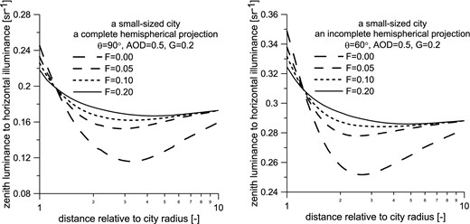
Zenith luminance relative to horizontal illuminance computed for small-sized city. Leftmost plot is for complete hemisphere, while rightmost plot is for the field of vision with 2θ limited to 120°.

Figure 7.

The same as in Fig. 6, but for a large-sized city.

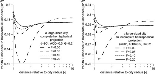
We have depicted the ratio of [B(θ)/D] as a function of distance and shown that the curves are similar in both cases, i.e. for complete and incomplete hemispherical projections. The only differences are the amplitude of the function and its steepness at small distances from the city. The same is accurate for large-sized cities (see Fig. 7) with exception that the ratio of zenith luminance to horizontal illuminance approaches its asymptotic behaviour 1–2 city radii from the city edge. This finding is not unexpected since the characteristic size of the city in Fig. 7 is five times larger than that in Fig. 6. The curves depicted in Figs 6 and 7 may change with optical properties of aerosol particles, especially with asymmetry parameter (ASY). It has to be noticed that ASY characterizes the spatial redistribution of scattered radiation. The most typical aerosol properties ASY = 0.8 and SSA = 0.9 were used in our model calculations, where SSA is so-called single scattering albedo of aerosol particles.

However, a limiting factor for making the inversion procedure successful is a temporal optical stability of the atmosphere at all distances. Fortunately, angular behaviour of city emission function does not change from day to day, thus a targeted field experiment can be repeated many times until the stable conditions are reached. Once the radiant intensity is determined as a function of the zenith angle, it can be used for a modelling in any time and under arbitrary meteorological conditions depending on a computational tool used for numerical modelling.

5 RESULTS

The comparative measurements using two cameras with different FOV were made in the vicinity of Bratislava city during the nights of 2014 May 21 and May 22. The measurements started before midnight at about 10:00 pm and finished not later than at 1:00 am. The sky conditions were not stable with high cirrus clouds, however, the meteorological situation has improved as the measurement continued. The atmospheric conditions were characterized by particulate matter PM₁₀ ranging from 15 to 30 μg m⁻³ and relative humidity not exceeding 65 per cent. PM₁₀ characterizes suspended particulates smaller than 10 μm in aerodynamic diameter. The values below 50 μg m⁻³ can be classified as low pollution level. This is a reason for why the sky scans were quite dark as documented in Fig. 8.

Figure 8.

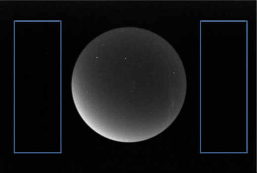
Typical sky brightness distribution near Bratislava city after removal of very bright objects. However, we have adjusted the contrast and brightness artificially to stress the effects of intensified brightness in the south-west quadrant due to light emissions from Bratislava city. Blue boxes on a photosensitive chip are used to read zero level signal.

Experimental ratios of zenith brightness to horizontal irradiance are depicted in Fig. 9 as a function of distance similar to what we have determined theoretically in Figs 6 and 7. The distance is measured relative to the city radius. Since near-horizon brightness are excluded from filtered data, the amplitudes of the experimental ratios are slightly higher than those plotted in leftmost part of Fig. 7. Horizontal irradiances for B-channel were also not taken into consideration due to high experimental errors. The measured profile of B(θ)/D suggests that F is as low as 0.1. Instead of data vector B(θ)/D we have only dealt with zenith brightness, since these data are obtained correctly for all red (R), green (G) and blue (B) channels, also with much simpler minimization routines than those for B(θ)/D.

Figure 9.

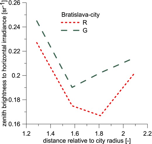
Zenith brightness to horizontal irradiance as determined experimentally near Bratislava city.

The ground reflectance of territory near Bratislava is known to be about 0.2 in late spring, thus we were able to use a simplified retrieval concept based on equation (4). This equation represents a convenient approach for determining the fraction of the light radiated directly into the upward hemisphere, since the minimization routines are exclusively based on zenith brightness data (i.e. SQM-like data). Input data were read from R, G, B channels separately, and result in F_B = 0.120 ± 0.054, F_G = 0.092 ± 0.030, and F_R = 0.108 ± 0.052. Relatively high F_B compared to F_G and/or F_R does not mean that Bratislava city emits a lot in blue. Instead, it can be an effect of intensive scattering by aerosol particles that are spread over Bratislava city and can scattering a large portion of light beams toward sky even if they are originally directed to the ground. In addition, F_B relates upward to total emissions, both only evaluated in blue part of the spectrum. In principle, the broad-band uplight should be determined as follows:

\begin{equation} \tilde F = \frac{{\sum\nolimits_{i = 1}^3 {w_i F_i } }}{{\sum\nolimits_{i = 1}^3 {w_i } }}, \end{equation}

(7)

where indices i = 1.3 are used for blue (1), green (2) and red (3), and

\begin{equation} w_i = \int_i {S_i \left( \lambda \right)} J\left( \lambda \right){\rm d}\lambda \end{equation}

(8)

is a weight that is an integral product of the spectral sensitivity S_i(λ) of blue (alternatively green or red) filter and the spectral emission function J(λ), i.e. the spectrum of a city. If city emissions are low in blue, then the corresponding weight w₁ is also low, implying F_B contributed to |$\tilde F$| only negligibly. The radiance data we have used in computational routines are plotted in arbitrary units and presented in Fig. 10. An elevated zenith radiance was measured 25–35 km from Bratislava city due to presence of local light source, in fact Galanta city. The minimization runs were therefore limited to distances below 23.2 km, which is the sixth measuring place.

Figure 10.

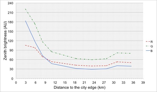
Zenith brightness in Bratislava surroundings plotted in arbitrary units as a function of distance from the city edge. Elevated values at distances above 25 km are due to emissions from Galanta city.

Our experiments were complemented by a field campaign in Los Mochis city, Mexico, aiming to analyse data from a territory with only one dominant light source. Basically, Los Mochis is well isolated, thus the zenith brightness is not influenced by a parasitic light from other cities. The optical measurements were made on 2014 April 2 and the results are plotted in Fig. 11 using arbitrary units. Variation of zenith brightness in the city territory is due to heterogeneity of public light distribution, while a local peak 8 km away the city is an effect of street lighting. This is produced due to the luminaires that are arranged along the way out of town. The uplights we have obtained for different parts of the spectrum: F_B = 0.21 ± 0.10, F_G = 0.21 ± 0.10 and F_R = 0.15 ± 0.06 that are higher values than those found for Bratislava. It indicates an inadequate shielding of direct upward emissions from a considerable fraction of lamps and from other light sources. Evaluating the uplights from Los Mochis relative to those from Bratislava gives the ratios: F_B(LM)/F_B(B) = 1.75, F_G(LM)/F_G(B) = 2.28 and F_R(LM)/F_R(B) = 1.39. An amplification of F_G by a factor of 2 or even more could be due to enhanced emissions to low elevation angles from green light sources, such as HPS, LPS and mainly advertisement boards.

Figure 11.

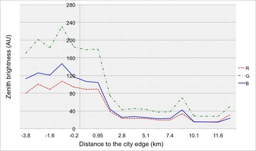
Zenith radiance in Los Mochis surroundings plotted in arbitrary units as a function of distance from the city edge. A local peak at distance of 8 km is due to street lamps outside the city.

Equations (4) and (6) can be also used to generate synthetic data of zenith radiance in the case both F and J(λ) are known for a monitored city. Each filter used must be known to apply this spectral sensitivity. However, the formulae (13)–(16) in Kocifaj & Solano Lamphar (2014) only approximate the full integrals introduced ibidem. Here we have used complete integral forms rather than approximations to determine uplight from zenith brightness data.

6 CONCLUSIONS

The emissions from ground-based cities or towns propagate in the atmosphere as a scattered light and cause an illumination of otherwise dark places. There are huge uncertainties in many properties of city lights, such as spatial distribution, spectral and directional characteristics of single lights and their interactions with the surrounding environment. While virtually unidentifiable, bulk light signal from a ground-based light source is fairly unknown due to the fact that it is submerged by the signals of a myriad of others. Because of their varied properties, interest has fermented recently in rapidly detecting and characterizing the superposition of light emissions from urbanized zones or large metropolitan regions. Because of the rapid development in the field and multidisciplinary nature of the topic, nowadays there is a substantial demand in retrieval of the fraction of light (F) radiated directly into the upward hemisphere.

In 2014 Kocifaj & Solano Lamphar have developed a contactless remote sensing method to extract F from ground-based observations of a clear sky. This time we have used and validated the method on a set of experiments made in Slovakia and Mexico. The method benefits of easy concept and use of a simple fisheye camera. Based on camera-specific projection and sensitivity functions the RAW images were analysed in order to retrieve zenith brightness B and cosine-projected irradiance D, which is a dedicated integral over all illuminated pixels. The advantage is that one picture contains information on both B and D, but the method presented here is only applicable under optically stable atmospheric conditions. Since the statistically averaged radiant intensity distribution is more-or-less stable for a given city, the field experiments can be repeated until the reliable solution is found.

There exist also approximate theoretical method indispensable in express analysis of zenith brightness data for which a vast data base already exists for many locations worldwide. This method allows one to reduce significantly the computational time and to apply fast inversion of SQM-like data to determine fraction F of the light radiated directly into the upward hemisphere. The presented approach also benefits from its wide applicability to different data achieved by different instruments, including fisheye lenses with incomplete hemispherical view.

The experimental data gathered in the vicinity of Bratislava city show that uplight F is about 0.1, implying that the direct upward emissions are lower than those in Los Mochis, and, most of the direct upward emissions are aimed at low angles above the horizon, having higher impact on skyglow at distant sites. Los Mochis emits two times more efficiently to the upper hemisphere compared to Bratislava. It is most probably due to poorly shielded luminaires and a public lighting system that might require a better design.

For the future, we prefer to analyse zenith radiance and horizontal irradiance separately since these two data sets form a complementary base with increased information content. It is because B as a function of distance d is similar to that of D(d), thus implying that a small perturbations applied on any of these two data functions may induce quite large response in the solution found. Both B and D can be determined in arbitrary units, thus no special calibration is necessary. Nevertheless, all elements of data vector should be obtained by the same device. The method developed here allows for adaptive FOV – it can help to avoid direct light emissions, e.g. near city edge. To extract a correct value of F from SQM-like data, the optical properties of the local atmosphere as well as the fraction G of the light that is isotropically reflected from the ground are required.

We conclude that the retrieval method is fairly good trade-off between complex indirect theoretical techniques and expensive direct monitoring of upward emissions from e.g. airplanes. Usually a few field campaigns are necessary until a reliable data are gathered. Although our experimental study was directed toward the reconstruction of Garstang's parameters, the methodology suggested is potentially applicable to any analytical function that is parametrized through F and G. Optical method used in this paper is a desirable technology for detection, primarily because such technology is rapid, the components are inexpensive and the techniques can be automated, requiring no highly specialized devices.

This work was supported by the Slovak Research and Development Agency under contract No: APVV-14-0017. HASL received a support from the National Council of Science and Technology of Mexico under the project Cátedras CONACYT # 2723. MK furthermore acknowledges the Slovak National Grant Agency VEGA (grant No. 2/0002/12).

REFERENCES

Alvarez del Castillo

E. M.

Crawford

D. L.

Davis

D. R.

Schwarz

H. E.

Astrophysics and Space Science Library

Light Pollution: The Global View

2003

284

Dordrecht

Kluwer

49

Aubé

M.

Franchomme-Fosse

L.

Robert-Staehler

P.

Houle

V.

Proc. SPIE, 5890

2005

248

Aubé

M.

Roby

J.

Kocifaj

M.

PLoS ONE

2013

8

e67798

Bukowiecki

N.

Kittelson

D. B.

Watts

W. F.

Burtscher

H.

Weingartner

E.

Baltensperger

U.

J. Aerosol Sci.

2002

33

1139

Chepesiuk

R.

Environmental Health Perspective

2009

117

A20

Cinzano

P.

Castro

F. J.

Mem. Soc. Astron. Ital.

2000

71

251

Cinzano

P.

Falchi

F.

MNRAS

2012

427

3337

Cinzano

P.

Falchi

F.

Elvidge

C. D.

Baugh

K. E.

MNRAS

2000

318

641

Cinzano

P.

Falchi

F.

Elvidge

C. D.

MNRAS

2001

328

689

Coffin

D.

DCRAW: Decoding Raw Digital Photos in Linux

2008

Available at: http://cybercom.net/dcoffin/dcraw

Craine

E. M.

Preliminary Experiments Using a Digital Camera to Measure Commercial Light Sources

2007

Tucson

International Dark Sky Association

Elliott

I.

Irish Astron. J.

1981

15

58

Falchi

F.

Thesis, Univ. Milan

1999

Falchi

F.

Cinzano

P.

Elvidge

C. D.

Keith

D. M.

Haim

A.

J. Environmental Management

2011

92

2714

Fliegel

K.

Havlin

J.

SPIE, 7443, 74431Q

2009

, Proc.

Garstang

R. H.

PASP

1986

98

364

Garstang

R. H.

PASP

1991

103

1109

Garstang

R. H.

Mem. Soc. Astron. Ital.

2000

71

Hoag

A. A.

Schoening

W. E.

Coucke

M.

PASP

1973

85

503

Horvath

H.

Atmos. Environment

1995

29

241

Horvath

H.

J. Quant. Spectrosc. Radiat. Transf.

2014

139

3

Joseph

J.

Kaufman

Y.

Mekler

Y.

Appl. Opt.

1991

30

3047

Kerola

D. X.

MNRAS

2006

365

1295

Kirschbaum

C.

Schwarz

H. E.

Astrophysics and Space Science Library

Light Pollution: The Global View

2003

284

Dordrecht

Kluwer

201

Kocifaj

M.

Appl. Opt.

2007

46

3013

Kocifaj

M.

Solano Lamphar

H. S.

J. Environmental Management

2013

127

300

Kocifaj

M.

Solano Lamphar

H. S.

MNRAS

2014

439

3405

Kollath

Z.

J. Phys.: Conf. Ser.

2010

218

012001

Kollath

Z.

Kranicz

B.

Quant. Spectrosc. Radiat. Transf.

2014

139

27

Luginbuhl

C.

Duriscoe

D.

Moore

C.

Richman

A.

Lockwood

W.

Davis

R.

PASP

2009

121

204

Middleton

W. E. K.

Vision Through the Atmosphere

1968

Toronto

University of Toronto Press

Mishev

D.

Remote Sensing of the Earth from Space

1985

Moscow

Mir

(in Russian)

Rich

C.

Longcore

T.

Ecological Consequences of Artificial Night Lighting

2005

Island Press, Washington, DC

Schnitt

S.

Ruhtz

T.

Fischer

J.

Hölker

F.

Kyba

C. C. M.

Sensors

2013

13

12166

Shiffrin

K. S.

Kozhaev

D. A.

Optics of the Ocean and the Atmosphere

1972

Leningrad

Nauka

210

Smith

M.

Nature

2009

457

27

Solano Lamphar

H. S.

Kundracik

F.

Lighting Res. Technol.

2014

46

20

Son Hosseini

S.

Nasiri

S.

IAU Special Session

2006

5

24

Astronomy for the Developing World. Prague, Czech Republic

Wuller

D.

Gabele

H.

Electron. Imaging Conf.

2007

6502

1