Roadway Lighting Retrofit: Environmental and Economic Impact of Greenhouse Gases Footprint Reduction

Abstract

Roadway lighting retrofit is a process continuously developed in urban environments due to both installation aging and technical upgrades. The spectacular example is replacing the high intensity discharge (HID) lamps, usually high pressure sodium (HPS) ones, with the sources based on light-emitting diodes (LED). The main focus in the related research was put on energy efficiency of installations and corresponding financial benefits. In this work, we extend those considerations analyzing how lighting optimization impacts greenhouse gas (GHG) emission reduction and what are the resultant financial benefits expressed in terms of emission allowances prices. Our goal is twofold: (i) obtaining a quantitative assessment of how a GHG footprint depends on a technological scope of modernization of a city HPS-based lighting system; and (ii) showing that the costs of such a modernization can be decreased by up to 10% thanks to a lowered CO${}_2$ emission volume. Moreover, we identify retrofit patterns yielding the most substantial environmental impact.

1. Introduction

Retrofitting a roadway lighting is a process continuously developed in urban environments due to installations aging and technical upgrades. The common example is replacing high pressure sodium fixtures with LED, plasma or induction ones (the last two also belong to gas discharge sources) [1] and involving various hardware modules (e.g., occupancy sensors) enabling lighting control [2]. The main problems being analyzed in the related research were reducing energy consumption, improving illumination quality [3], optimizing investment and maintenance costs [4].

It is worth noting that financial optimization of roadway lighting solutions applies also to such non-trivial cases as road tunnel illumination [5,6].

To support retrofit related optimization, a range of computing approaches are proposed including graph-based modeling of lighting systems [7] or evolutionary algorithms [8].

While the computational, technological and financial aspects of lighting design/retrofit are commonly discussed in the literature, a detailed analysis of an environmental impact of lighting system modernization is rather rarely present in the domain research [7,9,10].

To go beyond the obvious fact that a reduced power usage leads to a decreased GHG footprint, we made both qualitative and quantitative analysis of how using advanced lighting solutions influences a greenhouse gases emission. Moreover, we analyzed economic benefits resulting from a lowered CO${}_2$ emission, showing that the retrofit investment costs can be effectively reduced by up to 10%.

Similarly, as for the roadway lighting optimization improving energy efficiency, we distinguished three possible retrofit scopes.

• HID to LED replacement: The only action is installing LED sources in places of HID ones. An upgraded installation is not additionally adjusted (e.g., by fixture dimming).
• Optimization of an installation: The scope of this process may vary depending on a particular case, from appropriate lamp dimming and changing the fixture mounting angles or arm lengths to displacement of selected poles. Note that, due to the certain limitations of HID sources, an HID-based installation should be migrated to LEDs prior to luminous flux adjustments.
• Introducing control systems: This most advanced approach to upgrading a lighting installation performance can be made at several levels. In the simplest case, it relies on scheduling, where luminous fluxes change according to the predefined rules at fixed hours [11,12] and do not depend on actual environment conditions such as traffic flow intensity, ambient light level or weather conditions. In the advanced scenarios, a lighting installation performance is adjusted dynamically on the basis of environment state’s changes reported by a telemetry layer (induction loops, weather and occupancy sensors, etc.).

As CO${}_2$ and other GHG emissions are linearly dependent on the energy usage, we made a parallel analysis of both. This analysis was based on the real-life retrofit, the details of which are presented in Section 3.

In this work, we propose the way of linking a quantitative analysis of financial aspects of a lighting installation retrofit with considerations on an environmental influence (in terms of CO${}_2$ emission) of such a modernization. Thus, an environmental influence can be included quantitatively in a retrofit strategy planning. The goal of this work was threefold: (i) finding an impact of the above three retrofit approaches on the resultant CO${}_2$ emissions, in terms of their volumes; (ii) finding which lighting classes [13] contribute the most, in the context of emission reduction, to the final financial gains; and (iii) how the reduced CO${}_2$ emissions change the annual costs of a lighting installation performance.

This article is structured as follows. In Section 2, we overview the approaches listed above and present estimations of expected energy savings for each of them. Section 3 contains the case study of the retrofit carried out in Cracow, Poland. Beginning with the presentation of its background, we show how particular strategies (i.e., relamping, adjusting lighting installations, and introducing control capabilities) decrease power usage and thus the GHG emission volumes. The extrapolation of results to the scale of a lighting system of the entire city is also presented. Further, we convert CO${}_2$ emission volumes to the costs related to the corresponding emission allowances. We show that those costs can reach 10% of savings achieved thanks to decreased power usage. In Section 4, we discuss obtained results. The final conclusions are contained in Section 5.

2. Retrofit Strategies–State of the Art

In this section, the detailed overview of retrofit approaches enumerated in the previous section are presented. The relevant GHG emission reductions are expressed in terms of power reduction ratios as the GHG emissions can be simply obtained on this basis.

2.1. Light Sources Replacement

Replacing HID-based luminaires (in particular, the HPS sources) with LEDs is a common retrofit pattern. What is interesting, due to the significant financial benefits, the municipalities decide to install LEDs, even if the end of an HPS fixtures’ life cycle is not reached.

Typically, during an HID to LED migration, conversion charts provided by lamp vendors are used (see

Table 1. HID to LED conversion chart [14].

HID System	HID Wattage [W]	LED Wattage [W]	Savings
70 W Pulse MH	88	53	40%
100 W Pulse MH	129	53	59%
150 W Pulse MH	190	80	58%
250 W Pulse MH	291	156	46%
320 W Pulse MH	368	232	37%
400 W Pulse MH	452	309	32%
70 W HPS	85	53	38%
100 W HPS	115	53	54%
150 W HPS	170	103	39%
250 W HPS	300	183	39%
400 W HPS	465	309	34%

). Such a chart allows finding, for a given HID lamp’s power, a rough estimation of an equivalent (in terms of a desired luminosity) LED’s wattage to be installed.

Although the unit savings shown in Table 1 are, as mentioned, only the rough estimations supplied by a specific manufacturer, they express the order of magnitude of available power reduction ratios. For the considered example, those ratios vary between 32% and 59%. It is obvious that total power savings for any real-life case will depend on both the lighting system structure, i.e., the ratios of particular fixture types being retrofitted, and the installation’s size.

2.2. Lighting Design Tunning

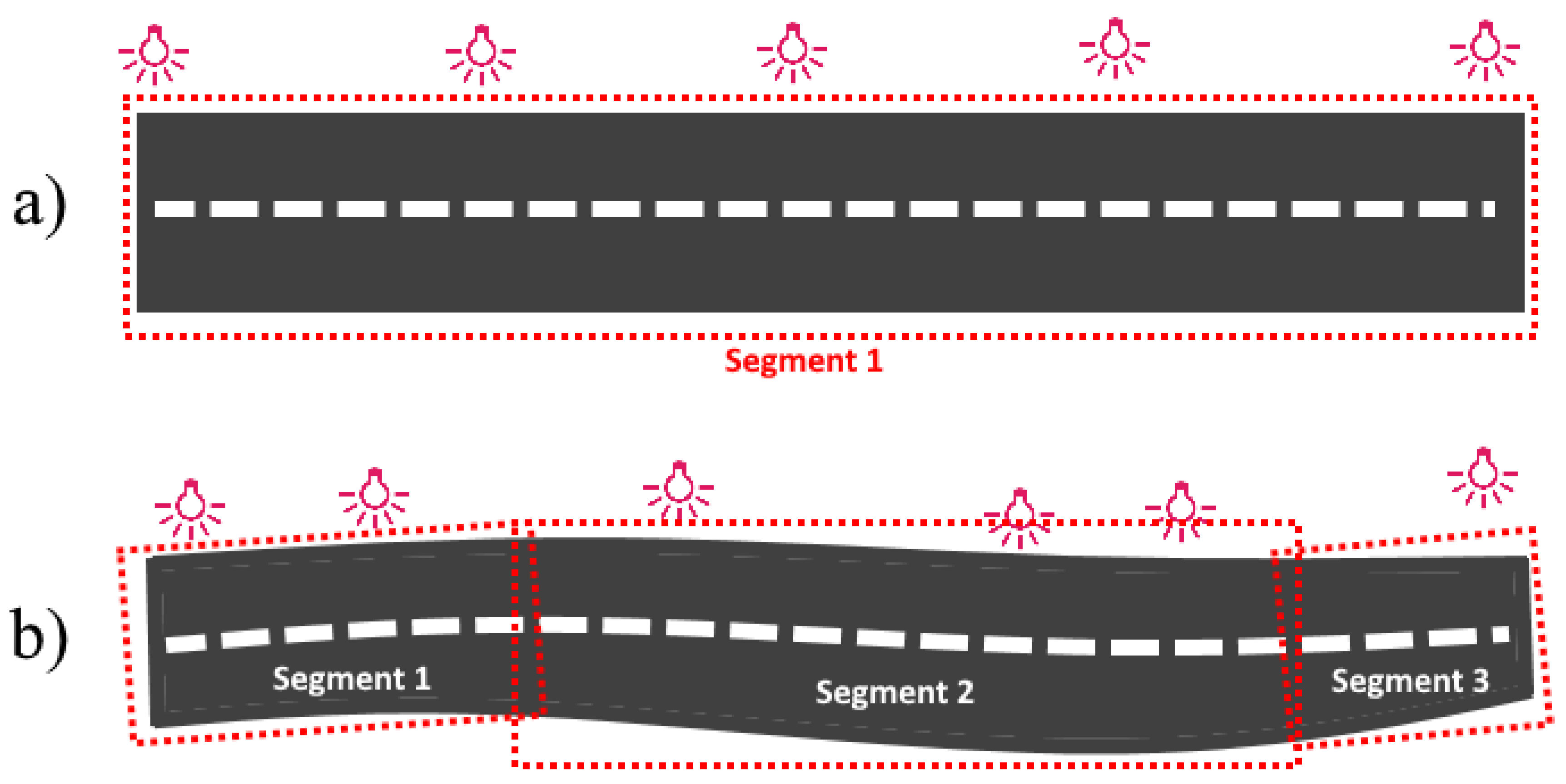
Power savings can be obtained thanks to a well suited lighting design. It is achieved by adjusting lamp parameters such as the fixture’s photometric solid, dimming, pole height, arm length, fixture’s mounting angles, etc. The above installation tuning may be done according to the either standard or customized design approach. In the first case, one assumes regularity and uniformity of a lighting situation, namely, a constant road width and evenly spaced luminaires (Figure 1a). In the second approach, an actual roadway layout is assumed (Figure 1b).

The former method makes an installation meet performance requirements imposed by a lighting standard and minimize power usage. This approach, as a multivariate optimization, requires advanced software tools capable of solving the problem in an acceptable time. It has to be noted that imposing uniformity of a lighting situation leads to over-lighting due to the conservative assumptions on the road width and lamp spacing.

The latter design scheme, relying on the different design paradigm, was introduced in the work [15]. In this approach, the lighting situation is regarded strictly as is, i.e., with its actual geometry recovered on the basis of GIS coordinates (Figure 1b). In addition, the coordinates of luminaires are taken from a GIS data repository. In such an approach, the lighting situation is no longer uniform, which means that neither road width is constant nor luminaires are distributed evenly along a road. Although this method implies a significant computational overhead (one has to analyze multiple road segments rather than a single roadway, as shown in Figure 1), the resultant installation’s configuration is designed in such a way that over-lighting is minimized. As shown in [15,16], the customized design method reduces a power usage by 15% compared to the standard approach described above.

2.3. Control

While assessing lighting class selection for a given street segment there are certain measurable coefficients that influence this process. One of them is traffic intensity, or volume. Depending on the number of vehicles passing, there could be up to three different lighting classes assigned. Varying lighting classes lead to different dimming settings of the luminaires, which results in energy savings. While assigning a lighting class, the maximum traffic volume should be considered. For such a class, power levels of the luminaires should be selected accordingly by means of photometric calculations. If information about a current traffic volume is available, then changing the classes for a given street segment can be performed efficiently [17,18], which leads to energy savings [19] and CO${}_2$ emission reduction.

Table 2. Different lighting control strategies and corresponding energy saving (lighting classes according CEN/TR 13201-1:2004). Any lighting class change is triggered by a varying traffic volume.

Control Strategy	ME2 [%]	ME3b [%]	ME4a [%]	Energy Saving [%]
Calendar	100	0	0	0
Statistics	46.5	15	38.5	24
Dynamic	27	14	59	34

presents the 24-h lighting class assignment structure and the comparison of obtained savings for various control approaches. The table is made for the arterial road with a dominant lighting class ME2.

Remark 1.

It should be noted that the new release of the standard CEN 13201 was issued in 2014 but its Polish localization was published two years later, in 2016. For that reason, the calculations presented below was initially made in accordance with CEN 13201:2004.

The analysis was based on 100 luminaires and one year worth of traffic data. The calendar control strategy assumes that ME2 is assigned regardless of an actual traffic intensity and lighting is turned on at sunset and turned off at sunrise, totaling 4292 on-hours. The dynamic assumes reading traffic intensity every 15 min. The lighting classes are adjusted accordingly which leads to the 34% energy saving comparing to the calendar approach. ME2 is used 27% of the time, while the lower class, ME3b, is assigned 14%, and ME4a 59%.

In some situations, a statistic approach is also used. In this case, the control is not based on actual traffic volume but on statistical analysis of its historical data records—separately for working days, holidays, Saturdays, and Sundays. Even though it is commonly used, it very often leads to lighting class violations because of a high traffic variability. An actual traffic volume can surpass the statistics based on historical or incomplete data. An example for the aforementioned arterial road is also presented for comparison. For more diverse road and street infrastructure, actual savings obtained by application of dynamic control are expected to be at the level of 27% [20].

The above findings regard CEN/TR 13201-1:2004. The current release of the standard (since 2014) alters number of regulations, lighting class names and their assignment methods, among others. It also introduces a notion of an adaptive control. This gives greater flexibility for dynamic control applicability. A comparison of energy savings achieved thanks to application of a dynamic control, made for a slightly larger and more representative area with variable, high volume traffic, is given in

Table 3. Dynamic lighting control energy saving for ME2 and M2 base lighting classes; comparison between CEN/TR 13201-1 releases 2004 and 2014.

Standard	ME2/M2 [%]	ME3b/M3 [%]	ME4a/M4 [%]	Energy Saving [%]
CEN/TR 13201-1:2004	50	15	35	33
CEN/TR 13201-1:2014	8	32	59	46

. There are 210 luminaires installed, with the total power of 26,933 W. The total annual operation time is 4292 h. In this table, we compare the performance structure for both 2004 and 2014 releases of CEN/TR 13201-1. As can be seen, following the 2014 revision leads to significant savings, from 35% to 46%, which gives the motivation to upgrading a lighting infrastructure performance to the new release of the standard. It is mainly due to introduction of maximum traffic capacity indicator on which assignment of lighting classes is based now. The M2 class is assigned 8% of the time only.

The energy saving is also influenced by the traffic intensity parameters, in particular how often the data are read from sensors and how wide is the averaging time window [20].

3. Case Study

In this section, we analyze in depth the case of retrofit carried out in the city of Cracow, Poland. After making an overview of the lighting system being modernized and the structure of lighting classes of relevant roads (Section 3.1), we analyze how the power usage can be decreased by selecting a given retrofit approach (Section 3.2). Next, those savings are converted into the emission reductions (Section 3.3) and extrapolated to a scale of the entire city area (Section 3.4). In the last subsection (Section 3.5), we assess how a lower ${\mathrm{CO}}_2$ emission influences an ultimate financial balance.

Remark 2.

It should be stressed here that the emission values presented in this section depend strongly on emission factors which vary for different countries (for details, see [21]). For the purposes of this analysis, we assumed Polish emission factors [22], which are shown in

Table 4. Emission factors for Poland.

Gas	Factor Value [kg/MWh]
CO${}_2$	806
SO${}_2$	0.844
NO${}_x$	0.850
CO	0.260
Particulate matter	0.054

.

3.1. The Installation’s Setup

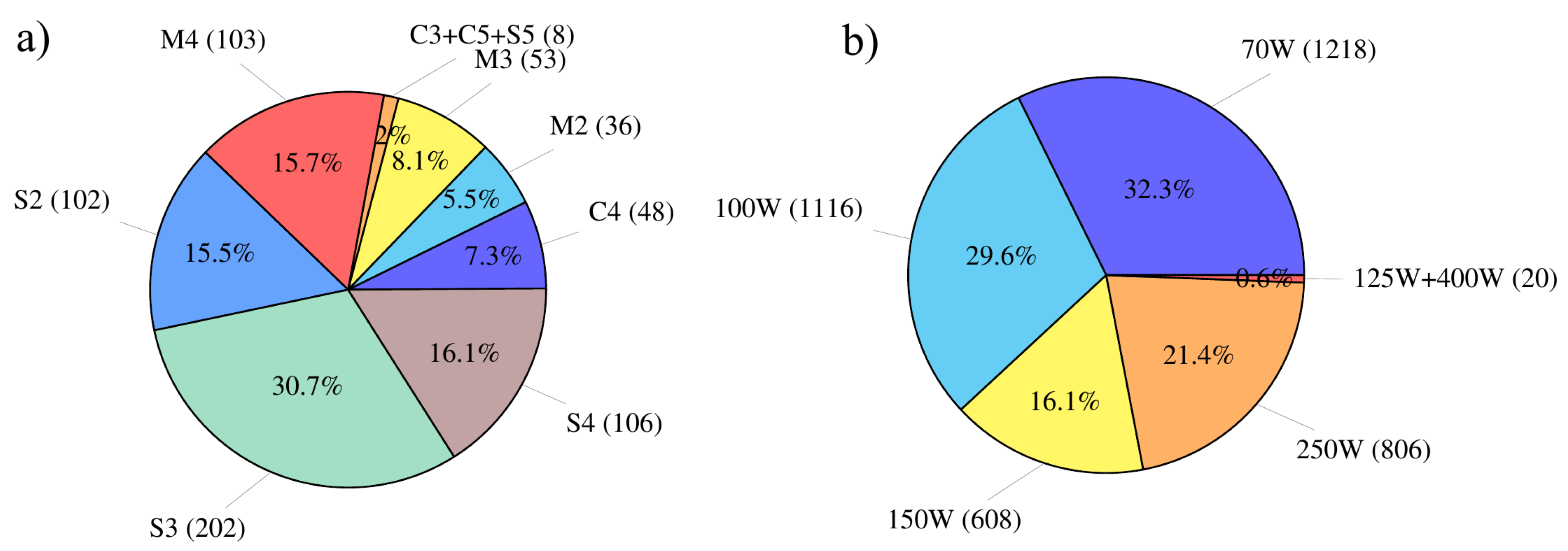
The modernization of a lighting system covered 3768 out of 80,000 luminaires installed in Cracow. Those sodium fixtures were replaced by LED sources (see Section 2.1). Additionally, newly installed LEDs were dimmed to adjust luminous fluxes to actual needs, defined by relevant lighting classes (see Section 2.2). The charts illustrating the considered system’s structure are shown in Figure 2 (the structure of lighting classes (Figure 2a) and powers of HID sources being replaced (Figure 2b)). The circuits were connected to 81 control cabinets.

3.2. Power Usage Optimization

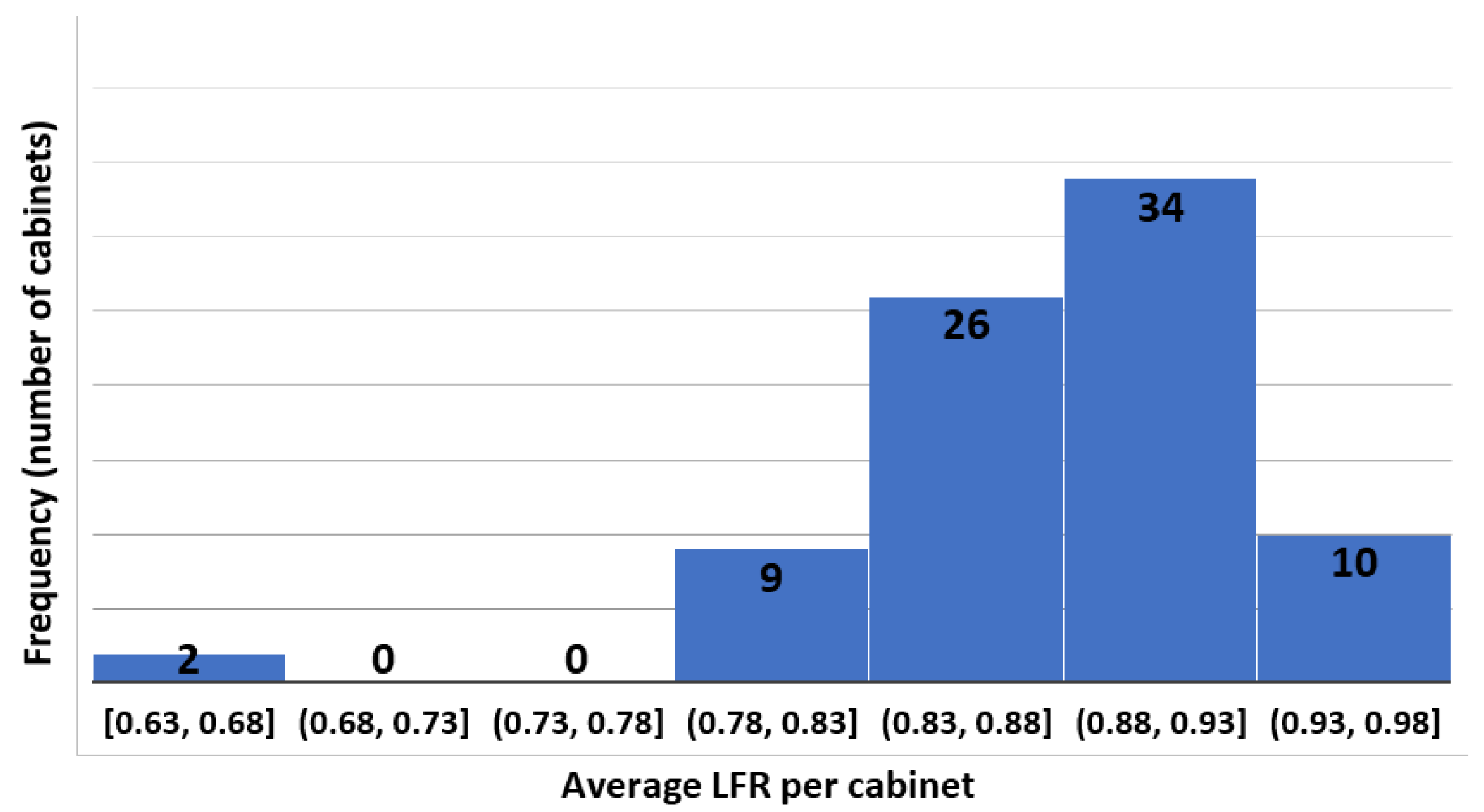
The total power of the initial, sodium-based installation was $P_{Na}$ = 311.9 kW. Replacing HID fixtures by non-dimmed LEDs reduced it to $P_{LED}$ = 183.2 kW, and dimming them brought finally $P_{LED}^{dim}$ = 157.8 kW. Average dimming per cabinet varied between 0.63 and 0.97 (where 0 denotes full dimming, i.e., a fixture being switched off, and 1 corresponds to a non-dimmed state). Frequencies of particular dimming ranges are shown in Figure 3.

Taking into account the total annual operation time of the lighting system T = 4292 h [18], the above powers give annual energy usages $E_{Na}$ = 1338.7 MWh, $E_{LED}$ = 786.3 MWh and $E_{LED}^{dim}$ = 677.3 MWh, respectively. Additionally, adding control capabilities to a lighting system reduces $E_{LED}^{dim}$ by 27% (see Section 2.3): $E_{LED}^{dim,ctrl}$ = 494.4 MWh.

3.3. Greenhouse Gas Emission Reductions

Table 5. The energy usage and GHG emissions corresponding to 3768 lighting points, for four setups: Na (sodium based–before retrofit), LED (relamping only), dimmed LEDs (after additional luminous flux tunning) and dimmed LEDs with control.

	Na	LED	LED Dimmed	LED Dimmed + Control
Power usage [kW]	311.9	183.2	157.8	115.2
Annual Energy consumption [MWh]	1338	786	677	494.4
CO${}_2$ emission [MT]	1079	634	546	398
SO${}_2$ emission [MT]	1.13	0.66	0.57	0.42
NO${}_x$ emission [MT]	1.14	0.67	0.58	0.42
CO emission [MT]	0.35	0.20	0.18	0.13
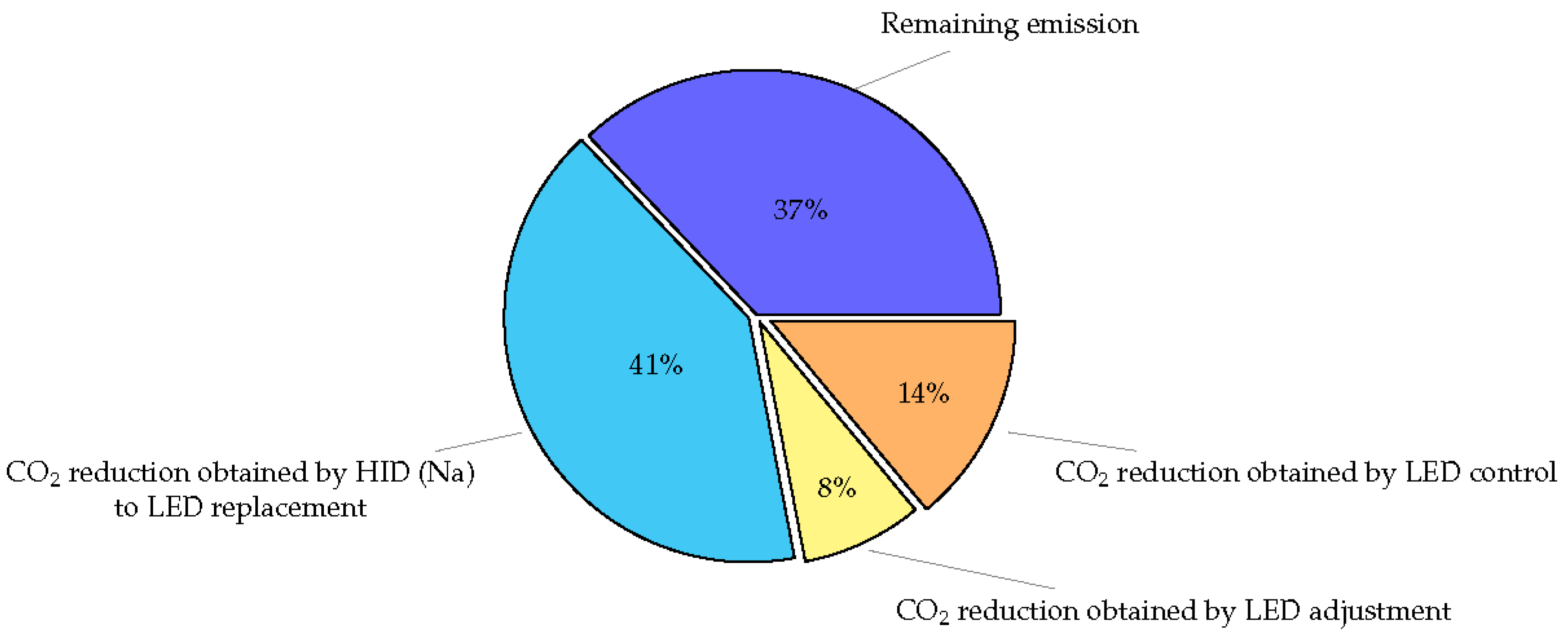
particulate matter [kg]	72	42	37	27

groups all data obtained in the previous subsection and presents the savings in terms of a GHG emissions reduction, as calculated according to the emission factors for Poland [22] (see Table 4). As shown, replacing HPS fixtures with LEDs gives the 41% reduction while adjusting LED dimmings brings additional 8%, thus reducing the GHG emission corresponding to sodium lamps by 49%. Introducing lighting control increases this ratio to 63%. Thus, finally, we obtain that 1 MT (metric ton) of CO${}_2$ (the same applies to other greenhouse gases) emitted when producing energy required by sodium vapor lamps is reduced to 0.37 MT of CO${}_2$ for an adjusted, controlled, LED-based lighting installation.

3.4. City-Scale Power and Emission Reductions

Having the reductions achieved for a representative set of lighting situations (in terms of lighting classes and fixture powers) (Table 5), we can estimate the total GHG emission reduction for the entire city with 80,000 luminaires. The results are shown in

Table 6. The estimated energy usage and GHG emissions corresponding to 80,000 lighting points, for four setups: Na (sodium based–before retrofit), LED (relamping only), dimmed LEDs (after additional luminous flux tunning) and dimmed LEDs with control.

	Na	LED	LED Dimmed	LED Dimmed + Control
Power usage [MW]	6.6	3.9	3.4	2.4
Annual Energy consumption [GWh]	28.4	16.7	14.4	10.5
CO${}_2$ emission [MT]	22,908	13,455	11,590	8461
SO${}_2$ emission [MT]	23.99	14.09	12.14	8.86
NO${}_x$ emission [MT]	24.16	14.19	12.22	8.92
CO emission [MT]	7.39	4.34	3.74	2.73
particulate matter [kg]	1535	901	776	567

.

Figure 4 gives a more intuitive view of the contributions brought by particular retrofit methods.

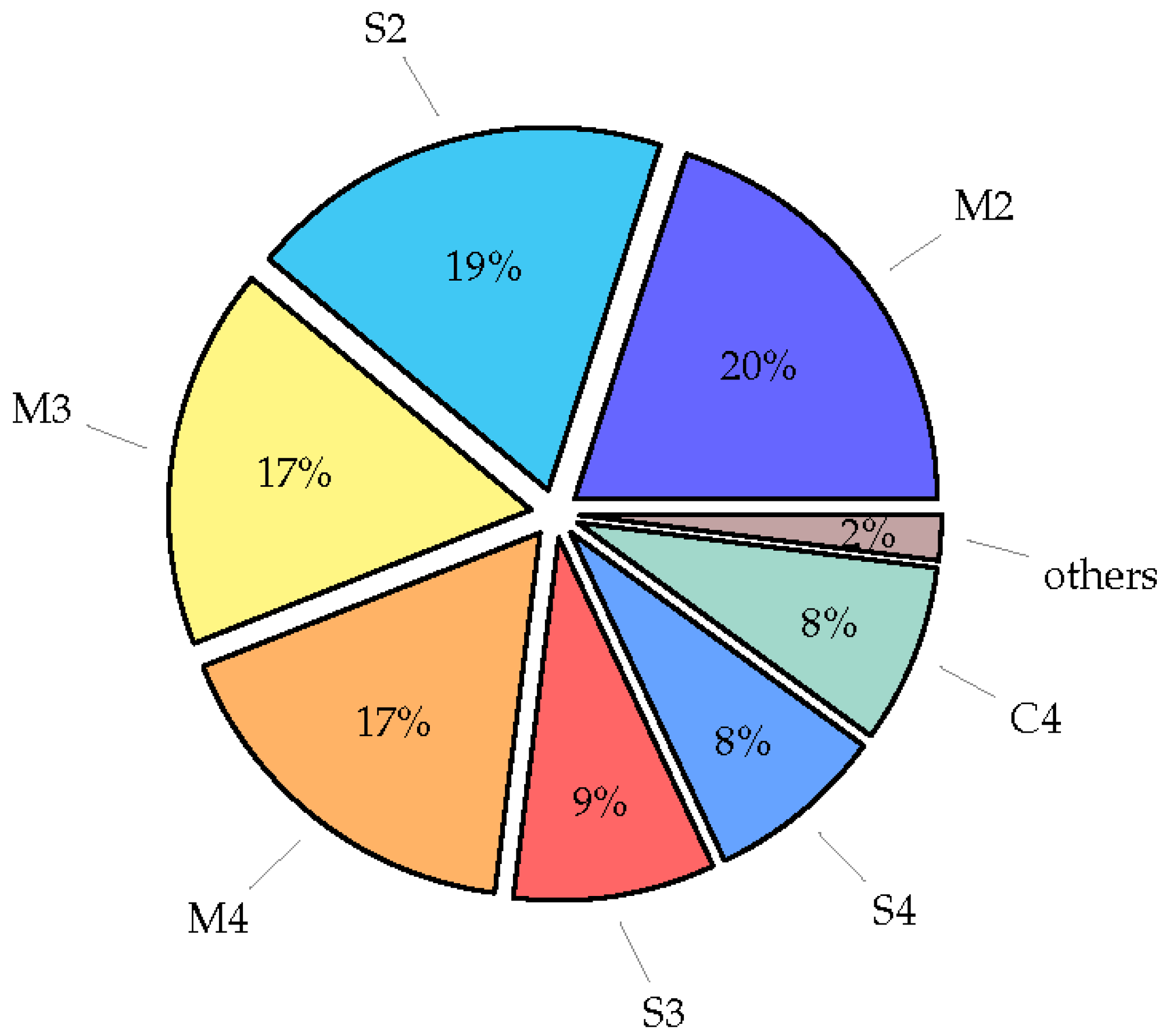
An interesting problem related to lighting system retrofit, in the context of GHG emission reduction, is finding the relation between a lighting class of a given area and a potential emission reduction. This relation can be obtained on the basis of statistical analysis of data gathered for a considered case. Finding this relation allows answering the question of which lighting installations should be upgraded first (e.g., in a situation of limited financial resources) to achieve the maximum environmental impact. Figure 5 presents an annual reduction of CO${}_2$ emission corresponding to the retrofit considered in this case study, broken down into contributions brought by particular lighting classes. As can be seen, the most GHG reduction was contributed by retrofitting roadways/areas of M2 and S2 classes.

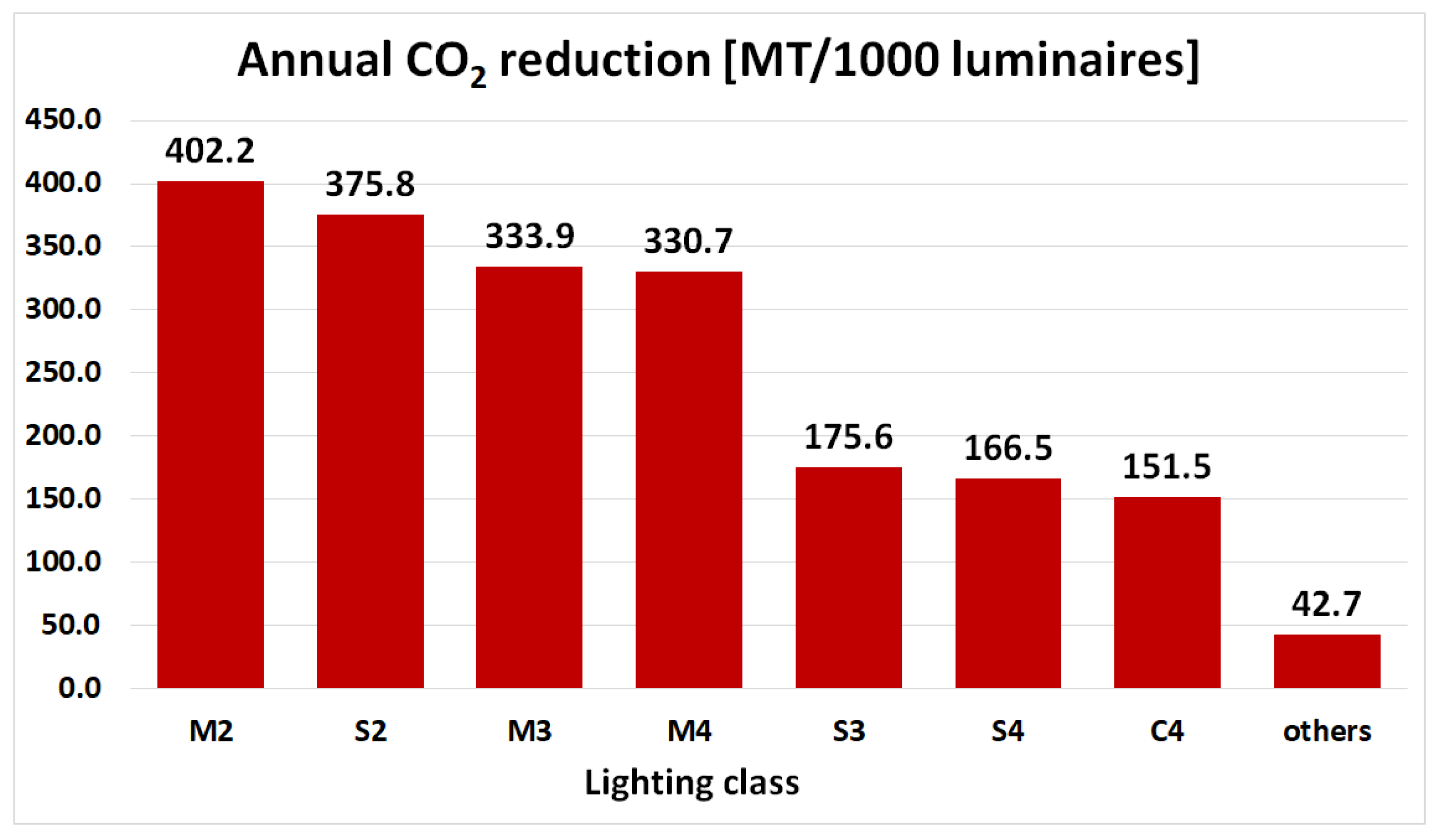
Figure 6 shows the above results in more tangible form, i.e., in terms of an annual CO${}_2$ emission reduction volume expressed in metric tons per 1000 luminaires.

3.5. Decreased CO${}_2$ Emission and Financial Savings

Let us compare now the direct financial benefits achieved thanks to the retrofit-based energy savings (i.e., reduced power consumption) and the savings derived from a reduced CO${}_2$ emission, computed on the basis of prices of European Union emission allowances (EEX EUA, or simply “EUA”) traded on secondary market. The former component is calculated for the average electricity price for non-household consumers for EU-28 (second half of 2017) which equals €0.14 per kWh [23]. In turn, the EUA price is assumed to be €17.00/MT [24].

The values presented in

Table 7. Annual energy savings and CO${}_2$ reduction in terms of financial benefits. The average electricity price €0.14/kWh for non-household consumers for EU-28 (second half of 2017) and the EUA price €17.00/MT were assumed. Results correspond to data in Table 6.

		LED	LED Dimmed	LED Dimmed + Control
Energy savings	[GWh]	11.7	14.0	17.9
	[€]	€1,641,895	€1,965,936	€2,509,484
CO${}_2$ reduction	[MT]	9453	11318	14,447
	[€]	€160,695	€192,409	€245,607

show that, besides the environmental impact, the CO${}_2$ reduction increases by 10% annual profits brought by a retrofit.

Remark 3.

The following simple reasoning shows that annual financial savings (S) increased by $\Delta =10\%$ (CO${}_2$-related component) can reduce an investment payback period (T) by 9%. Indeed, if C stands for the retrofit investment costs, then $T=C/S$. After increasing an S value by 10%, we obtain:

$$T^{\prime }=\frac{C}{S+\Delta ·S}=\frac{C}{1.1·S}=91\%T.$$

It should be remarked that, since an actual EUA price is subject to stock fluctuations this ratio can change (see

Table 8. Retrofit payback growth related to CO${}_2$ reduction vs. EUA price.

EUA Price [€/MT]	10.00	15.00	17.00	20.00
Retrofit payback growth	6%	9%	10%	12%

).

4. Discussion

Several comments related to the above analysis have to be made.

Volumes of GHG emissions presented in the previous section may be slightly different for other countries due to different structure of energy sources (see [25]) and different emission factors. For example, countries with an overwhelming share of nuclear plants in the total electricity production can have a lower CO${}_2$ emission factor than countries where most electric energy is produced in the coal plants.

As mentioned previously, although lighting class and luminaire power structures of the considered case (see Figure 2) are sufficiently representative for the presented analysis, one has to keep in mind that such an extrapolation estimates results rather than gives the precise values. Regardless, those numbers give a reasonable measure of an overall reduction of a GHG related pollution in the scale of the entire city.

The results shown in Figure 5 correspond to the roadway structure of the city of Cracow and may be subject to changes for a city having a different road network structure. Additionally, municipalities can apply other lighting class assignment policies resulting in dominance of high or low energy demanding classes.

A highly important issue for authorities planning lighting retrofit works are investment costs. One has to be aware that a final decision on retrofit strategy is usually a trade-off between financial constraints and other, non-fiscal (from the investor’s perspective) factors such as environment protection. The presented results shed light on how the latter can be taken into account when assessing an investment’s financial profitability.

In the presented considerations, we did not discuss maintenance costs of a lighting installation. They are another factor which leads to choosing LEDs [26]. It is worth mentioning that the total maintenance cost savings achieved thanks to upgrading 300 fluorescent tubes with 100 ballasts to LEDs is over $ 16,500 over an LED lifetime. For the case of HIDs, upgrading 100 bulbs to LEDs yields over $45,000 of the total maintenance cost savings, over an LED lifetime [27].

5. Conclusions

In this work, we considered how modernization of HPS-based lighting installations influences CO${}_2$ emission volumes related to urban roadway lighting. CO${}_2$ and other greenhouse gases emissions are linearly dependent on the energy usage so a parallel analysis of both was made. Our study relied on the real-life case of the retrofit made in the city of Cracow.

In our research, we show that:

• The highest contribution (41%) to the emission reduction was generated by relamping, i.e. replacing HPS fixtures by LEDs. The next factor (14%) was introducing an adaptive lighting control system. An important condition which was imposed on the control was that the resultant luminaire performances had to comply with the EN 13201-2 lighting standard [13]. In third place (8%) was preparing well suited lighting designs of installation being retrofitted.
• The most demanding lighting classes (i.e., having the least indices x for Mx, Cx, and Sx) contribute the most to an overall emission reduction. It should be noted, however, that this result cannot be replicable if, for a given city, a number of lighting points illuminating low classes, say M5 or C5, is predominant.
• The value of emission allowances (with the EUA price at the level of €17.00/MT) corresponding to the reduced CO${}_2$ emission volume, reached 10% of relevant energy savings. This rate yields the 9% reduction of a retrofit payback period.

The presented work links well defined, quantitative analysis of financial aspects of a public lighting retrofit investment with considerations on environmental influence of such a modernization. This link is obtained thanks to assessing the money savings corresponding to a reduced CO${}_2$ emission. Thus the environmental impact can be included quantitatively in the retrofit strategy planning. Moreover, for investments financed in the ESCO (Energy Service Company) model [28,29], we show that a payback period can be shortened by 9% (or even more, taking into account the current trend of the EUA price) thanks to incomes achieved due to the reduced CO${}_2$ emission.

References

- Jiang, Y.; Li, S.; Guan, B.; Zhao, G.; Boruff, D.; Garg, L.; Patel, P. Field evaluation of selected light sources for roadway lighting. J. Traffic Transp. Eng. 2018, 5, 372–385. [Google Scholar] [CrossRef]
- Cacciatore, G.; Fiandrino, C.; Kliazovich, D.; Granelli, F.; Bouvry, P. Cost analysis of smart lighting solutions for smart cities. In Proceedings of the 2017 IEEE International Conference on Communications (ICC), Paris, France, 21–25 May 2017. [Google Scholar]
- Hyari, K.H.; Khelifi, A.; Katkhuda, H. Multiobjective Optimization of Roadway Lighting Projects. J. Transp. Eng. 2016, 142, 04016024. [Google Scholar] [CrossRef]
- Jiang, Y.; Li, S.; Guan, B.; Zhao, G. Cost effectiveness of new roadway lighting systems. J. Traffic Transp. Eng. 2015, 2, 158–166. [Google Scholar] [CrossRef]
- Salata, F.; Golasi, I.; Bovenzi, S.; Vollaro, E.d.L.; Pagliaro, F.; Cellucci, L.; Coppi, M.; Gugliermetti, F.; Vollaro, A.d.L. Energy Optimization of Road Tunnel Lighting Systems. Sustainability 2015, 7, 9664–9680. [Google Scholar] [CrossRef] [Green Version]
- Peña-García, A.; Gil-Martín, L.; Hernández-Montes, E. Use of sunlight in road tunnels: An approach to the improvement of light-pipes’ efficacy through heliostats. Tunn. Undergr. Space Technol. 2016, 60, 135–140. [Google Scholar] [CrossRef]
- Sȩdziwy, A. Sustainable Street Lighting Design Supported by Hypergraph-Based Computational Model. Sustainability 2016, 8, 13. [Google Scholar] [CrossRef]
- Gómez-Lorente, D.; Rabaza, O.; Estrella, A.E.; Peña-García, A. A new methodology for calculating roadway lighting design based on a multi-objective evolutionary algorithm. Expert Syst. Appl. 2013, 40, 2156–2164. [Google Scholar] [CrossRef]
- Clinton Climate Initiative. Street Lighting Retrofit Projects: Improving Performance, while Reducing Costs and Greenhouse Gas Emissions. Available online: https://goo.gl/iV32FL (accessed on 21 January 2018).
- Molina-Moreno, V.; Leyva-Díaz, J.C.; Sánchez-Molina, J.; Peña-García, A. Proposal to Foster Sustainability through Circular Economy-Based Engineering: A Profitable Chain from Waste Management to Tunnel Lighting. Sustainability 2017, 9, 2229. [Google Scholar] [CrossRef]
- Schréder. Owlet. Available online: http://bit.ly/2Oz2uqk (accessed on 11 August 2018).
- Philips. CityTouch. Available online: http://www.lighting.philips.com/main/systems/lighting-systems/citytouch (accessed on 11 August 2018).
- Road Lighting. Performance Requirements, En 13201-2:2015; European Committee for Standarization: Brussels, Belgium, 2015.
- EAOTN. Area/Roadway–HID to LED Equivalency. Available online: http://bit.ly/2OxbOLA (accessed on 29 June 2018).
- Sędziwy, A. A New Approach to Street Lighting Design. LEUKOS 2015, 12, 151–162. [Google Scholar] [CrossRef]
- Sȩdziwy, A.; Basiura, A. Energy Reduction in Roadway Lighting Achieved with Novel Design Approach and LEDs. LEUKOS 2018, 14, 45–51. [Google Scholar] [CrossRef]
- Wojnicki, I.; Ernst, S.; Kotulski, L.; Sędziwy, A. Advanced street lighting control. Expert Syst. Appl. 2013, 41, 999–1005. [Google Scholar] [CrossRef]
- Wojnicki, I.; Kotulski, L. Improving Control Efficiency of Dynamic Street Lighting by Utilizing the Dual Graph Grammar Concept. Energies 2018, 11, 402. [Google Scholar] [CrossRef]
- Wojnicki, I.; Ernst, S.; Kotulski, L. Economic Impact of Intelligent Dynamic Control in Urban Outdoor Lighting. Energies 2016, 9, 314. [Google Scholar] [CrossRef]
- Wojnicki, I.; Kotulski, L. Empirical Study of How Traffic Intensity Detector Parameters Influence Dynamic Street Lighting Energy Consumption: A Case Study in Krakow, Poland. Sustainability 2018, 10, 1221. [Google Scholar] [CrossRef]
- United Nations Framework Convention on Climate Change. National Inventory Submissions 2018. Available online: https://bit.ly/2zcY3v5 (accessed on 9 August 2018).
- The National Centre for Emissions Management. Emission Factors for CO2, SO2, NOx, CO and Particulate Matter (In Polish). Available online: https://bit.ly/2npZjCq (accessed on 9 August 2018).
- Eurostat. Electricity Price Statistics. Available online: http://bit.ly/2Ou6Mzu (accessed on 13 August 2018).
- European Energy Exchange Group. European Emission Allowances (EUA). Available online: http://bit.ly/2Oue8CZ (accessed on 13 August 2018).
- United States Environmental Protection Agency. Greenhouse Gas Equivalencies Calculator. Available online: http://bit.ly/2Oug2DD (accessed on 6 August 2018).
- Nick Heeringa. Benefits of LED Retrofits—Lower Maintenance Cost. Available online: http://bit.ly/2JgFVlk (accessed on 24 October 2018).
- Patrick Clouden. Save Big On Maintenance Costs By Retrofitting Your Business Lighting to LED. Available online: http://bit.ly/2Jeopy5 (accessed on 24 October 2018).
- The European Parliament and The Council. Directive 2006/32/EC on Energy End-Use Efficiency and Energy Services and Repealing Council Directive 93/76/EEC. Available online: http://bit.ly/2Ox5dRa (accessed on 24 October 2018).
- Asian Development Bank. Led Street Lighting Best Practices. Available online: http://bit.ly/2Ox4Wh6 (accessed on 21 January 2018).
Figure 1.
The typical (a) and customized (b) approaches to photometric computations. In the former case, a roadway layout is uniform (averaged). In the latter, an actual roadway layout used in the computations is decomposed into multiple segments which are processed consecutively.
Figure 2.
(a) Numbers of lighting situations (in parentheses) in the retrofitted area, grouped by lighting classes. (b) Numbers of HID fixtures (in parentheses) being replaced in the retrofitted area, grouped by nominal power.
Figure 3.
The histogram representing frequencies (bar heights) of average luminaire luminous flux ratios per cabinet.
Figure 4.
The CO emission reduction structure. The full circle represents emission of a sodium vapor lamp.
Figure 5.
The annual CO emission reduction (full circle) broken down into ratios contributed by particular lighting classes [13].
Figure 6.
The annual CO emission reduction broken down into volumes (metric tons per 1000 luminaires) contributed by particular lighting classes [13].