


Abstract
The angular distribution of the light emitted from a city is an important source of information about public lighting systems and it also plays a key role in modelling the skyglow. Usually, the upwardly directed radiation is characterized through a parametrized emission function – a semi-empirical approach as a reasonable approximation that allows for fast computations. However, theoretical or experimental retrievals of emission characteristics are extremely difficult to obtain because of both the complexity of radiative transfer methods and/or the lack of highly specialized measuring devices.
Our research has been conducted with the specific objective to identify an efficient theoretical technique for retrieval of the emission pattern of ground-based light sources in order to determine the optimum values of the scaling parameters of the Garstang function. In particular, the input data involve the zenith luminance or radiance with horizontal illuminance or irradiance. Theoretical ratios of zenith luminance LV(0) to horizontal illuminance DV are calculated for a set of distances d that separate a hypothetical observer from the light source (a city or town). This approach is advantageous because inexpensive traditional equipment can be used to obtain the mean values of the Garstang parameters. Furthermore, it can also be applied to other parametrizable emission functions and to any measuring site, even one with a masked horizon.
1 INTRODUCTION
The emissions from artificial light sources can be observed as skyglow because of the scattering phenomena in the Earth's atmosphere. Many years ago, the overillumination of the night sky was only noticed in large metropolitan regions or in densely populated territories. Now, however, it is an environmental problem with serious consequences for the night environment (Falchi et al. 2011; Gaston et al. 2012). Astronomical measurements are usually affected considerably because the excessive lighting of the night is responsible for veiling luminance that reduces the contrast of stars on the night sky. Because the scattering efficiency increases with the growth in the volume concentration of scatterers, the skyglow is significantly intensified in the lower troposphere as a result of elevated aerosol content. It is well recognized that the concentration of aerosol particles peaks in the atmospheric boundary layer, while the molecular atmosphere extends to much higher altitudes. However, both aerosols and air molecules are equally important in modelling radiative transfer in the cloudless atmospheric environment.
Diverse algorithms have been developed and introduced with the aim of modelling skyglow depending on the optical properties of the ambient environment. Although the cloudless atmosphere can be approximately treated as a plane-parallel medium, the heterogeneity of ground-based light sources makes the theoretical solution of radiative transfer non-trivial because of three-dimensional geometry and the lack of information on the bulk emission function of a monitored urban agglomeration. Note that the bulk function is a collective effect of the elementary emission functions of all artificial private and public lights that are distributed in the studied area. On the one hand, the theoretical characterization of the emission function often involves complex computational techniques for heterogeneous topology of the studied environment. On the other hand, any experimental retrieval of this function is extremely difficult, or even impossible, to obtain. For instance, photometric measurements using aircraft are difficult to interpret because of varying atmospheric extinctions along different optical paths (Kyba et al. 2013). Also, the radiance data recorded by an optical device usually belong to some bounded area that is seen within the instrumental field of view. However, the bulk radiant intensity function is a weighted sum of all radiant intensities for all emitting pixels. Even if the measurements are made under well-controlled conditions, the data acquisition appears to be very expensive, and is thus unpractical for routine use.
To overcome the complexities of the experimental determination of a locality-specific emission function, a set of distinct models is suggested and is largely applied to many cities or urbanized regions. Various studies have attempted to analyse light pollution in order to locate the best astronomical sites (Walker 1970; Berry 1976; Pike 1976). These empirical or semi-empirical models use population data to estimate the emission function. Nevertheless, the first serious discussions and analyses of skyglow emerged during the 1980s, after Garstang (1984) introduced a model of the brightness of the nocturnal environment based on the luminance of the night sky. A subsequent improvement of the Garstang theory was undertaken two years later (Garstang 1986) and has been used often since that time. One of the most considerable advantages of Garstang's approach is that skyglow is interrelated with some atmospheric features that make the model more accurate, although it still uses the standardization of light output per capita based on semi-empirical estimations. In both cases, Garstang (1984, 1986) relied on the concept of Walker (1970) to check his results. Some later studies were carried out in order to allow calculations based on the curvature of the Earth (Garstang 1989a), to draw relations between city population and light pollution (Garstang 1989b) and to isolate the effect of dust in light-pollution data (Garstang 1992).
Many of the theoretical studies that have focused on the characterization of the upwardly directed urban beams rely on the Garstang models. Garstang's so-called optical emission function has been the principal technique used by light-pollution researchers (Garstang 1986; Cinzano, Falchi & Elvidge 2001; Kerola 2006; Luginbuhl et al. 2009; Kolláth 2010), making this approach almost standard in skyglow modelling. Thus, Garstang's approach is one of the fastest semi-empirical solutions and it is widely used to characterize light sources with an azimuthally averaged emission function. For instance, Cinzano et al. (2000) relied on the Garstang model (Garstang 1986) to prove that the effects of light pollution strongly depend on the direction of the upwardly emitted beams and the distance to the measuring point.
Indeed, for modelling purposes, it is very useful to determine the city emission pattern, and this is required as an input to many numerical tools. Therefore, it is of great interest in any method that can be used to retrieve scaling parameters for the Garstang function. In fact, indirect methods appear to be more attractive compared to other conventional direct methods because indirect techniques are usually cheaper and experimentally much easier to realize. In this paper, we develop a fast algorithm that is employed to determine the optimum values of the scaling parameters of the Garstang emission function. The input experimental data comprise the zenith luminance (or radiance) and the horizontal illuminance (or irradiance), which are both easily measured by traditional or specialized devices (Duriscoe, Luginbuhl & Moore 2007; Kolláth 2010). The concept of this paper is equally applicable to measuring sites with open and masked horizons (see the discussion in Section 4). Therefore, such an indirect remote sensing technique has the potential to be used routinely in determining the mean bulk emission function of ground-based light sources. While the atmospheric optical properties can constantly evolve, the emission function only changes slightly with time. Most obviously, the angular behaviour of upwardly emitted radiation reflects the changes in the composition and/or structure of artificial public lighting systems (e.g. after its reconstruction). For this reason, we can assume that the parametrization of the emission function is advantageous because it allows targeted computations for any city, assuming a real configuration and light output of luminaires.
Using the method presented in this paper, the emission function can be analysed separately for each light pollutant source. Although the exemplar derivations are made for the Garstang function, the solution concept shown here is also applicable to other parametrizable emission functions. However, we consider here the clear sky conditions that are favoured by astronomers.
2 MODELLING THE DIFFUSE COMPONENT OF SKY LIGHT
Ground-based light sources emit electromagnetic radiation in almost all directions. A fraction of light that is propagated downwards is either absorbed or reflected by the underlying surface. The reflected light is added to the amount of light emitted directly to the upward hemisphere (hereafter referred to as uplight), resulting in illumination of the lower atmosphere. The light beams propagated upwards undergo absorption and scattering processes that cause an intensity decay, but only the scattering phenomenon is responsible for the appearance of the diffuse light of a night sky. To make things even more complex, the diffuse light is further absorbed and scattered, forming a field of multiply scattered light. All these processes were studied intensively long ago for daylight (Hansen 1971; Hovenier 1971), showing that higher scattering orders become important, especially in cloudy atmospheres (Begum 2000; Platnick 2001). To find a satisfactorily accurate solution for the spectral sky radiances in a multiply scattering environment, the radiative transfer equation (RTE) has to be solved subject to boundary conditions (Thomas & Stamnes 2002). Recently, Cinzano & Falchi (2012) applied the RTE approach for the purposes of modelling light pollution.
In general, many problems that determine the light scattering in the Earth's atmosphere are solved in terms of RTE. For a plane-parallel model, the spectral radiance has been found to be an integral product of the so-called source function (Minin 1988, p. 35). This approach is applicable to diverse scattering media, even to densely packed dusty layers (Kocifaj et al. 2010). However, the numerical computations based on RTE can be time-consuming because of the iterative solution concept. Van de Hulst (1980) has experimented with several methods, showing that successive-order scattering (SOS) is convenient for thin atmospheres with optical depths ranging from 0 to approximately 1. Under such turbidity conditions, the SOS method is usually preferred because it is simple to use and the convergence is fast enough (because of low eigenvalues).
It is very advantageous to use SOS because it allows us to take a set of analytical approximations for a slightly polluted atmosphere and/or for short optical paths in optically thin media. In the cloudless atmosphere, it deals with trajectories with lengths not exceeding some tens of kilometres. Seidl et al. (1999) performed targeted experiments in the urban atmosphere of Vienna during daytime and found that the mean horizontal extinction coefficient varies between 0.02 and 0.1 km−1 in summer time. The contamination by aerosol particles is essentially high in this season. Accepting that emitted light is propagated predominately at inclined trajectories, the extinction measured along a beam path is considerably lowered. In such a case, SOS can be considered for distances up to almost 50 km, or even more.
3 THEORETICAL APPROXIMATIONS TO THE ZENITH RADIANCE AND LUMINANCE
In equation (8), we have used the substitution dτ = kext dh, in which τ is the optical thickness of the atmospheric layer that extends from the ground up to the altitude h. Even if it was not indicated exactly, τ is a function of both h and λ.
The use of equation (18) is advantageous because only a few measurements of |$I^{S}_{V^{\prime }}(z=0)$| are needed to retrieve a sought Garstang parameter. Basically, the luminance can be measured at two to three discrete distances from the light source. However, if more than one parameter is unknown or if the approximate equation (11) cannot be applied for any reason, then a more general minimization concept has to be applied to determine the mean values of the Garstang parameters. In our numerical experiment, we have used more exact computations based on the zenith luminance (equation 3), which is determined relative to the horizontal illuminance (equation 4). To obtain the ratio of |$I_{V^{\prime }}(z=0)/D_{V^{\prime }}$| no absolute values of luminance and illuminance are needed when measurements are made by the same device. Note that luminance can be also measured by means of a luxmeter if situated either in the image plane of a telescope or simply at the base of a black tube with a small field of view. Because |$I_{V^{\prime }}(z=0)$| is evaluated relative to |$D_{V^{\prime }}$|, the above-mentioned ratio changes slowly with distance and it is not necessary to have a device operating over several orders of magnitude (only the aperture has to be adjusted accordingly). This is an important issue for experimentalists, because traditional inexpensive equipment can be used routinely to determine the mean values of the Garstang parameters. By evaluating the ratio of luminance to illuminance, the effect of instrument constants (i.e. device-specific scaling factors) is efficiently suppressed or even fully removed. Thus, there is no problem with optical effects such as specular reflections from the glass.
4 NUMERICAL EXPERIMENT ON THE GARSTANG FUNCTION
The skyglow characteristics vary significantly with the type of artificial light and, in particular, with the angular features of its emission pattern. To demonstrate the optical behaviour of the night sky, we have performed a set of computations using the well-known Garstang emission function (Garstang 1986); see Fig. 1. This function accounts separately for a fraction of light radiated directly upwards (F) and a fraction radiated towards the ground, and consequently reflected to the upper hemisphere G × (1 − F). The Garstang model relates the luminous flux to the population living in the monitored region (i.e. it is assumed that the population produces an output of average lumens per habitant). Because the zenith luminance is determined relative to the horizontal illuminance, the information on lumens per habitant is not an important topic in this paper and plays a minor role in the solution concept presented here. Also, a bright patch (or a light dome) produced by extremely bright individual sites is scarcely identified near the zenith, so the zenith luminance to horizontal illuminance appears to be an appropriate concept for retrieval of the mean values of the Garstang parameters. The shapes of radiant intensity distributions parametrized through F and G are documented in Fig. 1.
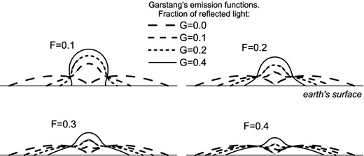
Emission function patterns computed in accordance with Garstang (1986), where F is the fraction of light directed upwards and G is the fraction of light that is isotropically reflected from the ground.
All numerical results shown here are obtained for Zmax = π/2, assuming a circular light source with a radius of 1 km. Although this radius corresponds to a small town rather than to a city, the theoretical model and computational method are valid for a planar light source with any radius. Therefore, in the general sense, a city can represent a ground-based light source of smaller size.
Theoretical ratios of zenith luminance LV(0) to horizontal illuminance DV are computed for a set of distances d that separate a hypothetical observer from the light source with a radius of 1 km. Based on these data, we have further determined LV(0)/DV at two distances: d = 1 km and d = 6 km. These distances are used to render different features of luminance scenes: while d = 1 km is located at the city border, d = 6 km is at a fairly large distance compared to the city radius. In this scenario, the zenith luminance is related to the sidescatter rather than to the backscatter. Also, the emissions towards low elevation angles become more important at d = 6 km, and thus we can expect a measurable difference between LV(0)/DV at 1 and 6 km. The ratios of LV(0)/DV computed in this way are independent of any absolute scaling parameter or instrumental constant. This is very advantageous from both experimental and interpretation points of view. On the one hand, it minimizes requirements imposed to both the experiment and the measuring device, and it also reduces complexities related to collecting the experimental data. On the other hand, the interpretation of such data in terms of the Garstang parameters or the optical turbidity of an atmospheric environment can be demonstrated in the following simple and straightforward example.
Let us consider two situations: a slightly turbid atmosphere characterized by low aerosol optical depth (AOD = 0.1) and a turbid atmosphere with elevated AOD = 0.5; see Tables 1 and 2.
Theoretical ratios of zenith luminance to horizontal illuminance computed for AOD = 0.1. The ratios are determined at d = 1 km and d = 6 km.a
| |$\frac{L_{V}(0)/D_{V} \;\mathrm{at\;distance}\; d = 1\; \mathrm{km \; from \; the \; light \; source}}{{L_{V}(0)/D_{V} \; \mathrm{at \; distance} \; d = 6\;\mathrm{km \; from \; the \; light \; source}}}$| | |||||
|---|---|---|---|---|---|
| G = 0.0 | G = 0.1 | G = 0.2 | G = 0.3 | G = 0.4 | |
| F = 0.0 | – | |$\frac{2.073e-01}{6.100e-02} = 3.40$| | |$\frac{2.073e-01}{6.100e-02} = 3.40$| | |$\frac{2.073e-01}{6.100e-02} = 3.40$| | |$\frac{2.073e-01}{6.100e-02} = 3.40$| |
| F = 0.1 | |$\frac{1.371e-01}{1.139e-01}= 1.21$| | |$\frac{1.621e-01}{1.096e-01} = 1.48$| | |$\frac{1.740e-01}{1.059e-01}=1.64$| | |$\frac{1.809e-01}{1.027e-01}=1.76$| | |$\frac{1.855e-01}{1.000e-01}= 1.86$| |
| F = 0.2 | |$\frac{1.371e-01}{1.139e-01}= 1.21$| | |$\frac{1.509e-01}{1.119e-01}= 1.35$| | |$\frac{1.602e-01}{1.100e-01}=1.46$| | |$\frac{1.669e-01}{1.083e-01}=1.54$| | |$\frac{1.719e-01}{1.067e-01}= 1.61$| |
| F = 0.3 | |$\frac{1.371e-01}{1.139e-01}= 1.21$| | |$\frac{1.459e-01}{1.127e-01}= 1.29$| | |$\frac{1.527e-01}{1.115e-01}= 1.37$| | |$\frac{1.582e-01}{1.105e-01}= 1.43$| | |$\frac{1.627e-01}{1.094e-01}= 1.49$| |
| F = 0.4 | |$\frac{1.371e-01}{1.139e-01}= 1.21$| | |$\frac{1.430e-01}{1.131e-01}= 1.26$| | |$\frac{1.480e-01}{1.124e-01}=1.32$| | |$\frac{1.523e-01}{1.116e-01}=1.36$| | |$\frac{1.560e-01}{1.109e-01}= 1.41$| |
a Zenith luminance LV(0) to horizontal illuminance DV for a circular light source with a radius of 1 km. The HPS lamps (NAV-4Y) are distributed homogeneously in the circular zone. AOD500 nm = 0.1.
Theoretical ratios of zenith luminance to horizontal illuminance computed for AOD = 0.5. The ratios are determined at d = 1 km and d = 6 km.a
| |$\frac{L_{V}(0)/D_{V} \; {\rm at \; distance} \; d = 1\; {\rm km \; from \; the \; light \; source}}{{L_{V}(0)/D_{V} \; {\rm at \; distance} \; d = 6\; {\rm km \; from \; the \; light \; source}}}$| | |||||
|---|---|---|---|---|---|
| G = 0.0 | G = 0.1 | G = 0.2 | G = 0.3 | G = 0.4 | |
| F = 0.0 | – | |$\frac{1.799e-01}{5.438e-02} = 3.36$| | |$\frac{1.799e-01}{5.438e-02} = 3.36$| | |$\frac{1.799e-01}{5.438e-02} = 3.36$| | |$\frac{1.799e-01}{5.438e-02} = 3.36$| |
| F = 0.1 | |$\frac{1.291e-01}{1.061e-01}= 1.22$| | |$\frac{1.447e-01}{1.028e-01}= 1.41$| | |$\frac{1.529e-01}{9.994e-02}=1.53$| | |$\frac{1.580e-01}{9.739e-02}=1.62$| | |$\frac{1.615e-01}{9.511e-02}= 1.70$| |
| F = 0.2 | |$\frac{1.291e-01}{1.061e-01}= 1.22$| | |$\frac{1.374e-01}{1.046e-01}= 1.31$| | |$\frac{1.434e-01}{1.031e-01}=1.39$| | |$\frac{1.479e-01}{1.018e-01}=1.45$| | |$\frac{1.514e-01}{1.005e-01}= 1.51$| |
| F = 0.3 | |$\frac{1.291e-01}{1.061e-01}= 1.22$| | |$\frac{1.343e-01}{1.052e-01}= 1.28$| | |$\frac{1.386e-01}{1.043e-01}=1.33$| | |$\frac{1.421e-01}{1.035e-01}=1.37$| | |$\frac{1.450e-01}{1.027e-01}= 1.41$| |
| F = 0.4 | |$\frac{1.291e-01}{1.061e-01}= 1.22$| | |$\frac{1.326e-01}{1.055e-01}= 1.26$| | |$\frac{1.356e-01}{1.049e-01}=1.29$| | |$\frac{1.383e-01}{1.044e-01}=1.32$| | |$\frac{1.406e-01}{1.038e-01}= 1.35$| |
a Zenith luminance LV(0) to horizontal illuminance DV for a circular light source with a radius of 1 km. The HPS lamps (NAV-4Y) are distributed homogeneously in the circular zone. AOD500 nm = 0.5.
By analysing Tables 1 and 2, we can observe that the ratio 1.29 can be found under two different turbidity conditions: case 1 with F = 0.3, G = 0.1 and AOD = 0.1; case 2 with F = 0.3, G = 0.1 and AOD = 0.5.
Note that observers usually have no information on AOD, but, as shown below, it is possible to infer this value from LV(0)/DV if measured at two different distances d. In the first case, we have LV(0)/DV = 0.1459 at the distance d = 1 km, while in the second case LV(0)/DV = 0.1356 is found at the same distance. This value is ≈10 per cent lower, as identified from the measured data when LV(0) is obtained relative to DV. A very similar decrease can be also found at the distance d = 6 km. When processing the spectral radiance/irradiance instead of luminance/illuminance, the variation in per cent will be even larger. This is because the luminance and illuminance are integrals over the visible spectrum, thus implying an efficient smoothing of any spectral features. Considering that the differences are ≈10 per cent for luminance or illuminance, the corresponding ratio for spectral quantities will be even higher. This analysis has shown that two situations with different values of AOD can be distinguished from one another using the measured ratios of LV(0)/DV (1 km) and LV(0)/DV (6 km).
The concept based on the ratios LV(0)/DV is also applicable to sites with a masked horizon. For instance, it is possible to consider a situation when the shielding by obstacles can block the light beams at elevations up to 20°. To eliminate the effects of all obstacles and to avoid beams propagated at low elevation angles, the measuring device can be embedded into a cylindrical mounting that masks all elevations below 20°. Then, to make the comparison of measured and theoretical data possible, we can simply integrate equation (2) from z = 0° to z = 70°. Consequently, the computed ratios of LV(0)/DV (listed in Tables 1 and 2 and shown in Figs 2–5) can be regenerated. It is then very easy and straightforward to use the new data in the same way as those computed for an open horizon.
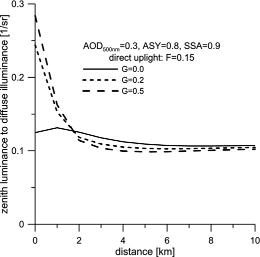
Zenith luminance to diffuse illuminance as a function of distance (d) to the light source. The computational parameters are as follows: city diameter = 2 km; AOD at reference wavelength 500 nm, AOD500 nm = 0.3; single scattering albedo of aerosol particles, SSA = 0.9; asymmetry parameter of aerosol particles, ASY = 0.8; direct uplight F = 0.15.
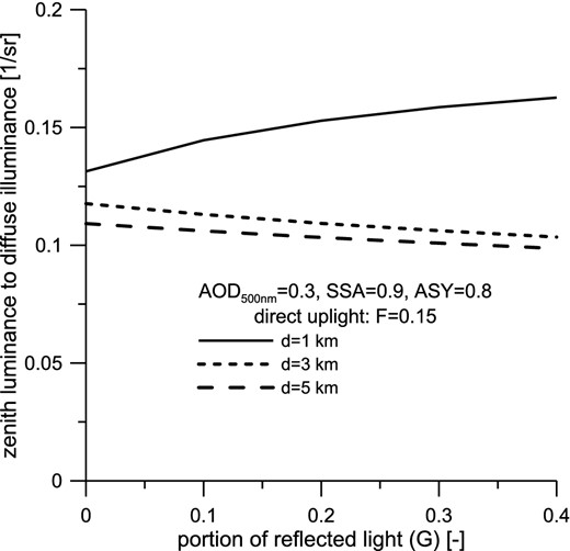
Zenith luminance to diffuse illuminance as a function of reflected light (G). The remaining parameters are the same as in Fig. 2.
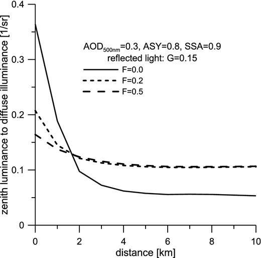
Zenith luminance to diffuse illuminance as a function of distance (d) to the light source with a radius of 1 km. The fraction of reflected light is G = 0.15, while the direct uplight is considered to be F = 0.0, F = 0.2 and F = 0.5 in a very extreme case.
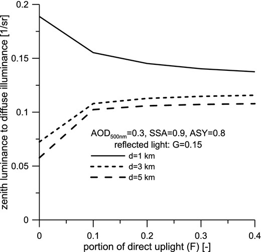
Zenith luminance to diffuse illuminance as a function of direct uplight. The remaining parameters are the same as in Fig. 4.
The above analysis can be very useful, especially when no all-sky scans/photographs are available and only zenith luminance is measured instead. To make the interpretation of the ratios LV(0)/DV more clear, it is convenient to draw more attention to the role of the Garstang scaling parameters: G and F. The effects of both are briefly summarized in the following subsections.
4.1 Reflected light
Fig. 2 presents the results obtained from the preliminary analysis of the ratio of zenith luminance to the diffuse illuminance LV(0)/DV as a function of distance to the light source. This concept is of great benefit from the point of view of experimentation and interpretation, as highlighted at the beginning of this section. The amount of uplight is fixed to 15 per cent. To demonstrate the effects of reflected light, we considered two extreme regimes: extraordinary reflective surfaces with G = 0.4 and totally black surfaces with G = 0.0. The intermediate case is characterized with G = 0.2. Considering extremely reflective surfaces (G = 0.4), the relative illuminance can exceed that for black surfaces by a factor of 3, if the measurements are made in the territory of a city. Typically, LV(0)/DV decreases rapidly when a hypothetical observer moves 1–2 km beyond the city border, except for the situation with G = 0. A small increment of LV(0)/DV over the 1-km city radius is observed only when the ground surface is absolutely black (i.e. when the underlying surface absorbs all the light directed downwards). In fact, this follows from the Garstang emission function that precludes any light beams to be directed towards the zenith (see Fig. 1). Most of the light signals recorded in the city centre are originated from backscatter or near-backscatter. The latter corresponds to the light emitted from luminaires that are situated at the city border. If the position of an observer changes from the centre of a city to its edges, the near-backscatter or sidescatter effects will contribute significantly to the signals detected. Then, the ratio LV(0)/DV will increase slightly. Fig. 3 shows the ratio as a function of G for three discrete distances d. If d = 1 km, the ratio has a constant increment, while the portion of reflected light is increased. This is because the reflected light is decisive inside the city but less important outside the city.
4.2 Uplight
Direct uplight causes major problems for astronomers because skyglow does not disappear even if the observatory is located several kilometres away from the light source. Zenith luminance to horizontal illuminance is shown in Figs 4 and 5, where it is assumed that the amount of reflected light is 15 per cent. The effect of uplight is evident, so the Garstang parameter F can be easily recovered from ratios of R = LV(0)/DV measured at two different distances. It should be emphasized that Fig. 4 represents the situation with ASY = 0.8, SSA = 0.9, AOD500 nm = 0.3 and G = 0.15. An alteration of these input parameters can result in a change of the curves analysed here. In this particular example, the retrieval of F works quite well for uplight fractions below 0.3, but this value is scarcely exceeded under real conditions. The steepness of R(d) and also the range of applicable values of R differ markedly from case to case. The low values of F suggest rapid decay of R(d), while elevated values of uplight translate to a more gradual decrease of R. Interestingly, LV(0)/DV is a decreasing function of F if an observer moves along the edges of a city, while it is an increasing function of F outside the city. The explanation for this effect is quite simple. With an increase of the uplight, the diffuse illuminance grows more efficiently than the zenith luminance when the observer is located inside the city or at its border. The zenith luminance can only grow if the beams are propagated at low elevation angles and scattered straight down. The observer situated inside the city can see only a few such beams. However, when the measurements are made beyond the city border, the amount of light propagated at low elevation angles grows, indicating the fact that sidescatter and near-forward scatter become more important. Most typically, the large changes of zenith luminance to horizontal illuminance are observed at intermediate distances, as shown in Fig. 5.
5 CONCLUSIONS
The emission function of a ground-based light source is a key factor in skyglow modelling. Basically, each light source can be characterized by a different emission function; consequently, the lumens-per-capita value can vary from city to city. There are several reasons for this, including randomly distributed buildings, blocking terrain and vegetation, and even the cultural characteristics of the population. There is no doubt that the emission function is one of the most important parameters for modellers, because it can be used as input data in the characterization of skyglow.
Nowadays, the principles of radiative transfer are applied successfully in the study of night-sky brightness. However, the conventional three-dimensional radiative transfer models are CPU intensive and mathematically very complex, and so are unattractive in solving the inverse problems of atmospheric optics. In this paper, we have adopted the SOS method, because it has been shown to be favourable in the retrieval of the parameters of the (Garstang) emission function. Following this approach, the use of equations (13) and (17) appears to be straightforward. For the field experiments, it is only necessary to use accurately calibrated detectors that operate linearly over several orders of magnitude. The existing photometric equipment operates in restricted regimes and hence does not fulfil such requirements. For these reasons, it is more convenient to use the ratio of zenith luminance LV(0) to horizontal illuminance DV.
Our numerical experiments were proposed in order to analyse the ratio of zenith luminance (equation 3) to the horizontal illuminance (equation 4). This ratio changes slightly with the distance between a hypothetical observer and the light source, so it can be easily treated experimentally and/or theoretically. Although the ratio of these two parameters has slightly lower information content, it is suitable for the rapid estimation of the bulk city emission function. Thus, the presented method has the potential to be used routinely for a wide range of devices. The concept of relative values is also advantageous, because no regular calibration of the instrumental constant is needed. Tables 1 and 2 show the method for determining the scaling parameters of the bulk emission function using the measured ratio of zenith luminance to horizontal illuminance, where the city diameter was considered to be 2 km. However, other tables can easily be generated for other city sizes, following the computational technique presented in this paper. The parameters of the city emission function can then be determined from the ratios obtained experimentally by conducting one measurement at the city border and another at an intermediate distance.
This work was supported by the Slovak Research and Development Agency under contract No. APVV-0177-10 and by the Slovak National Grant Agency VEGA (grant No. 2/0002/12). HASL also received support from the National Scholarship Programme of the Slovak Republic and from the National Council of Science and Technology of Mexico.
