Spatiotemporal Variations in Energy Consumption and Their Influencing Factors in China Based on the Integration of the DMSP-OLS and NPP-VIIRS Nighttime Light Datasets

Abstract

With the speedy growth of economic development, the imbalance of energy supply and demand pose a critical challenge for the energy security of our country. Meanwhile, the increasing and excessive energy consumption lead to the greenhouse effect and atmospheric pollution, greatly threatening the survival and development of human beings. This study integrated two nighttime light remote sensing datasets, namely Defense Meteorological Satellite Program’s Operational Linescan System (DMSP-OLS) data and Suomi National Polar-orbiting Partnership (NPP) Visible Infrared Imaging Radiometer Suite (VIIRS) data, to extend the temporal coverage of the study. Then, the distributions of China’s energy consumption from 1995 to 2016 at a 1-km resolution were estimated using different models and the spatiotemporal variations of energy consumption were explored on the basis of the best estimated results. Next, the factors influencing China’s energy intensity on the provincial level were investigated based on the spatial econometric model. The results show that: (1) The integrated nighttime light datasets can be successfully applied to estimate the dynamic changes of energy consumption. Moreover, the panel data model established in our research performed better than the quadratic polynomial model. (2) During the observation period, the energy consumption in China significantly increased, especially in the Yangtze River Delta, the Pearl River Delta, the Beijing–Tianjin–Hebei region, eastern coastal cities, and provincial capitals. (3) Different from the random spatial distribution pattern of energy consumption on the provincial level, the spatial distribution of energy consumption on the prefectural level has significant clusters, and its spatial agglomeration was strengthened year by year during the research period. (4) The spatial Durbin model (SDM) with a spatial fixed effect has been proved to be more suitable to explore the impact mechanism of China’s energy consumption. Among the four socio-economic factors, industrial structure has the greatest impact on the provincial energy intensity in China. Moreover, the changes in industrial structure and foreign direct investment (FDI) can not only influence the local energy intensity but also affect the energy intensity of the neighboring provinces.

1. Introduction

With the mushroom growth of the economy, China’s energy consumption has grown rapidly in the past 40 years since the reforms and opening up of the country. The proportion of China’s primary energy consumption in the world increased from 6.10% in 1980 to 23.6% in 2018, ranking first in global energy growth for 18 consecutive years [1]. With the growth of energy demand, China’s external dependence on energy continues to rise [2]. In 2018, China’s external dependence on oil has reached 71%, and that on natural gas has reached 43% [3]. The problem of energy shortage has been increasingly serious in China [4], which has captured the attention of energy security officials. In addition, excessive energy consumption, especially the large share of fossil fuels, is the main driver of climate change [5,6]. According to the estimates, carbon dioxide emissions from fossil fuel combustion and industrial processes contributed about 78% of the total increase in greenhouse gas emissions between 1970 and 2010 [7]. Moreover, energy consumption, especially fossil energy consumption, is also the main cause of air pollution [8,9]. Specifically, the problem of haze pollution has become more and more serious recently, which has captured the attention of wider society. Studies have confirmed that energy consumption has a significant positive effect on haze, and measures such as controlling total energy consumption and optimizing energy structure will effectively improve air quality [10,11,12]. Due to the significant impacts of energy consumption on energy security, climate change, and atmospheric pollution, it is imperative to control and manage energy consumption in China.

Recently, numerous studies have been conducted focusing on energy consumption. The relationship between energy consumption, economic growth, and CO₂ emissions [13,14,15,16,17], the spatiotemporal patterns and driving forces of energy consumption carbon emissions [18,19,20,21], and the characteristics of a specific item energy consumption [22,23,24,25] was frequently researched. For example, Zhang and Cheng [13] investigated the existence and direction of Granger causality between economic growth, energy consumption, and carbon emissions in China over the period of 1960–2007 and found that neither carbon emissions nor energy consumption leads economic growth. Lv et al., [21] explored the spatiotemporal changes in energy consumption CO₂ emissions in China during 1995–2016 and provided policy suggestions for China to reduce CO₂ emissions based on their results. Zou and Luo [24] analyzed the characteristics of rural household energy consumption and estimated the determinants of rural households using the data from the Chinese General Social Survey of 2015. However, there are few studies that focus on exploring the spatial and temporal characteristics of the total energy consumption.

Different from the traditional statistical data sources, which only provide the numeric records of the entire unit (such as nation, province, and municipality, etc.) without showing the internal spatial pattern, remote sensing imagery can provide valuable data sources on a finer scale [26]. Numerous studies have demonstrated that nighttime light remote sensing imagery performed well in estimating socioeconomic activities, such as urban extent and urbanization process [27,28,29,30], population distribution [31,32,33], economic development [34,35], and energy consumption CO₂ emissions [26,36,37,38], etc. In 1997, Elvedge et al. [39] found that there was a linear relationship between the area lit and power energy consumption. Similarly, Amaral et al. [40] observed that electrical power consumption was linearly correlated with the nighttime light pixels of DMSP-OLS imagery. Consequently, a blossoming number of studies have successfully managed to apply nighttime light data to estimate electrical power consumption on multiple scales [41,42,43,44]. However, it should be noted that the nighttime light data detected by DMSP-OLS is not only from the light generated by electrical power consumption, but also from other energy consumption, such as automobile light generated by the consumption of oil [45]. Therefore, some scholars explored the relationship between the overall energy consumption and nighttime light data and tried to apply these remote sensing data to the estimation of energy consumption. For example, Wu et al. [46] reconstructed the temporal and spatial changes in energy consumption on the prefecture level in 30 provinces of China from 1995 to 2009 following the linear relationship between total nighttime light data and provincial energy statistics. However, only using nighttime light imagery from DMSP-OLS over the period of 1992–2013 to estimate energy consumption has a time limit, NPP-VIIRS nighttime light data from 2012 up to now should be combined to improve the accuracy of estimation.

There is no single means to detect the drivers behind energy consumption. The decomposition method is often used to investigate the impact element of energy consumption, which can be mainly divided into three categories, namely, index decomposition analysis (IDA) [47,48], structural decomposition analysis (SDA) [49,50], and production-theoretical decomposition analysis (PDA) [51]. Note that all of the above methods ignore the existence of spatial effects. In fact, neglecting the effect of spatial correlation will result in partial or even biased estimation [52] and a lack of convincing explanatory power [53]. Spatial econometric models considering spatial autocorrelation and heterogeneity have been widely used to solve these problems. For instance, considering the regional differences and spatial effects of China’s energy intensity, Yu [54] used spatial panel data models to explore the regional imbalance and spatial correlation of China’s provincial energy intensity. Zhao and Lu [55] studied the impacts of industrial transfer on China’s regional energy intensity based on the spatial Durbin panel model. Cheng et al. [19] explored the driving factors and their spatial effect on China’s carbon intensity from energy consumption by utilizing the spatial panel econometric model. Compared with traditional models, the spatial econometric models used in all these studies have gained more explanatory power by increasing spatial effects. Therefore, this article investigated the dominating factors of China’s energy consumption over the period of 1995-2016 based on the spatial econometric model.

The major objectives of our study are (1) estimating China’s energy consumption based on different models utilizing the integrated of DMSP-OLS and NPP-VIIRS nighttime light datasets, (2) exploring the spatiotemporal distribution characteristics of China’s energy consumption on the basis of the best estimated results, and (3) investigating the influential factors of China’s energy consumption for 1995-2016 on the provincial level. The main steps to achieve the above-mentioned goals are as follows. We first integrate the two nighttime light datasets, namely DMSP-OLS and NPP-VIIRS, to extend the time series of nighttime light data for improving the estimation accuracy. Second, we estimate China’s energy consumption based on the relationship between nighttime light data and statistical energy consumption using the best model (among the four common estimation models) and panel data model, respectively. Third, on the basis of the best estimation results, we investigate the temporal variation and spatial distribution characteristics of China’s energy consumption using the Natural Break method and exploratory spatial data analysis. Finally, we examine the influencing factors of China’s provincial energy intensity during the observation period using the spatial econometric model.

2. Study Area and Data

2.1. Study Area

Mainland China was selected as the case study area in this study. Due to a lack of relevant statistics, the Hong Kong, Macao, Taiwan, and Tibet autonomous regions were excluded. Two administrative levels, including the provincial level and the prefectural level, were employed to explore the spatiotemporal pattern. On the provincial level, 22 provinces, four municipalities and four autonomous regions were involved. At the prefectural level, 354 prefectures were included. Because of the imbalanced socioeconomic development in our country, great disparities of energy consumption within different regions have been formed. In order to reveal the differences among regions, we divided the research area into three regions (the eastern region, central region, and western region) on the basis of its geographical position and socioeconomic development level. Additionally, in view of the availability of the data, the provincial level was selected to perform influencing factors analysis. The spatial distribution of the study area is displayed in Figure 1.

2.2. Data

2.2.1. Nighttime Light Datasets

The nighttime light datasets employed in this research include DMSP-OLS nighttime stable light (NSL) data and NPP-VIIRS data. Specifically, the Version 4 global NSL data of DMSP-OLS were downloaded from the Earth Observation Group at the Colorado School of Mines website. All of the NSL images covering the period of 1992-2013 were utilized in our research for reducing the saturation effect and improving the continuity of NSL data. These NSL imageries were obtained by the following six satellites: F10 (1992–1994), F12 (1994–1999), F14 (1997–2003), F15 (2000–2007), F16 (2004–2009), and F18 (2010–2013). These imageries cover an area from −180 to 180 degrees in longitude and −65 to 75 degrees in latitude. The 34 annual imageries over the 22 years are all in a 30-arc-second grid, with digital number (DN) values ranging from 0 to 63. However, it cannot be ignored that some problems existed in DMSP-OLS night light image, such as: (1) pixel saturation effect (2) discontinuity and incomparability phenomenon and (3) limitation of temporal coverage (from 1992 to 2013). Since 2012, a new generation of NPP-VIIRS nighttime light data came into being and has been provided free of charge. Compared with NSL data, NPP-VIIRS data are superior in spatial resolution, radiometric detection range, and onboard calibration [56,57]. It should be noted that the monthly NPP-VIIRS composite data have not been filtered to remove lights from aurora, fires, volcanoes, and background noises. Besides, pixels with negative and abruptly large pixel values indeed exist in the raw NPP-VIIRS nighttime light data. Therefore, the NPP-VIIRS composite data must be corrected before its application in socioeconomic variables’ estimation.

In order to apply the nighttime light data to energy consumption estimation properly and extend the temporal coverage of the study, the method developed by Zhao et al. [58] was adopted in our research. It mainly includes the following three processes: (1) correcting the DMSP-OLS NSL data to eliminate the pixel saturation effect and the discontinuity and incomparability phenomenon, (2) correcting the NPP-VIIRS data to remove data noise, and (3) integrating these two datasets to extend temporal coverage. Consequently, we produced the integrated nighttime light datasets (1995–2016), utilizing the specific formulas and parameters presented in the article of Zhao et al. directly. More details can be seen in [58].

2.2.2. Statistical Data

The statistical data used in this paper include energy consumption, per capita GDP, urbanization rate, industrial structure, and foreign direct investment. Generally, energy consumption statistical data on the provincial and prefectural levels were collected to simulate energy consumption based on nighttime light data. Consistent with the standards of the National Bureau of statistics, energy consumption here refers to the utilization of energy, including coal, oil, natural gas, electricity, etc. In detail, the provincial statistics were used for modeling the energy consumption, while the prefectural statistics were used to assess the accuracy of simulation. The provincial energy consumption statistics were obtained from the China Energy Statistics Yearbook (1996–2017), and some missing data were acquired from the China Compendium of Statistics 1949–2008. Due to the availability of prefectural data, this paper collected the energy consumption statistics of most prefecture level cities from the Statistical yearbooks of nine provinces (2006–2017). The nine provinces are Hebei, Heilongjiang, Guangdong, Anhui, Hunan, Jiangxi, Inner Mongolia, Shaanxi, and Sichuan, where the first three represent the eastern region, the middle three represent the central region, and the last three represent the western region. Additionally, the statistical data of GDP and its index, the resident population at the end of the year, the urban population, the added value of the secondary industry, foreign direct investment, and so on were mostly collected from the China Statistical Yearbook (1996–2017), and a few missing data were from the corresponding provincial statistical yearbook. The detailed descriptions of the data used in this paper are given in

Table 1. Description of the data used in this paper.

Data	Data Description	Year	Source
DMSP/OLS	Annual DMSP-OLS nighttime stable light data	1992–2013	https://eogdata.mines.edu/dmsp/downloadV4composites.html
NPP/VIIRS	Monthly NPP-VIIRS nighttime light data	2012–2016	https://eogdata.mines.edu/download_dnb_composites.html
Energy consumption	Provincial statistical dataPrefectural statistical data	1996–2017 2006–2017	China Energy Statistics YearbookStatistical yearbook of provinces, municipalities and autonomous regions
Population	Permanent population at the year-end and urban population by province	1996–2017	China Statistical Yearbook
GDP	GDP and the value-added of the secondary industry at provincial level	1996–2017	China Statistical Yearbook
FDI	Foreign direct investment at provincial level	1996–2017	China Statistical Yearbook
Boundaries	Shapefiles of provinces, cities in China	2015	National Geomatics Center of China (http://ngcc.sbsm.gov.cn)

.

3. Methodology

3.1. Estimation of Energy Consumption

In this paper, it is assumed that there is a correlation between the energy consumption and the total DN values (TDN) of the nighttime light data. Several methods, including the linear method, exponential method, logarithmic method, and the quadratic polynomial method, are commonly used in socioeconomic estimation based on nighttime light data [59]. Meanwhile, relevant research shows that the panel data model is also one of the effective methods [45,60]. Therefore, we select the optimal model of the above five methods to carry out relevant research. First, the best model among the four common estimation methods (the linear model, exponential model, logarithmic model, and quadratic polynomial model) was determined by comparing the goodness of fits. Second, the best model among these four common methods and the panel data model were used to estimate energy consumption, respectively. Third, three indicators were applied to determine which model among the above two estimation models is more accurate. Finally, the estimation result of energy consumption based on the optimal model was adopted.

The linear, quadratic polynomial, logarithm, and exponential relationships between provincial energy consumption and the TDN of the nighttime light data were established in excel respectively. And the goodness of fits of these four relationships were obtained (Figure 2). Obviously, the goodness of fit of the quadratic polynomial relationship is the best, with 0.694 and 0.852 in 1995 and 2016, respectively, and it is getting higher and higher from 1995 to 2016. Hence, the quadratic polynomial model was selected to compare with the panel data model.

3.1.1. Quadratic Polynomial Model

On the basis of the above analysis, the quadratic polynomial model was performed to estimate energy consumption, and the equation can be described as the following:

$$E_{it}=a_t\times D{N}_{it}^2+b_t\times D{N}_{it}$$

(1)

where $E_{it}$ stands for the statistical energy consumption in the $i$ region at the year $t$, $a_t$ and $b_t$ represent the regression coefficients at the year t, and$D{N}_{it}$ is the TDN of the nighttime light data in the $i$ region of year $t$. According to this formula, the regression parameters over the years 1995–2016 were obtained (details in Supplementary Materials: Table S1).

Considering the absence of energy consumption data on the pixel level, the correlation between energy consumption and NSL data was assumed to be constant within the same province. Additionally, provincial statistical energy consumption data were employed to correct the estimation models to limit the errors within a provincial unit. The formula for this is as follows:

$$C{E}_{jt}=E_{it}\times \left(N{E}_{jt}/N{E}_{it}\right)$$

(2)

where $C{E}_{jt}$indicates the corrected energy consumption estimation data of the $j$pixel at the year $t$, $E_{it}$ stands for the statistical energy consumption data of the $i$ province at the year $t$, $N{E}_{jt}$is the estimated energy consumption data of the $j$pixel at the year $t$, $N{E}_{it}$ represents the sum of estimated energy consumption data of the $i$ province at the year $t$, and pixel $j$ is a specific pixel within province $i$.

3.1.2. Panel Data Model

Considering the obvious differences in energy consumption in different regions, 30 provinces of China were divided into three regions (Eastern region, Central region and Western region) for separate panel data analyses. Additionally, a natural logarithm transformation was carried out for the original data to avoid heteroskedasticity and nonstationarity problems before panel data analysis. Then, a three-step method was applied to construct appropriate panel data models for estimating energy consumption in this study. First, panel unit root tests were carried out to validate the stationarity of the variables, including provincial statistical energy consumption and total nighttime light. The results (details in Supplementary Materials: Table S2) show that the time series of energy consumption and the total nighttime light of the three regions is integrated of order one I (1). Second, panel cointegration tests were conducted to confirm whether there is a longer-term relationship between the above variables or not. The results (details in Supplementary Materials: Table S3) demonstrate that there is a long-run equilibrium relationship between energy consumption and total nighttime light in the three regions during the research period. Third, an F-test and Hausman test were conducted to determine which panel regression model is more suitable for energy consumption estimation. Specifically, the F-test was used to determine whether to establish a constant coefficient model or variable intercept model or varying-coefficient model, and the Hausman test was carried out to test whether to establish random effects model or fixed effects model. According to the results of these two tests, the fixed-varying-coefficient models for all three regions were finally established. The specific models and corresponding assessment results utilizing generalized least square estimation are shown in

Table 2. Regression models of the three regions.

Regions	Panel Data Models	Adjusted-R2	F Value	P Value
Eastern	$N{E}_{it}=-17.37467+a_i+b_{i}D{N}_{it}$, $i=1,2,\dots 13;t=1,2,\dots ,22$	0.9796	549.2452	0.0000
Central	$N{E}_{it}=-9.22618+a_i+b_{i}D{N}_{it}$, $i=1,2,\dots 6;t=1,2,\dots ,22$	0.9434	199.6672	0.0000
Western	$N{E}_{it}=-7.58266+a_i+b_{i}D{N}_{it}$, $i=1,2,\dots 11;t=1,2,\dots ,22$	0.9590	269.5109	0.0000

. In addition, details of the regression parameters of different provinces can be found in Supplementary Materials: Table S4.

From Table 2, it can be clearly seen that the correction determination coefficients of the three regression equations are 0.9796, 0.9434, and 0.9590, respectively, and the P-values corresponding to the F-test statistics are 0.0000. Therefore, it can be concluded that the relationship between the total nighttime light and energy consumption can be well described by these models. Combining the panel data models listed in Table 2 (regression parameters details in Supplementary Materials: Table S4) and the Formula 2, the results of the energy consumption estimation at a 1-km spatial resolution were eventually obtained.

3.1.3. Accuracy Comparison of Quadratic Polynomial Model and Panel Data Model

Three indicators, namely the coefficient of determination (R²), root mean square error (RMSE), and average relative error (ARE) were applied to evaluate and compare the accuracy of the above two different estimation models for determining which model is better. Since we used the provincial statistical data to estimate the energy consumption, it is reasonable and reliable to assess the accuracy of the estimation models utilizing the energy consumption data on the prefectural level. Based on data availability, energy consumption statistics of 130 cities in 9 provinces from 2005 to 2016 were finally collected. Accordingly, the precision comparison results of these two kinds of models are shown in

Table 3. Accuracy assessment results of energy consumption estimation in 2005–2016.

Models	Quadratic Polynomial Model			Panel Data Model
Indicators	R2	RMSE (unit:104 ton)	ARE	R2	RMSE (unit:104 ton)	ARE
2005	0.786	1197	20.21%	0.786	1247	9.75%
2006	0.782	1327	20.34%	0.783	1380	10.13%
2007	0.78	1452	20.35%	0.782	1511	10.62%
2008	0.698	1173	23.27%	0.742	1175	14.48%
2009	0.674	1037	21.59%	0.722	1038	13.99%
2010	0.662	742	13.43%	0.705	714	6.14%
2011	0.690	664	15.29%	0.731	630	8.63%
2012	0.656	1073	17.04%	0.706	1089	10.20%
2013	0.689	648	17.79%	0.736	602	10.91%
2014	0.685	664	17.98%	0.733	616	11.40%
2015	0.687	667	17.09%	0.737	616	10.82%
2016	0.666	1062	17.46%	0.715	1070	11.49%
Average	0.7046	975.5	18.49%	0.734	974	10.71%

.

As shown in Table 3, the R² values between the estimated energy consumption of the panel data model and statistical energy consumption are significantly higher than that of using the quadratic polynomial model. The R² values of the former are all above 0.7, while the R² values of the latter are below 0.7 except for 2005, 2006, and 2007. Table 3 also shows that the RMSEs of the panel data model are similar to that of the quadratic polynomial model, but the average value (9.74 million tons) of the RMSEs is smaller than that of the quadratic polynomial model (9.755 million tons). In addition, the ARE values of the panel data model from 2005 to 2016 are all lower than 15%, the average value of AREs is 10.71 percent, while the ARE values of quadratic polynomial model are more than 15% except 2010, and the average value of AREs is 18.49 percent. At the same time, compared with He et al. [42], Shi et al. [60], and Zhao et al. [58], we can conclude that the estimation results based on panel data model in this paper are more acceptable with a higher accuracy. In conclusion, the simulation results of the panel data model are better than that of quadratic polynomial model, and the results obtained in our research are more reliable and precise compared with the previous relevant studies. Therefore, in the following chapters (including Section 3.2, Section 4.1 and Section 4.2), estimation results based on panel data model will be employed to explore the spatial and temporal distribution characteristics of China’s energy consumption for 1995–2016.

3.2. Analysis of Spatiotemporal Pattern

The Natural Break method, which can maximize the differences between classes with no effect of human factors [61], was used for investigating the temporal changes in China’s energy consumption for 1995–2016. The temporal variation of energy consumption was sorted into four categories: no obvious growth, slow growth, moderate growth, and rapid growth.

Exploratory spatial data analysis (ESDA), which can be used for describing and visualizing spatial distributions, discovering patterns of spatial associations, identifying hot-spots and cold-spots [62], was employed in this research to detect the existence of the spatial autocorrelation of China’s energy consumption. Specifically, global Moran’s I index was employed to examine the overall level of spatial autocorrelation, while the local Moran’s I index was applied for detecting the local association and variations between neighbors. The value of the global Moran’s I index ranges from -1 to 1, and Moran’s I > 0 indicates a clustered condition of spatial geographic pattern, Moran’s I < 0 indicates a discrete condition of spatial geographic phenomena, while Moran’s I = 0 means a random spatial pattern.

At a given significant level, all of the energy consumption could be sorted into four types based on the local Moran’s I index: High-High cluster (HH) in the first quadrant, representing high energy consumption surrounded by high energy consumption; Low-Low cluster (LL) in the third quadrant, standing for low energy consumption surrounded by low energy consumption; Low-High cluster (LH) in the second quadrant; and High-Low cluster (HL) in the fourth quadrant, described as low energy consumption surrounded by high energy consumption, and high energy consumption surrounded by low energy consumption, respectively.

3.3. Analysis of the Impact Factors of Energy Consumption

3.3.1. Variables Selection and Data Preprocessing

Energy intensity refers to the energy consumption per unit of gross domestic product (GDP), which can comprehensively reflect the energy efficiency in a country or region [55]. It is of great significance for ensuring energy security, promoting sustainable economic development, and reducing greenhouse gas emissions, etc., to explore the influencing factors of energy intensity. On the basis of the previous studies [55,63,64,65,66,67], four factors (economic growth, urbanization rate, industrial structure, and foreign direct investment) were eventually determined to explore the mechanism influencing energy intensity on the provincial level in China. The detailed descriptions of the variables are shown in

Table 4. The variables and related calculation method.

Variables	Calculation Formulas	Unit
Energy Intensity (EI)	Total Energy Consumption / Gross Domestic Product (GDP)	Ton of Standard Coal /10,000 RMB
Economic growth (PGDP)	GDP / permanent resident population	10,000 RMB
Urbanization rate (UR)	Urban population / permanent resident population	%
Industrial structure (IS)	The value-added of secondary industry / GDP	%
Foreign direct investment (FDI)	−	10,000 USD

. Among them, the energy intensity is obtained on the basis of the energy consumption estimated above.

Since GDP is based on market exchange rates in the year of occurrence, these data cannot be compared between different years. In order to eliminate the influence of price factors, we adjusted the original GDP data at the 1995 constant price. In addition, the logtransformation of the raw data was conducted to reduce the heteroscedasticity.

Before using the spatial panel econometric model to study the spatial effect of these four driving factors on energy intensity, it is necessary to judge the spatial correlation of energy intensity. Hence, a weight matrix based on queen was constructed, and then the global Moran’s I indices of China’s provincial energy intensity in 1995–2016 were consequently calculated. The results (details in Supplementary Materials: Table S5) show that the global Moran index of all years has passed the significance test of 0.01 level. Moreover, Moran scatter diagrams (details in Supplementary Materials: Figure S1) indicate that the points in the first and the third quadrants are significantly more than that in the second and the fourth quadrants. These fully demonstrate that, during 1995–2016, the energy intensity of 30 provinces shows significant spatial dependence and agglomeration.

3.3.2. Spatial Econometric Model

Model specification

Owing to the spatial dependence of energy intensity among the provinces during the research period, the spatial panel econometric model, based on the traditional panel model and blended-in spatial interaction effects, can be used to explore the mechanism influencing the above four indicators on energy intensity. Based on the different spatial interaction types, spatial econometric models are generally sorted into three categories, namely the spatial lag model (SLM), the spatial error model (SEM), and the spatial Durbin model (SDM) [19].

In order to decide which spatial panel model is more suitable for this study and what kind of fixed effect should be contained, several experiments were carried out. First, Lagrange Multiplier (LM) and robust LM tests were conducted to decide which spatial panel model is more suitable. Second, the Hausman test was used to select between the fixed effect model and the random effect model. Third, Wald and Likelihood Ratio (LR) tests were applied to determine whether the SDM model could be simplified to an SLM model or an SEM model. Finally, we concluded that the SDM model with the fixed effect is more suitable for empirical research in this paper. Consequently, the SDM model was selected to illustrate the impact of economic growth, urbanization rate, industrial structure, and foreign direct investment on energy intensity. The SDM model is described as follows:

$$Y_{it}=\rho {\displaystyle \sum }_{j=1}^N{W}_{ij}{Y}_{jt}+\beta X_{it}+\theta {\displaystyle \sum }_{j=1}^N{W}_{ij}{X}_{jt}+{\mu }_i+{\eta }_t+{\epsilon }_{it}$$

(3)

where $i$ represents the cross-sectional spatial units, with $i$ = 1, …, N, and 30 provinces serve as the cross-sectional spatial units; $t$indicates the temporal periods, with $t$ = 1, …,T, and T was set to 22 in our research; $Y_{it}$ represents the dependent variable (energy intensity) at the spatial unit $i$ and time $t$; $X_{it}$ is a NT×K matrix of observations for the independent variables (four impact factors); $\beta$is a matching (K, 1) of fixed but unknown parameters; $\rho$ is the spatial autoregressive coefficient, which describes the influence degree of spatial factors on the interpreted variable; ${\mu }_i$ and ${\eta }_t$represent a spatial fixed effect and a time-period fixed effect, respectively; ${\epsilon }_{it}$is a (NT×1) random error term, satisfying ${\epsilon }_{it}~N\left(0,{\sigma }_{it}^2\right)$; $\theta$ denotes the influence of explanatory variables from neighboring units; and $W_{ij}$ is an element of a (N×N) spatial weight matrix where it is equal to 1 if spatial unit $i$and $j$are adjacent to each other, otherwise it is 0. We must note that the matrix should be standardized before the SDM model is used.

The Decomposition of Spatial Effects in SDM Model

Spatial lag terms of explanatory variable and interpreted variables are embedded in the SDM model. According to LeSage and Pace [68], when the coefficient of spatial lag term is significantly not zero, the regression coefficient cannot directly reflect the relationship between explanatory and interpreted variables, and the spatial effect can be further decomposed into direct effect and indirect effect. The indirect effect is also known as spatial spillover effect. After moving the term containing the interpreted variable on the right side of the equation of the SDM model to the left side, and premultiplying ${(I-\rho W_{ij})}^{-1}$ on both sides of the equation, the SDM model can be rewritten as the following:

$$Y={(I-\rho W_{ij})}^{-1}c{\tau }_N+{(I-\rho W_{ij})}^{-1}\left(X\beta +W_{ij}X\theta \right)+{(I-\rho W_{ij})}^{-1}\epsilon$$

(4)

where $Y$ and $X$ are explained variable and explanatory variable, respectively, ${\mathsf{\tau }}_N$ is an N × 1 vector of ones associated with the constant term parameter $c$; ε is the residual error. The remaining parameters have the same meaning as above. Then, the partial differential matrix of the explained variable $Y$to the r-th explaining variable of $X$ in unit 1 up to unit N (namely $x_{ir}$ for $i$ = 1, …, N, respectively) at time t is:

$$\left[\begin{array}{ccc}\frac{\partial Y}{\partial x_{1r}}& \cdots & \frac{\partial Y}{\partial x_{Nr}}\end{array}\right]=\left[\begin{array}{ccc}\frac{\partial y_1}{\partial x_{1r}}& \cdots & \frac{\partial y_1}{\partial x_{Nr}}\\ ⋮& \ddots & ⋮\\ \frac{\partial y_N}{\partial x_{1r}}& \cdots & \frac{\partial y_N}{\partial x_{Nr}}\end{array}\right]={(I-\rho W)}^{-1}\left[\begin{array}{cccc}{\beta }_r& W_{12}{\theta }_r& \cdots & W_{1N}{\theta }_r\\ W_{21}{\theta }_r& {\beta }_r& \cdots & W_{2N}{\theta }_r\\ ⋮& ⋮& \ddots & ⋮\\ W_{N1}{\theta }_r& W_{N2}{\theta }_r& \cdots & {\beta }_r\end{array}\right]$$

(5)

It can be seen from Equation (5) that the elements on the diagonal of the matrix are the influence (direct effect) of the r-th explanatory variable of $X$ on the interpreted variables in this region, and the non diagonal elements are the influence (indirect effect) of the r-th explanatory variable of $X$ on the interpreted variables in other regions. According to the concepts of the average direct effect, average indirect effect, and average total effect, it is known that average direct effect is the average value of all diagonal elements in the partial differential matrix, the average indirect effect is the average value of each row or column of non-diagonal elements in the partial differential matrix, and the average total effect is the sum of average direct effect and average indirect effect.

4. Results

The accuracy comparison results of the quadratic polynomial model and panel data model in Section 3.1 indicate that the panel data model performed better than the quadratic polynomial model in the energy consumption estimation. Therefore, estimation results based on panel data model were employed to explore the overall characteristics (in Section 4.1) and spatiotemporal dynamics of China’s energy consumption for 1995–2016 (in Section 4.2). Then, the factors influencing China’s energy consumption were investigated utilizing the spatial economic model in Section 4.3.

4.1. Overall Characteristics

The total energy consumption in China steadily increased from 1.3366 billion tons of standard coal in 1995 to 4.55766 billion tons in 2016, with an average annual growth rate of 5.87 percent.

On the regional scale, the eastern region contributed most to the total energy consumption during 1995–2000, 2000–2005, and 2005–2010 (Figure 3). It may be that the rapid economic development and high population density of the eastern region lead to the increase in energy consumption. In fact, the increase in energy consumption in the eastern region would have been the highest in all time periods, ignoring that the increase in the western region in 2010–2016 was about one percent higher than that in the eastern region.

4.2. Spatiotemporal Dynamics

4.2.1. Temporal Variations

Areas of high energy consumption in China from 1995 to 2016 were mainly concentrated in the eastern and central regions (Figure 4). Specifically, the high energy consumption was clearly identified in some economically developed cities, such as the Yangtze River Delta, Sichuan-Chongqing, and the Pearl River Delta, the Beijing-Tianjin-Hebei region, and the capital cities. The low energy consumption was largely distributed in western China and rural areas. Additionally, China has witnessed a vast spatial expansion of energy consumption since 1995.

Temporal variations in energy consumption on the pixel level showed that the rapid growth type mainly distributed in the Yangtze River Delta, the Pearl River Delta, the Beijing–Tianjin–Hebei region, eastern coastal cities, and provincial capitals, such as Chongqing, Chengdu, Wuhan, Changsha, Zhengzhou, and Shenyang (Figure 5). The Moderate growth type was mainly distributed around these rapid growth areas, while the other two types were widely located in the western region.

Figure 6a describes that the areal percentage of rapid growth, moderate growth, and low growth add up to 56.6%, while only 43.39% show no significant growth. In other words, energy consumption in most areas of China has increased in the past 22 years. The area proportion of each type distributed within the three regions are described in detail in Figure 6b. The eastern region covered the maximum proportion in the three growth types (the rapid-growth type, the moderate-growth type, and the slow-growth type), especially the rapid-growth and moderate-growth categories, of which over 50 percent of land area are located in this region, followed by the western region, while the area proportions of the central region in these three classes are the smallest. The distribution of the slow-growth type among the three regions is relatively even. The region with the highest share contained 41.97 percent of the total land area and the lowest 23.89 percent. The area percentage in the western region is significantly higher than that of the eastern region and the central region in terms of the no-obvious-growth category. About 70% of the land area with the no-obvious-growth type is concentrated in the western region, which is likely caused by the relatively large area and low economic development level. In addition, it is worth noting that the proportion of each type of energy consumption in the central region is relatively small and even, which may be related to the smaller total area and the relatively balanced economic development of the central region.

4.2.2. Spatial Variations

Table 5. Global Moran’s I index of China’s energy consumption in 1995–2016.

Year	The Provincial Level		The Prefectural Level
	Global Moran’s I Index	Z (I)	Global Moran’s I Index	Z (I)
1995	0.0404	0.6307	0.2476 ***	7.1319
1996	0.0263	0.5119	0.2325 ***	6.7210
1997	0.0584	0.7635	0.2252 ***	6.5760
1998	0.0322	0.5587	0.2122 ***	6.2933
1999	0.0486	0.6898	0.2072 ***	6.2306
2000	0.0177	0.4319	0.2137 ***	6.4350
2001	0.0537	0.7333	0.2461 ***	7.2779
2002	0.0516	0.7200	0.2607 ***	7.6767
2003	0.0741	0.9183	0.2898 ***	8.4532
2004	0.0754	0.9294	0.2955 ***	8.5869
2005	0.0948	1.1064	0.3061 ***	8.9552
2006	0.0922	1.0819	0.3139 ***	9.1632
2007	0.0881	1.0417	0.3142 ***	9.1647
2008	0.0836	0.9992	0.3083 ***	8.9961
2009	0.0772	0.9400	0.3050 ***	8.8853
2010	0.0707	0.8822	0.3065 ***	8.9143
2011	0.0571	0.7642	0.3005 ***	8.7608
2012	0.0471	0.6801	0.2979 ***	8.6798
2013	0.0363	0.5986	0.3152 ***	9.1882
2014	0.0191	0.4527	0.3057 ***	8.9225
2015	0.0176	0.4420	0.3043 ***	8.9113
2016	0.0060	0.3436	0.3038 ***	8.9186

Note: *** denotes the significant level at 1%.

lists the global Moran’s I index and the corresponding Z (I) of China’s energy consumption in two different levels (the provincial level and the prefectural level) for 1995–2016. It is clear that the global Moran’s I index of all years in the study period is less than 0.1, and the Z (I) value of the corresponding years is not significant on the level of 0.1, which indicates that provinces with a similar energy consumption level tend to be randomly distributed. This is due in part to the differences of promoting economic development and energy conservation and consumption reduction in different provinces. Different from the provincial level, the global Moran’s I index of all years on the prefectural level is higher than 0.2 and is significant on the level of 0.01. The global Moran’s I index fluctuates, with the minimum global Moran’s I index being 0.2072 and the maximum being 0.3142, but, on the whole, it increased significantly. Therefore, the distribution of energy consumption on the prefecture level is not completely random, but there is a significant positive spatial correlation, that is, regions with high energy consumption were centrally distributed and areas with low energy consumption centrally located. At the same time, the global Moran index is on the rise, which shows that the spatial agglomeration of energy consumption is increasing year by year.

In order to reflect the local heterogeneity and the regional spatial agglomeration patterns of energy consumption, the local Moran’s I indices on the provincial level and prefectural level from 1995 to 2016 were calculated. The four categories of H-H, L-L, L-H, and H-L are mapped in five representative years (i.e., 1995, 2000, 2005, 2010, and 2016) (Figure 7). On the provincial level, the location of different spatial cluster types shows relative stability. The “HH” cluster areas are mainly distributed in Hebei, Henan, and Shandong province. These three provinces are the most populous provinces in China. The industrial structure is dominated by industry, which consumes a lot of energy. Due to its close proximity to Henan, Shandong, Jiangsu, and other major energy consumption provinces, Anhui has formed a “LH” cluster area. On the contrary, Sichuan has always been a “HL” cluster area, because it is adjacent to Qinghai, Gansu, Guizhou, and Yunnan provinces, where the energy consumption are relatively low. In contrast, the “LL” cluster areas varied largely in location from 1995 to 2016. However, on the prefectural level, the pattern of “LL” clustering has been concentrated in the western region, although the scale has been reduced. Similar to the provincial level, “HH” cluster areas on the prefectural level were mainly distributed in the Beijing–Tianjin–Hebei region and the Yangtze River Delta region, and the areas were gradually expanded over time. Specifically, the “HH” cluster area in the Beijing–Tianjin–Hebei region extended to most of Shandong Province, and some areas of the Yangtze River Delta were assimilated as an “HH” cluster area. However, the “HH” cluster area in Liaoning disappeared gradually under the influence of the slowdown of the development of the old industrial base in northeast China. “LH” clusters are generally adjacent to “HH” clusters and Chongqing. Compared with the surrounding cities, the provincial capitals in the western region, such as Lanzhou, Xining, Nanning, Chongqing, etc., have formed the scattered “HL” cluster areas, due to the more active economic activities and more dense population.

4.3. Analysis of Influencing Factors

This segment offers an analysis of impact factors of energy intensity based on the spatial panel econometric model and a panel data set of 30 provinces from 1995 to 2016. This panel data is from almost all provinces in China, rather than being a random sample. Generally, the fixed effect model is more appropriate than the random effect model for this study. Moreover, the preceding tests conducted in Section 3.3.2 confirm that the SDM model with the fixed effect is more suitable for our research. In order to compare the advantages and disadvantages of the SDM model without the fixed effect and different fixed effect,

Table 6. Estimation results based on the spatial Durbin model (SDM).

Variables	SDM Model
	No Fixed Effect	Spatial Fixed Effect	Temporal Fixed Effect	Double Fixed Effect
Constant	−1.436
Ln PGDP	−0.635 ***	−0.302 ***	−0.623 ***	−0.362 ***
Ln UR	0.798 ***	0.408 ***	0.771 ***	0.468 ***
Ln IS	0.657 ***	0.459 ***	0.659 ***	0.463 ***
Ln FDI	−0.126 ***	−0.008	−0.131 ***	−0.036 ***
W*Ln PGDP	0.618 ***	0.048	0.746 ***	−0.249 **
W*Ln UR	−0.751 ***	0.003	−0.796 ***	0.074
W*Ln IS	0.427 ***	0.342 ***	0.4026 ***	0.589 ***
W*Ln FDI	−0.090 ***	−0.081 ***	−0.139 ***	−0.160 ***
ρ	0.334 *	0.358 **	0.223 **	−0.071
Adjusted R2	0.793	0.783	0.775	0.359
Log likelihood	41.219	486.065	63.099	562.377

Note: ***, ** and * denote the significant levels at 1%, 5% and 10%, respectively.

gives the estimation results under the four situations of no fixed effect, spatial fixed effect, temporal fixed effect, and double (spatial and temporal) fixed effect.

Combining the two indexes of Adjusted R² and Log likelihood, the estimation of SDM model with spatial fixed effect is the best. Although the Log likelihood of the double fixed effect is larger than that of spatial fixed effect, its goodness of fit is only 0.359, significantly lower than that of spatial fixed effect (0.783). On the whole, the Adjusted R² and Log likelihood of the spatial fixed effect are relatively the highest, meaning that the spatial fixed effect might be fitting the data better compared with the other three approaches. Therefore, SDM model with spatial fixed effect was chosen to quantitatively measure the influence of explanatory variables on energy intensity and its spatial interaction. As shown in table, the spatial lag coefficient (ρ) of energy intensity is 0.358 and significant on the 5% level, which confirms the existence of spatial autocorrelation of energy intensity on the provincial level and the energy intensity in one province has a significant impact on that in neighboring provinces. As regards the influence of the specific factors, the coefficient of PGDP (representing the economic growth) and FDI (foreign direct investment) are both negative, but the former is significant on the level of 1%, while the latter fails to pass the significance test, which means that PGDP promotes the reduction of energy intensity. The coefficient of UR (urbanization rate) and IS (industrial structure) are both positive and statistically significant on the 1% level, which indicates that both UR and IS are not conducive to the reduction of energy intensity. In addition, the spatial lag coefficients (W*Ln IS, W*Ln FDI) also pass the significance test of 1% level, revealing the spatial spillover effect of both IS and FDI on the energy intensity of adjacent regions.

Decomposition results of spatial effects in SDM model are shown in

Table 7. Decomposition results of the spatial Durbin model (SDM) with spatial fixed effects.

Variables	Ln PGDP	Ln UR	Ln IS	Ln FDI
Direct effect	−0.311 ***	0.422 ***	0.512 ***	−0.016 ***
Indirect effect	−0.085	0.229	0.731 ***	−0.122 ***
Total effect	−0.396 ***	0.651 ***	1.243 ***	−0.138 ***

Note: *** indicates significant level at 1%.

. The direct effects of IS, UR, PGDP and FDI are 0.512, 0.422, −0.311 and −0.016, respectively, which demonstrate that the direct effects of IS and UR are positive, while the direct effects of PGDP and FDI are negative. Namely, the increase of IS and UR in a province will lead to the increase of energy intensity of the province, while increase of PGDP and FDI will contribute to the decrease of energy intensity of the province. Additionally, among these four factors, it can be found that the industrial structure (IS) is the most important influencing factor of provincial energy intensity in China. This is because the secondary industry is regarded as the main growth engine of local economy in China. In addition, the indirect effects of PGDP and UR, did not pass the significance test on the 10% level, while that of IS and FDI are statistically significant on the 1% level. That is to say, the changes of industrial structure and FDI can not only affect the local energy intensity but also impact the energy intensity of the neighboring provinces. Specifically, the indirect effect of IS is 0.731, implying that the increase of IS in a province will lead to the increase of energy intensity of the neighboring provinces. The indirect effect of FDI is −0.122, indicating that the increase of FDI in a province will contribute to the decrease of the neighboring provinces. When other conditions are constant, both the change of industrial structure in the local region or adjacent provinces can affect the energy intensity of the province to some extent. This phenomenon also applies to FDI, but the impact of industrial structure on energy intensity is more significant. Comparing the direct effects in the decomposition result with the coefficients in the estimation result, we can see that the direct effects are greater than the regression coefficients, which is due to the existence of spatial feedback effects. That is, the change of explanatory variables in a province have an impact on the energy intensity of neighboring provinces, while the energy intensity of neighboring provinces in turn have an impact on the energy intensity of the province.

5. Discussion

The data on energy consumption research are generally from statistical yearbooks, such as the China Energy Statistics Yearbook and the Statistical yearbook of provinces. However, the statistical scale of energy consumption data in the statistical yearbook is relatively coarse, due to the lack of continuous years of energy consumption statistics on the prefecture level and county level. In this article, nighttime light data were employed to estimate China’s energy consumption at a 1-km resolution on the basis of the correlation between the existing statistical energy consumption data and nighttime light data. To be sure, there exist errors in the energy consumption estimation based on nighttime light data, for the nighttime light can only represent a portion of energy consumption while a large portion of energy consumption occurs in daytime by industrial and other activities. However, in the absence of statistical energy consumption data on the county level or pixel level, this method can yet be regarded as an approach to estimate energy consumption. Moreover, the accuracy assessment results show that the energy consumption statistics on the prefectural level were positively correlated with the estimated energy consumption, with an average R² of 0.734, an average RMSE of 974, and an average ARE of 10.71%.

This study has certain limitations that are worth mentioning. First, the provincial statistical data of energy consumption, which was used to simulate the spatial and temporal characteristics of China’s energy consumption, may be distorted due to the inconsistent statistical caliber and artificial error. So, to some extent, it has an impact on the results of estimation and analysis. Second, although the method based on nighttime light data proved to be an effective way to estimate energy consumption, there indeed exist errors with nighttime light data as the only index of the estimation model. To further improve the estimation accuracy, other indicators (such as economic development, population size, land area, etc.) should also be taken into account when building an energy consumption estimation model. Third, as for the influencing factors of energy consumption, some socio-economic factors were selected in this paper to explore the driving mechanism of energy intensity in China. But there is no doubt that energy consumption is affected by many factors. So, climatic factors (such as temperature) and other socio-economic factors (technology level, energy structure, and energy price, etc.) will be added to explore the mechanism of energy consumption in China, comprehensively. Fourth, although the influential mechanism of China’s energy consumption was explored in this paper on the provincial level, due to the scale effect and the uniqueness of socioeconomic development, it is not appropriate to apply our findings to other scales. Subsequently, we should explore and compare the influential mechanism of independent variables on energy consumption from different levels (such as provincial scale and prefectural scale) so as to provide more theoretical support for the formulation of relevant policies.

6. Conclusions and Policy Implications

Based on the integrated two nighttime light satellite imagery datasets, this study estimated the energy consumption of China’s thirty provinces from 1995 to 2016 at a 1-km resolution, investigated the spatiotemporal variations in energy consumption, and explored the influential mechanism of energy consumption on the provincial level. Several conclusions were formulated:

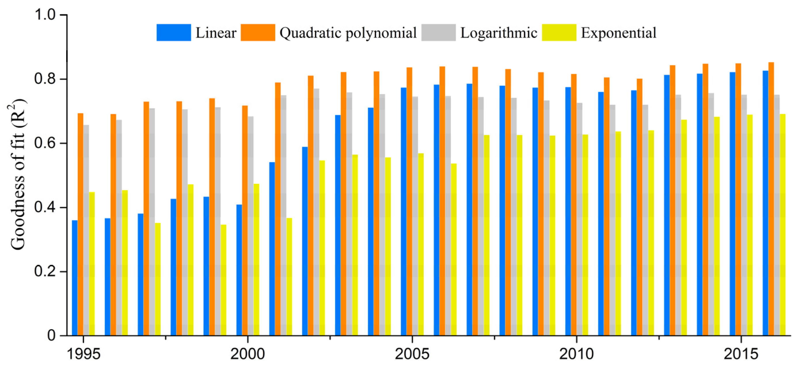
• The panel data model has proved to be feasible to estimate energy consumption at a high resolution using nighttime light data and provincial energy consumption statistics. According to the goodness of fit of the correlation (linear, quadratic polynomial, logarithmic, and exponential) between the statistical energy consumption and total nighttime light, the quadratic polynomial with the highest goodness of fit was selected to simulate energy consumption. Then, two different models, namely the quadratic polynomial model and the panel data model, were structured for energy consumption estimation, and the estimation results of these two models were assessed respectively based on the prefectural statistical data. According to the accuracy results, the panel data model performed better than the quadratic polynomial model. Additionally, from the accuracy evaluation results, our estimation results based on the panel data model are more credible compared with the existing related research.
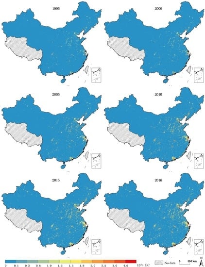
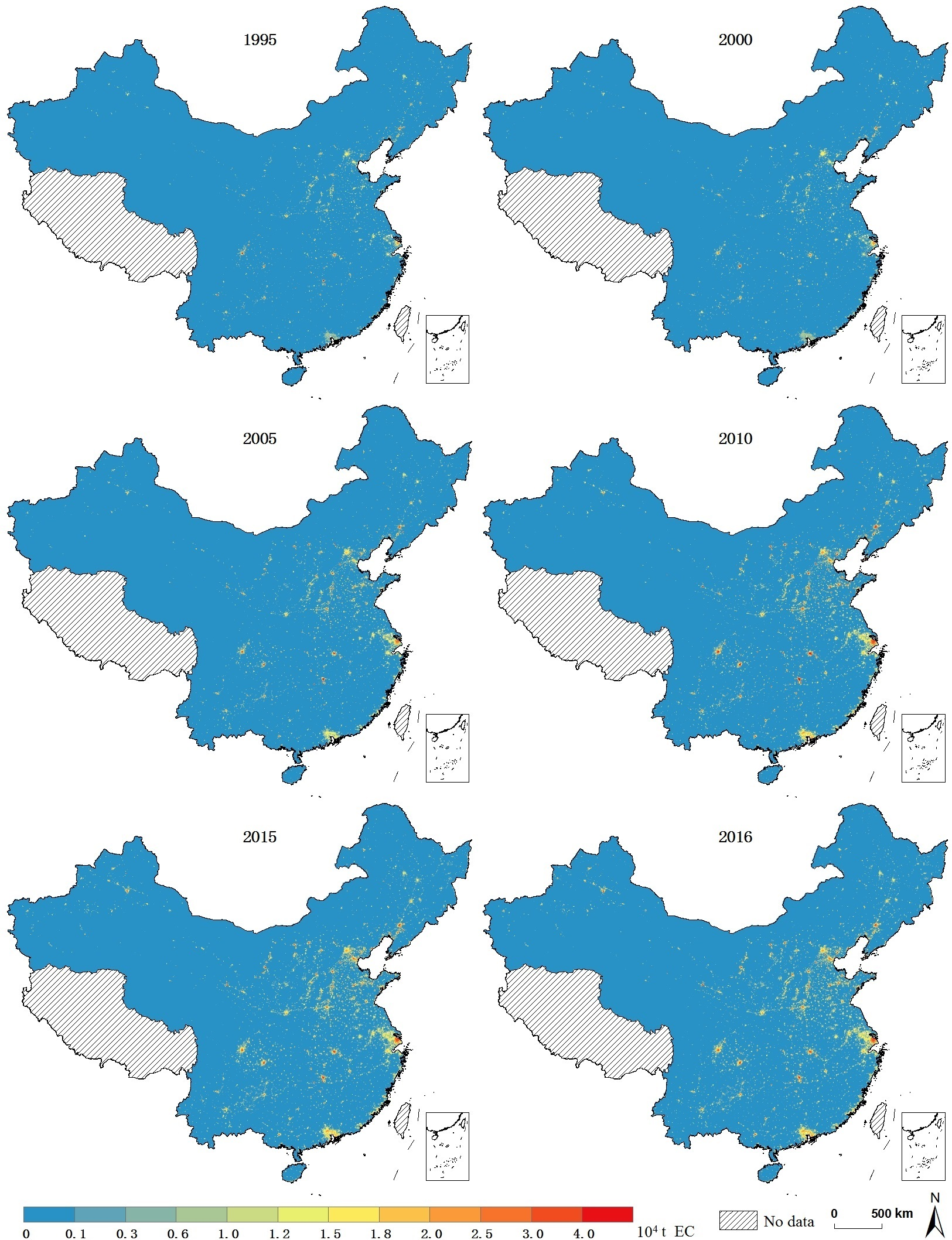
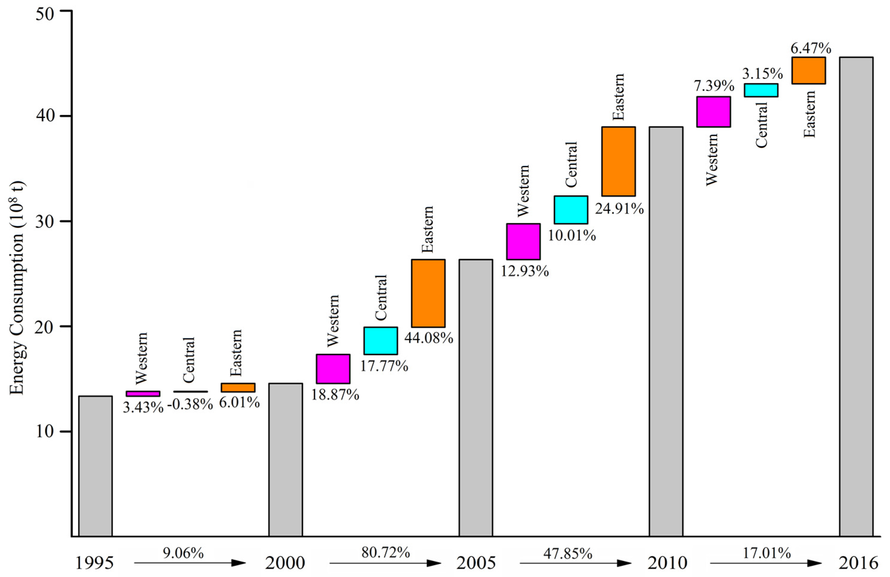
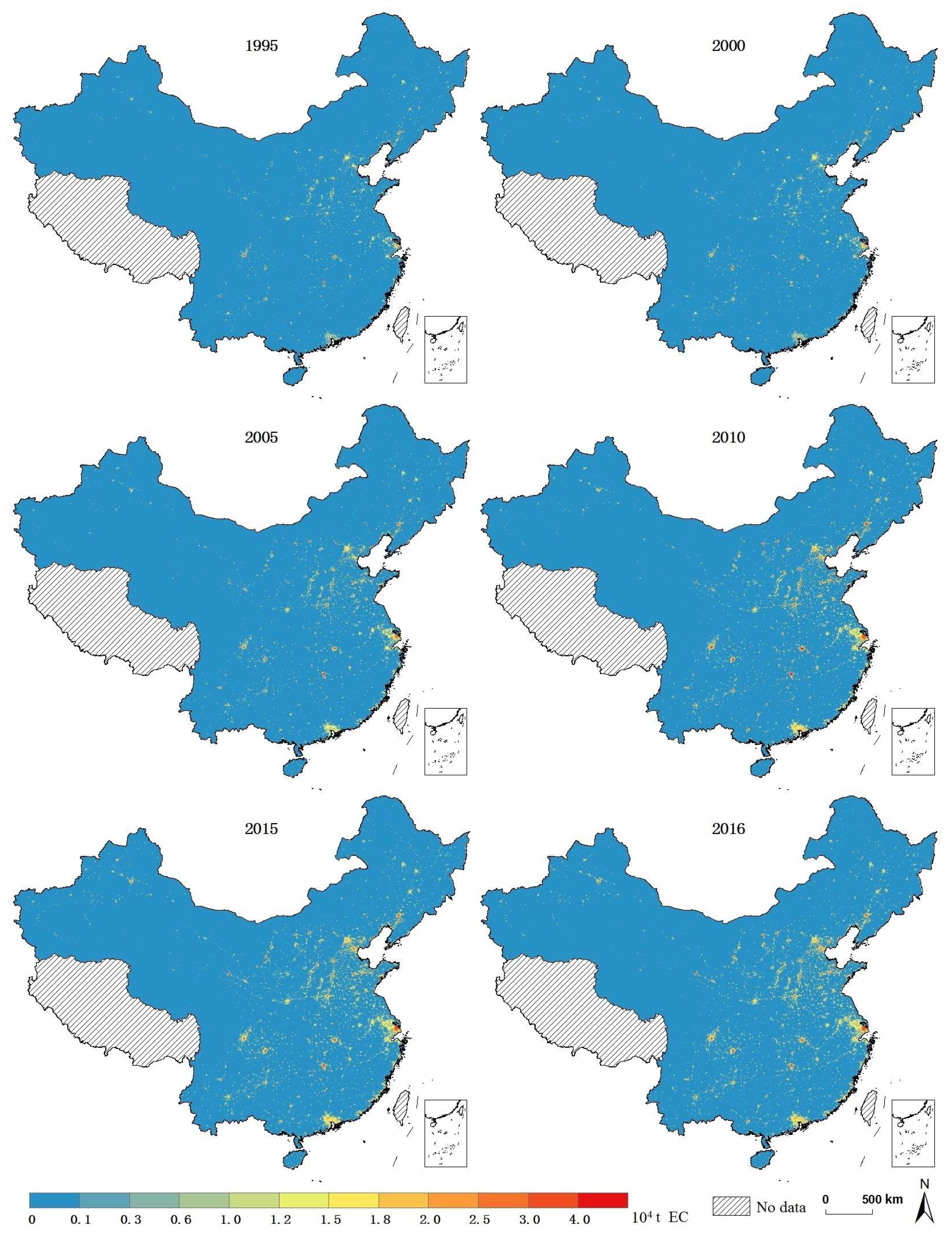
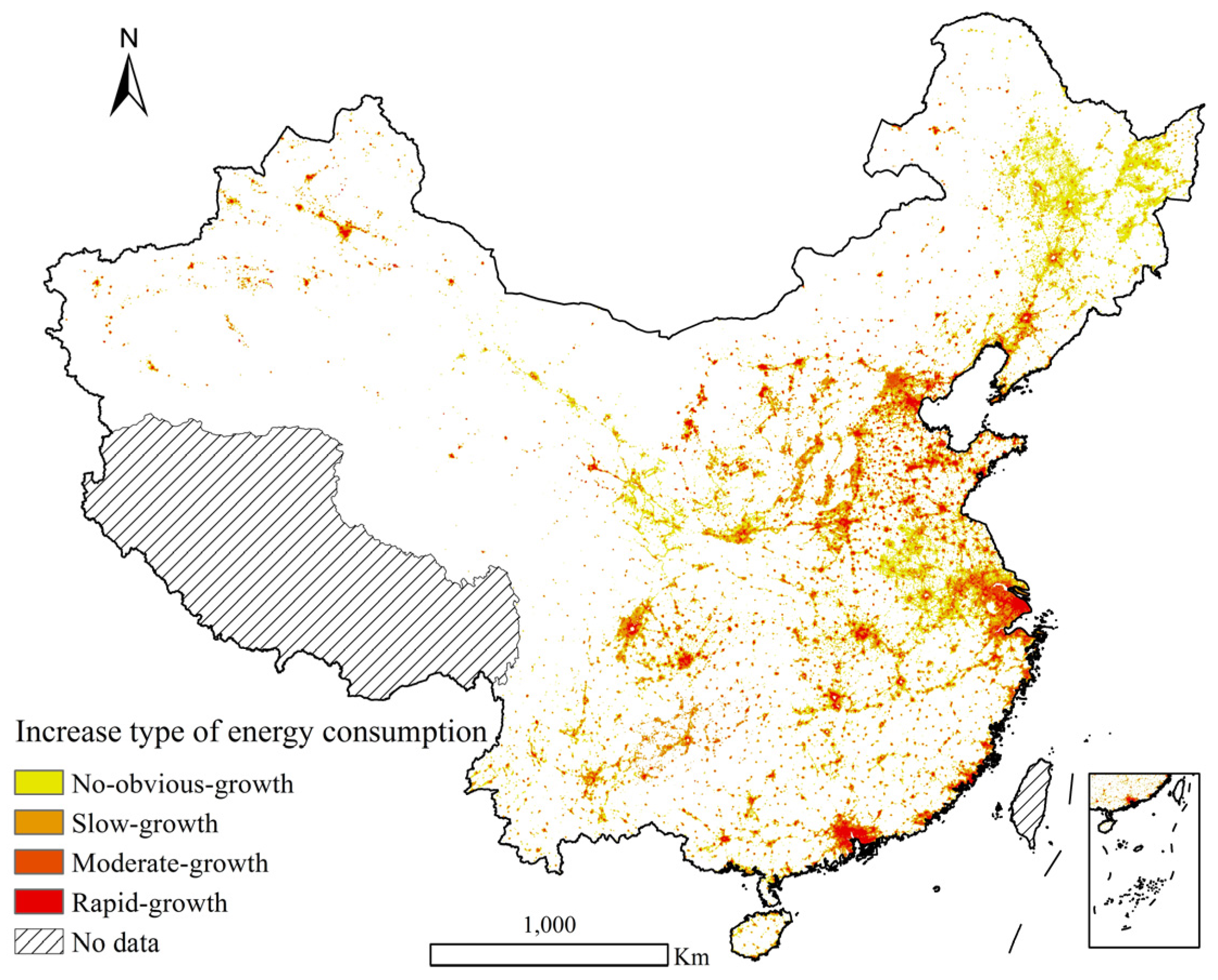
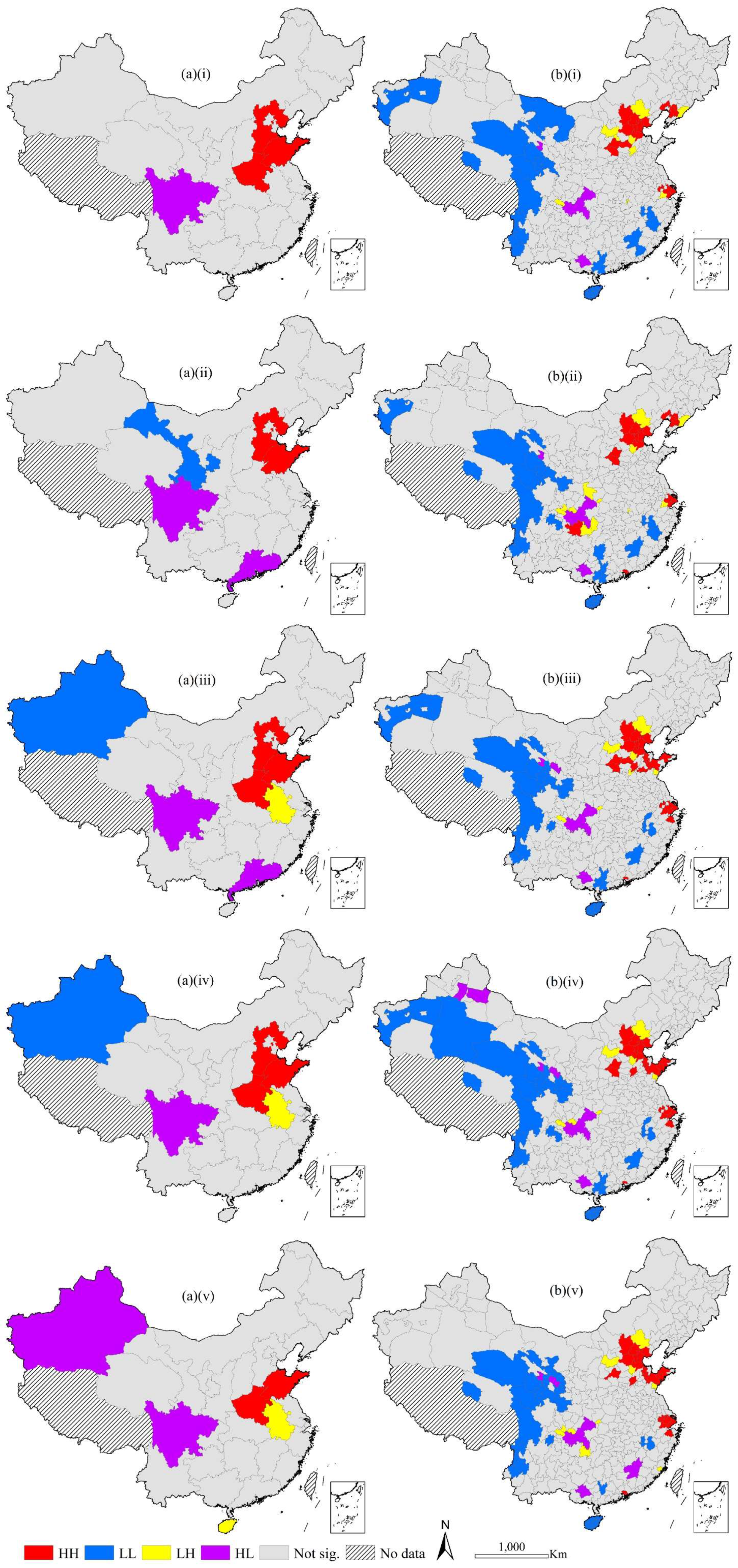
• From 1995 to 2016, the energy consumption in China significantly increased, especially in the Yangtze River Delta, the Pearl River Delta, the Beijing–Tianjin–Hebei region, eastern coastal cities, and provincial capitals, such as Chongqing, Chengdu, Wuhan, Changsha, Zhengzhou, and Shenyang. Different from the random spatial distribution pattern of energy consumption on the provincial level, the spatial distribution of energy consumption on the prefectural level has significant clustering, and its spatial agglomeration was strengthened year by year during the research period.
• The SDM model with the spatial fixed effect has proved to be more suitable to explore the impact mechanism of China’s energy consumption. Among the four socio-economic factors, industrial structure is the most important influencing factor of provincial energy intensity in China. Moreover, the changes in industrial structure and FDI can not only leave a deep influence on the local energy intensity but also affect the energy intensity of surrounding provinces.

Aiming at cutting down the national energy intensity for realizing a harmonious development of both economy and environment, three policy proposals on the basis of the spatiotemporal distribution characteristics and the influential mechanism of China’s energy consumption were put forward:

• When formulating the development policy of a regional economy, we should take into account the mutual influence of economy and industries between the adjacent regions. Considering the significant spatial spillover effect of provincial energy intensity, the construction of the economy demonstration area with the low-energy consumption industry can be conducive to reducing the energy intensity of the surrounding provinces.
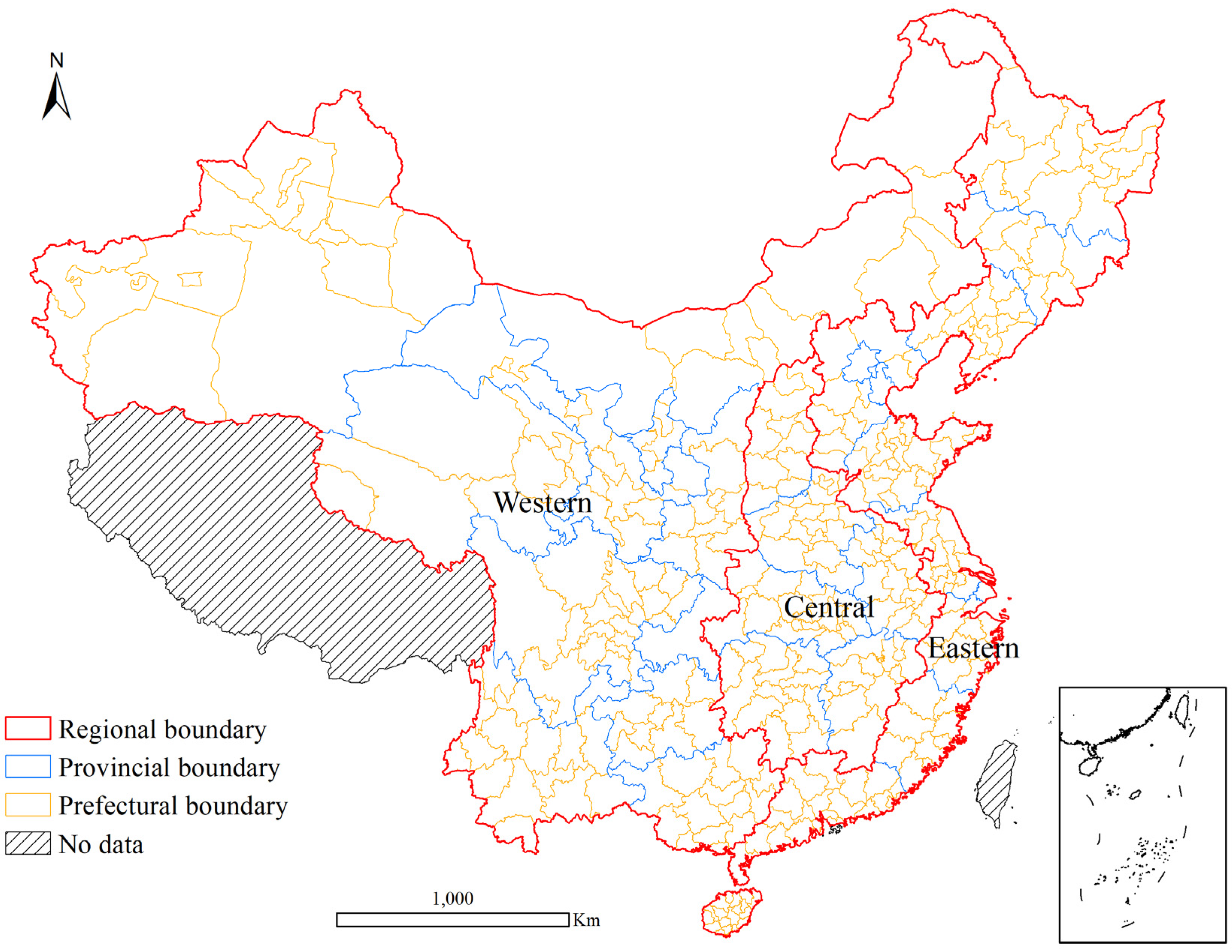
• Considering the great differences of energy intensity among regions, the Chinese government should adopt differentiated strategies for different regions. For example, for the eastern and central regions with higher levels of economic development, the reduction strategies of energy intensity should focus on adjusting and optimizing the industrial structure. That is to say, reduce the proportion of the second industry and increase the proportion of the third industry in the national economic structure.
• Governments should continue to improve the business environment and attract green foreign direct investment. Due to the advanced technology and scientific management experience, foreign-funded enterprises can play a demonstrating and promoting role in improving the production technology of the domestic enterprises and increasing the production efficiency of the whole society.

The methodology of the spatiotemporal variations in energy consumption and their influencing factors in China based on nighttime light data developed in this article can be extensively used to energy consumption spatiotemporal estimation and influencing factors analysis on the global, national, and regional levels. It can provide a quick and accurate supplement to the monitoring on continuous variations in energy consumption, with the update of NPP-VIIRS nighttime light data. This methodology can also be used as a reference for similar studies involving power consumption, CO₂ emissions, population distribution, and economic development, etc.

References

1. BP Statistical Review of World Energy. Available online: http://www.bp.com/statisticalreview (accessed on 19 December 2019).
2. Lv, Y.; Chen, W.; Cheng, J. Modelling dynamic impacts of urbanization on disaggregated energy consumption in China: A spatial Durbin modelling and decomposition approach. Energy Policy 2019, 133, 110841. [Google Scholar] [CrossRef]
3. Annual Report on China’s Energy Development. Available online: http://www.chinadaily.com.cn/ (accessed on 19 December 2019).
4. Yang, S.; Shi, L. Prediction of long-term energy consumption trends under the New National Urbanization Plan in China. J. Clean. Prod. 2017, 166, 1144–1153. [Google Scholar] [CrossRef]
5. Wu, X.F.; Chen, G.Q. Energy use by Chinese economy: A systems cross-scale input-output analysis. Energy Policy 2017, 108, 81–90. [Google Scholar] [CrossRef]
6. Lin, B.; Raza, M.Y. Analysis of energy related CO2 emissions in Pakistan. J. Clean. Prod. 2019, 219, 981–993. [Google Scholar] [CrossRef]
7. Pachauri, R.K.; Allen, M.R.; Barros, V.R.; Broome, J.; Cramer, W.; Christ, R.; Church, J.A.; Clarke, L.; Dahe, Q.; Dasgupta, P.; et al. Climate Change 2014: Synthesis Report. Contribution of Working Groups I, II and III to the Fifth Assessment Report of the Intergovernmental Panel on Climate Change; IPCC: Geneva, Switzerland, 2014. [Google Scholar]
8. He, J. What is the role of openness for China’s aggregate industrial SO2 emission? A structural analysis based on the Divisia decomposition method. Ecol. Econ. 2010, 69, 868–886. [Google Scholar] [CrossRef]
9. Wang, J.; Ma, Y.; Qiu, Y.; Liu, L.; Dong, Z. Spatially differentiated effects of socioeconomic factors on China’s NOx generation from energy consumption: Implications for mitigation policy. J. Environ. Manag. 2019, 250, 109417. [Google Scholar] [CrossRef]
10. Bilgen, S. Structure and environmental impact of global energy consumption. Renew. Sustain. Energy Rev. 2014, 38, 890–902. [Google Scholar] [CrossRef]
11. He, L.; Yin, F.; Wang, D.; Yang, X.; Xie, F. Research on the relationship between energy consumption and air quality in the Yangtze River Delta of China: An empirical analysis based on 20 sample cities. Environ. Sci. Pollut. Res. 2019, 27, 4786–4798. [Google Scholar] [CrossRef]
12. Wang, S.; Li, C.; Zhou, H. Impact of China’s economic growth and energy consumption structure on atmospheric pollutants: Based on a panel threshold model. J. Clean. Prod. 2019, 236, 117694. [Google Scholar] [CrossRef]
13. Zhang, X.; Cheng, X. Energy consumption, carbon emissions, and economic growth in China. Ecol. Econ. 2009, 68, 2706–2712. [Google Scholar] [CrossRef]
14. Wang, S.S.; Zhou, D.Q.; Zhou, P.; Wang, Q.W. CO2 emissions, energy consumption and economic growth in China: A panel data analysis. Energy Policy 2011, 39, 4870–4875. [Google Scholar] [CrossRef]
15. Arouri, M.E.H.; Ben Youssef, A.; M’Henni, H.; Rault, C. Energy consumption, economic growth and CO2 emissions in Middle East and North African countries. Energy Policy 2012, 45, 342–349. [Google Scholar] [CrossRef] [Green Version]
16. Vo, A.T.; Vo, D.H.; Le, Q.T. CO2 Emissions, Energy Consumption, and Economic Growth: New Evidence in the ASEAN Countries. J. Risk Financ. Manag. 2019, 12, 145. [Google Scholar] [CrossRef] [Green Version]
17. Nguyen, H.M.; Ngoc, B.H. Energy Consumption—Economic Growth Nexus in Vietnam: An ARDL Approach with a Structural Break. J. Asian Financ. Econ. Bus. 2020, 7, 101–110. [Google Scholar] [CrossRef]
18. de Freitas, L.C.; Kaneko, S. Decomposition of CO2 emissions change from energy consumption in Brazil: Challenges and policy implications. Energy Policy 2011, 39, 1495–1504. [Google Scholar] [CrossRef]
19. Cheng, Y.; Wang, Z.; Ye, X.; Wei, Y.D. Spatiotemporal dynamics of carbon intensity from energy consumption in China. J. Geogr. Sci. 2014, 24, 631–650. [Google Scholar] [CrossRef] [Green Version]
20. Mousavi, B.; Lopez, N.S.A.; Biona, J.B.M.; Chiu, A.S.F.; Blesl, M. Driving forces of Iran’s CO2 emissions from energy consumption: An LMDI decomposition approach. Appl. Energy 2017, 206, 804–814. [Google Scholar] [CrossRef]
21. Lv, Q.; Liu, H.; Wang, J.; Liu, H.; Shang, Y. Multiscale analysis on spatiotemporal dynamics of energy consumption CO2 emissions in China: Utilizing the integrated of DMSP-OLS and NPP-VIIRS nighttime light datasets. Sci. Total Environ. 2020, 703, 134394. [Google Scholar] [CrossRef]
22. Adua, L.; Clark, B.; York, R.; Chen, C. Modernizing our way out or digging ourselves in? Reconsidering the impacts of efficiency innovations and affluence on residential energy consumption, 2005–2015. J. Environ. Manag. 2019, 252, 109659. [Google Scholar] [CrossRef]
23. Zhang, P.; Ma, X.; She, K. A Novel Power-Driven Grey Model with Whale Optimization Algorithm and Its Application in Forecasting the Residential Energy Consumption in China. Complexity 2019, 2019, 1–22. [Google Scholar] [CrossRef]
24. Zou, B.; Luo, B. Rural household energy consumption characteristics and determinants in China. Energy 2019, 182, 814–823. [Google Scholar] [CrossRef]
25. Tian, S.; Chang, S. An agent-based model of household energy consumption. J. Clean. Prod. 2020, 242, 118378. [Google Scholar] [CrossRef]
26. Liu, X.; Ou, J.; Wang, S.; Li, X.; Yan, Y.; Jiao, L.; Liu, Y. Estimating spatiotemporal variations of city-level energy-related CO2 emissions: An improved disaggregating model based on vegetation adjusted nighttime light data. J. Clean. Prod. 2018, 177, 101–114. [Google Scholar] [CrossRef]
27. Zhang, Q.; Seto, K.C. Mapping urbanization dynamics at regional and global scales using multi-temporal DMSP/OLS nighttime light data. Remote Sens. Environ. 2011, 115, 2320–2329. [Google Scholar] [CrossRef]
28. Yu, B.; Yu, B.; Shu, S.; Liu, H.; Song, W.; Wu, J.; Wang, L.; Chen, Z. Object-based spatial cluster analysis of urban landscape pattern using nighttime light satellite images: A case study of China. Int. J. Geogr. Inf. Sci. 2014, 28, 2328–2355. [Google Scholar] [CrossRef]
29. Li, Q.; Lu, L.; Weng, Q.; Xie, Y.; Guo, H. Monitoring Urban Dynamics in the Southeast, U.S.A. Using Time-Series DMSP/OLS Nightlight Imagery. Remote Sens. 2016, 8, 578. [Google Scholar] [CrossRef] [Green Version]
30. Min, Z.; Cheng, W.; Zhou, C.; Li, M.; Huang, K.; Nan, W. Assessing Spatiotemporal Characteristics of Urbanization Dynamics in Southeast Asia Using Time Series of DMSP/OLS Nighttime Light Data. Remote Sens. 2018, 10, 47. [Google Scholar]
31. Zhuo, L.; Ichinose, T.; Zheng, J.; Chen, J.; Shi, P.J.; Li, X. Modelling the population density of China at the pixel level based on DMSP/OLS non-radiance-calibrated night-time light images. Int. J. Remote Sens. 2009, 30, 1003–1018. [Google Scholar] [CrossRef]
32. Tripathi, B.R.; Tiwari, V.; Pandey, V.; Elvidge, C.; Rawat, J.S.; Sharma, M.P.; Pravasi, R.; Kumar, P. Estimation of Urban Population Dynamics using DMSP-OLS Night-time Lights Time Series Sensors Data. IEEE Sens. J. 2017, 17, 1013–1020. [Google Scholar] [CrossRef]
33. Tan, M.; Li, X.; Li, S.; Xin, L.; Wang, X.; Li, Q.; Li, W.; Li, Y.; Xiang, W. Modeling population density based on nighttime light images and land use data in China. Appl. Geogr. 2018, 90, 239–247. [Google Scholar] [CrossRef]
34. Li, X.; Xu, H.; Chen, X.; Li, C. Potential of NPP-VIIRS Nighttime Light Imagery for Modeling the Regional Economy of China. Remote Sens. 2013, 5, 3057–3081. [Google Scholar] [CrossRef] [Green Version]
35. Keola, S.; Andersson, M.; Hall, O. Monitoring Economic Development from Space: Using Nighttime Light and Land Cover Data to Measure Economic Growth. World Dev. 2015, 66, 322–334. [Google Scholar] [CrossRef]
36. Meng, L.; Graus, W.; Worrell, E.; Bo, H. Estimating CO2 (carbon dioxide) emissions at urban scales by DMSP/OLS (Defense Meteorological Satellite Program’s Operational Linescan System) nighttime light imagery: Methodological challenges and a case study for China. Energy 2014, 71, 468–478. [Google Scholar] [CrossRef]
37. Ou, J.; Liu, X.; Li, X.; Shi, X. Mapping Global Fossil Fuel Combustion CO2 Emissions at High Resolution by Integrating Nightlight, Population Density, and Traffic Network Data. IEEE J. Sel. Top. Appl. Earth Obs. Remote Sens. 2016, 9, 1674–1684. [Google Scholar] [CrossRef]
38. Shi, K.; Yu, B.; Zhou, Y.; Chen, Y.; Yang, C.; Chen, Z.; Wu, J. Spatiotemporal variations of CO2 emissions and their impact factors in China: A comparative analysis between the provincial and prefectural levels. Appl. Energy 2019, 233, 170–181. [Google Scholar] [CrossRef]
39. Elvidge, C.D.; Baugh, K.E.; Kihn, E.A.; Kroehl, H.W.; Davis, E.R.; Davis, C.W. Relation between satellite observed visible-near infrared emissions, population, economic activity and electric power consumption. Int. J. Remote Sens. 1997, 18, 1373–1379. [Google Scholar] [CrossRef]
40. Amaral, S.; Câmara, G.; Monteiro, A.M.V.; Quintanilha, J.A.; Elvidge, C.D. Estimating population and energy consumption in Brazilian Amazonia using DMSP night-time satellite data. Comput. Environ. Urban Syst. 2005, 29, 179–195. [Google Scholar] [CrossRef]
41. Chand, T.R.K.; Badarinath, K.V.S.; Elvidge, C.D.; Tuttle, B.T. Spatial characterization of electrical power consumption patterns over India using temporal DMSP-OLS night-time satellite data. Int. J. Remote Sens. 2009, 30, 647–661. [Google Scholar] [CrossRef]
42. He, C.; Ma, Q.; Li, T.; Yang, Y.; Liu, Z. Spatiotemporal dynamics of electric power consumption in Chinese Mainland from 1995 to 2008 modeled using DMSP/OLS stable nighttime lights data. J. Geogr. Sci. 2012, 22, 125–136. [Google Scholar] [CrossRef]
43. Letu, H.; Hara, M.; Tana, G.; Bao, Y.; Nishio, F. Generating the Nighttime Light of the Human Settlements by Identifying Periodic Components from DMSP/OLS Satellite Imagery. Environ. Sci. Technol. 2015, 49, 10503–10509. [Google Scholar] [CrossRef]
44. Shi, K.; Chen, Y.; Yu, B.; Xu, T.; Yang, C.; Li, L.; Huang, C.; Chen, Z.; Liu, R.; Wu, J. Detecting spatiotemporal dynamics of global electric power consumption using DMSP-OLS nighttime stable light data. Appl. Energy 2016, 184, 450–463. [Google Scholar] [CrossRef]
45. Xie, Y.; Weng, Q. World energy consumption pattern as revealed by DMSP-OLS nighttime light imagery. Gisci. Remote Sens. 2016, 53, 265–282. [Google Scholar] [CrossRef]
46. Wu, J.; Niu, Y.; Peng, J.; Wang, Z.; Huang, X. Research on energy consumption dynamic among prefecture-level cities in China based on DMSP/OLS Nighttime Light. Geogr. Res. 2014, 33, 625–634. [Google Scholar] [CrossRef]
47. Wu, L.; Kaneko, S.; Matsuoka, S. Driving forces behind the stagnancy of China’s energy-related CO2 emissions from 1996 to 1999: The relative importance of structural change, intensity change and scale change. Energy Policy 2005, 33, 319–335. [Google Scholar] [CrossRef]
48. Yu, Y.; Kong, Q. Analysis on the influencing factors of carbon emissions from energy consumption in China based on LMDI method. Nat. Hazards 2017, 88, 1691–1707. [Google Scholar] [CrossRef]
49. Tian, X.; Chang, M.; Tanikawa, H.; Shi, F.; Imura, H. Regional Disparity in Carbon Dioxide Emissions: Assessing Sectoral Impacts on the Carbon Dioxide Emissions Structure among Regions of Mainland China. J. Ind. Ecol. 2012, 16, 612–622. [Google Scholar] [CrossRef]
50. Wang, C.; Wang, F.; Zhang, X.; Zhang, H. Influencing mechanism of energy-related carbon emissions in Xinjiang based on the input-output and structural decomposition analysis. J. Geogr. Sci. 2017, 27, 365–384. [Google Scholar] [CrossRef] [Green Version]
51. Lin, B.; Du, K. Decomposing energy intensity change: A combination of index decomposition analysis and production-theoretical decomposition analysis. Appl. Energy 2014, 129, 158–165. [Google Scholar] [CrossRef]
52. Liu, Q.; Wang, S.; Zhang, W.; Zhan, D.; Li, J. Does foreign direct investment affect environmental pollution in China’s cities? A spatial econometric perspective. Sci. Total Environ. 2018, 613, 521–529. [Google Scholar] [CrossRef]
53. Kang, Y.; Zhao, T.; Wu, P. Impacts of energy-related CO2 emissions in China: A spatial panel data technique. Nat. Hazards 2016, 81, 405–421. [Google Scholar] [CrossRef]
54. Yu, H. The influential factors of China’s regional energy intensity and its spatial linkages: 1988–2007. Energy Policy 2012, 45, 583–593. [Google Scholar] [CrossRef]
55. Zhao, X.; Lu, F. Spatial distribution characteristics and convergence of China’s regional energy intensity: An industrial transfer perspective. J. Clean. Prod. 2019, 233, 903–917. [Google Scholar] [CrossRef]
56. Baugh, K.; Hsu, F.; Elvidge, C.D.; Zhizhin, M. Nighttime Lights Compositing Using the VIIRS Day-Night Band: Preliminary Results. Proc. Asia Pac. Adv. Netw. 2013, 35, 70–86. [Google Scholar] [CrossRef] [Green Version]
57. Elvidge, C.D.; Baugh, K.E.; Zhizhin, M.; Hsu, F. Why VIIRS data are superior to DMSP for mapping nighttime lights. Proc. Asia Pac. Adv. Netw. 2013, 35, 62–69. [Google Scholar] [CrossRef] [Green Version]
58. Zhao, J.; Ji, G.; Yue, Y.; Lai, Z.; Chen, Y.; Yang, D.; Yang, X.; Wang, Z. Spatio-temporal dynamics of urban residential CO2 emissions and their driving forces in China using the integrated two nighttime light datasets. Appl. Energy 2019, 235, 612–624. [Google Scholar] [CrossRef]
59. Bai, C. Study on spatial and temporal dynamic evolution of energy consumption in prefecture-level city of China based on multi-source remote sensing data. Master’s Thesis, Nanchang University, Nanchang, China, 28 May 2016. [Google Scholar]
60. Shi, K.; Chen, Y.; Yu, B.; Xu, T.; Chen, Z.; Liu, R.; Li, L.; Wu, J. Modeling spatiotemporal CO2 (carbon dioxide) emission dynamics in China from DMSP-OLS nighttime stable light data using panel data analysis. Appl. Energy 2016, 168, 523–533. [Google Scholar] [CrossRef]
61. Xie, H.; Zou, J.; Peng, X. Spatial-temporal Difference Analysis of Cultivated Land Use Intensity Based on Emergy in Poyang Lake Eco-economic Zone. Acta Geogr. Sin. 2012, 67, 889–902. [Google Scholar]
62. Zhang, Y.; Xu, J.; Zhuang, P. The Spatial Relationship of Tourist Distribution in Chinese Cities. Tour. Geogr. 2011, 13, 75–90. [Google Scholar] [CrossRef]
63. Adom, P.K. Asymmetric impacts of the determinants of energy intensity in Nigeria. Energy Econ. 2015, 49, 570–580. [Google Scholar] [CrossRef]
64. Yang, G.; Li, W.; Wang, J.; Zhang, D. A comparative study on the influential factors of China’s provincial energy intensity. Energy Policy 2016, 88, 74–85. [Google Scholar] [CrossRef]
65. Farajzadeh, Z.; Nematollahi, M.A. Energy intensity and its components in Iran: Determinants and trends. Energy Econ. 2018, 73, 161–177. [Google Scholar] [CrossRef]
66. Mahmood, T.; Ahmad, E. The relationship of energy intensity with economic growth: Evidence for European economies. Energy Strategy Rev. 2018, 20, 90–98. [Google Scholar] [CrossRef]
67. Rajbhandari, A.; Zhang, F. Does energy efficiency promote economic growth? Evidence from a multicountry and multisectoral panel dataset. Energy Econ. 2018, 69, 128–139. [Google Scholar] [CrossRef] [Green Version]
68. LeSage, J.; Pace, R.K. Introduction to Spatial Econometrics; CRC Press: Boca Raton, FL, USA, 2009. [Google Scholar]
Figure 1. Spatial distribution of the study area.
Remotesensing 12 01151 g001
Figure 2. Goodness of fit of energy consumption and the total digital number values (TDN) of nighttime light data in China.
Remotesensing 12 01151 g002
Figure 3. Changes in energy consumption from three Chinese regions for 1995–2016.
Remotesensing 12 01151 g003
Figure 4. Distribution map of energy consumption in China based on the panel data model for 1995–2016.
Remotesensing 12 01151 g004
Figure 5. Four classes of the increments of energy consumption in China for 1995–2016 (Note: the non-positive growth was masked).
Remotesensing 12 01151 g005
Figure 6. (a) Areal proportion of each type of energy consumption in China. (b) Areal proportion of each type in the three regions.
Remotesensing 12 01151 g006
Figure 7. Spatial clusters for energy consumption on the (a) provincial level and the (b) prefectural level in (i) 1995, (ii) 2000, (iii) 2005, (iv) 2010, and (v) 2016.
Remotesensing 12 01151 g007