Article

VIIRS Day/Night Band—Correcting Striping and Nonuniformity over a Very Large Dynamic Range

1
Renaissance Man Engineering, Glendale, CA 91202, USA
2
Cooperative Institute for Research in the Atmosphere, Colorado State University, Fort Collins, CO 80523, USA
*
Author to whom correspondence should be addressed.
J. Imaging 2016, 2(1), 9; https://doi.org/10.3390/jimaging2010009
Submission received: 1 December 2015 / Revised: 26 January 2016 / Accepted: 26 February 2016 / Published: 14 March 2016
(This article belongs to the Special Issue Big Visual Data Processing and Analytics)

Abstract

:
The Suomi National Polar-orbiting (NPP) Visible Infrared Imaging Radiometer Suite (VIIRS) Day-Night Band (DNB) measures visible and near-infrared light extending over seven orders of magnitude of dynamic range. This makes radiometric calibration difficult. We have observed that DNB imagery has striping, banding and other nonuniformities—day or night. We identified the causes as stray light, nonlinearity, detector crosstalk, hysteresis and mirror-side variation. We found that these affect both Earth-view and calibration signals. These present an obstacle to interpretation by users of DNB products. Because of the nonlinearity we chose the histogram matching destriping technique which we found is successful for daytime, twilight and nighttime scenes. Because of the very large dynamic range of the DNB, we needed to add special processes to the histogram matching to destripe all scenes, especially imagery in the twilight regions where scene illumination changes rapidly over short distances. We show that destriping aids image analysts, and makes it possible for advanced automated cloud typing algorithms. Manual or automatic identification of other features, including polar ice and gravity waves in the upper atmosphere are also discussed. In consideration of the large volume of data produced 24 h a day by the VIIRS DNB, we present methods for reducing processing time.

Graphical Abstract

1. Introduction

The Day/Night Band (DNB) on the Visible Infrared Imaging Radiometer Suite (VIIRS) is part of Suomi National Polar-orbiting Partnership (S-NPP) satellite launched on 28 October 2011. The DNB is a panchromatic visible to near infrared band designed to detect radiance from the brightest daytime scenes down to very dim nighttime scenes illuminated by quarter moon. Its dynamic range comprises over seven orders of magnitude. The sensitivity of the DNB to very low radiance levels requires cross-calibration over three gain stages, and this makes maintaining uniformity on DNB much more difficult than for other bands on VIIRS. Other than uniformity, based on post-launch characterization, VIIRS DNB has met its radiometric and spatial resolution requirements [1].
Since the launch of S-NPP, the low-light detection capabilities of VIIRS DNB have opened new areas of research including the detection of nightglow and features illuminated by nightglow [2,3] and development of long-term climate data records. Because of these new areas, the required quality of DNB data has been pushed beyond the originally intended design limits. Therefore, striping and other nonuniformities have become limiting factors in these new areas of research [4]. Reducing these artifacts would extend the usefulness of the DNB in these new areas.
Striping is usually caused by detector-to-detector response that is not corrected by calibration. Banding occurs when there are differences in response for all detectors among scans, and for the DNB in particular, between aggregation zones. Figure 1 shows an example of the DNB striping and banding problems. This is a nighttime image from 23 October 2015 when the moon is waxing with phase about half way between the first quarter and full. It is of Hurricane Patricia at about the time it became the strongest Pacific hurricane on record. Unfortunately, in this image the eye of the hurricane is near the edge of the VIIRS swath where the DNB striping is typically the most extreme. At night weather analysts mostly depend on thermal-emissive infrared imagery to evaluate hurricanes and storms, but these images lack the texture and fine structure that Reflective Solar Band (RSB) images provide particularly with regard to low cloud fields which often provide insight to the structure of low-level circulation. The VIIRS DNB is one of the only instruments for which such nocturnal information is available, and so provides a very important insight when available. This example illustrates the magnitude of striping due to gain errors. Note the vertical banding just to the right of the hurricane’s eye. This feature is prominent in most nighttime DNB imagery, and correcting this will be discussed later in this paper.
This paper considers striping and other nonuniformities in the VIIRS DNB imagery on S-NPP. It considers the current methods of calibration, as well as recent changes, and diagnoses the root cause of residual striping that remains after calibration. It also presents a methodology for eliminating most nonuniformity for daytime, twilight and nighttime. We previously published results demonstrating destriping for imagery using the Moment Matching (MM) method, but this correction was limited to nighttime scenes with limited dynamic range [5]. Here we demonstrate for the first time destriping over the entire dynamic range of the DNB using the Histogram Matching Method (HMM). Examples of HMM applied to a variety of scenes and degrees of striping severity are shown. Because of the huge dynamic range of the DNB, there are special ensemble filtering processes required to enhance the standard procedures used for HMM that will be presented in this paper.

1.1. VIIRS Design

The VIIRS design was primarily based on the MODIS instrument heritage. However, unlike MODIS, VIIRS also has the DNB, which has more stringent stray light exclusion requirements. Thus, VIIRS was specifically designed to suppress stray light [6]. The first optical element in the MODIS optical path is a scan mirror used to produce its cross-track scanning. VIIRS instead uses an afocal, three-mirror anistigmat telescope, where the entire telescope assembly rotates in order to produce cross-track scanning. One reason the rotating telescope design was chosen rather than a scan-mirror was to suppress stray light. This is because the primary mirror in the telescope is recessed deeper inside the scan cavity.
As the telescope rotates it takes a view of the three calibration (cal) sectors: the Space View (SV) that points out to space just above the mesospheric limb, and occurs just before the start of the Earth-view; the Black Body (BB) view that occurs after the telescope sweeps across the Earth and is inside the instrument; and the Solar Diffuser (SD) that is illuminated by the sun through a solar attenuation screen for during a period of about 2 to 3 min per orbit when the solar geometry is right [7]. A rotating mirror relays light from the telescope to the detectors, and since it rotates at half the rate of the telescope, it is called the Half-Angle Mirror (HAM).
The DNB has a wide spectral bandpass, nominally between 500 and 900 nm. It is capable of a dynamic range in radiance of about eight orders of magnitude at nadir and seven orders of magnitude at the edges of its 3000 km wide swath. It achieves this dynamic range via a charge-coupled device focal plane array that is sectioned into four stages, where each stage essentially functions as a separate imager even though they all reside on the same detector array. The array has much higher detector resolution than what is required for the DNB’s 750 m pixel footprint, but it combines detector signals electronically in the read-out circuit, aggregating them as a function of scan position. Using variable aggregation over 32 symmetric zones about nadir, it compensates for perspective and foreshortening in a way that results in an almost constant 750 m horizontal ground resolution [8].
The four stages for the DNB are the Low-Gain Stage (LGS), Mid-Gain Stage (MGS) and two redundant High-Gain Stages (HGS). The LGS is used for daytime scenes, the MGS for twilight scenes near the Earth’s terminator, and the HGS for late twilight and nighttime scenes. Because of the complexity of the DNB circuitry it is important here to define some terms. The detector array actually has hundreds of detectors in each dimension that are aggregated into 16 virtual along-track detectors. Because only the aggregated output of these many detectors is transmitted to the ground, we will always refer to the virtual detectors as “detectors.” When we do refer to the actual preaggregated detectors, we will use the word “subpixels.” In this paper three terms are used to describe detector aggregation—aggregation mode, aggregation zone and aggregation sequence number. The terms are defined here in the way that they are usually used on the VIIRS program. “Aggregation zone” is used when referring to a specific area of the swath in the cross-track direction relative to nadir. “Aggregation mode” refers to the specific method of aggregation, that is, the number of subpixels that are aggregated in each dimension in forming a single DNB pixel. “Aggregation sequence number” refers to the aggregation mode numbering specifically in relation to the order that the aggregation modes are cycled through in the cal sector data. Therefore, this term will not be used when referring to data in the Earth-view. The aggregation zones are numbered symmetrically about nadir, with Aggregation Mode 1 at nadir and Aggregation Mode 32 at edge of scan. This is opposite the Aggregation Sequence Number, so that Aggregation Mode 1 is Aggregation Sequence Number 32 and vice versa. There are also four additional aggregation modes that are not used in any of the aggregation zones in the Earth-view. These are sometimes referred to as super-aggregation modes because they aggregate many pixels. There are 64 aggregation zones in the Earth-view and 36 aggregation modes. In the cal sector the aggregation sequence numbers are repeated every 72 scans with each aggregation mode being used for two scans of cal sector data in order to allow both HAM sides to be calibrated.

1.2. On-Orbit DNB Calibration Process

Since the DNB calibration process is related to the root causes of striping, we describe it in detail here. Data that are collected by VIIRS on-orbit and processed on the ground to produce radiometrically calibrated and geolocated radiances are called the Sensor Data Record (SDR), or alternately the Level 1 product. The SDR is produced by the Interface Data Processing Segment (IDPS) that is part of the Common Ground System developed under contract by Raytheon for NOAA [9]. The DNB is just one of 22 VIIRS bands, but because of the complexity of the DNB electronics described above, the DNB calibration process is by far the most complex. In addition to the IDPS DNB SDR, NASA Land Science Investigator-led Processing System (Land SIPS) in coordination with the Suomi-NPP VIIRS Calibration Support Team (VCST) produces a DNB Level 1 product using a similar calibration process. Land-SIPS system is maintained separately from IDPS in order to develop new algorithms and to support reprocessing of data [10]. There have been some major changes to the DNB calibration, and both the original process and the recent changes are described here since both are relevant and depend on when the SDR used for imagery is created.

1.2.1. Original DNB Calibration Process

The original process for offset was devised based on pre-launch testing of the instrument and is described in full in the VIIRS SDR Calibration Algorithm Theoretical Basis Document [11]. In these tests it was found that the offsets observed in the space view were not consistent with the offsets observed in the Earth-view for any of the gain stages, and in addition, the Earth-view has a fixed-pattern noise that is not constant in the scan direction, even within a single aggregation zone. The possible reason for this discrepancy will be discussed later in the section Causes of DNB non-uniformity. Because of these issues, an alternative offset measurement was needed and it was decided that dark Earth scenes over the Pacific would be used to determine an offset for each of the 4064 pixels within a scan. Since the MGS and LGS are normally not transmitted at night, it was decided that once every lunar month around the time of new moon a special process would be run that transmits the MGS and LGS in addition to the HGS data. Any bright lights from islands or ships are then filtered out as outliers and the remaining data are averaged to produce an offset table for every detector, HAM side, gain state and in-scan pixel. Other statistical tests are also done to determine whether the data has the characteristics of dark noise [11,12].
The gain calibration process for the LGS is similar to the other Reflective Solar Bands (RSB) on VIIRS. Data are collected for the DNB as it views the three cal sectors. The mean counts of the SV sector is subtracted from the SD view, and using knowledge of the SD reflectance, attenuation screen transmittance and solar geometry, a reference radiance is calculated to determine the gain in radiance per digital count. For the DNB, however, there is a complication in that it has 36 Aggregation Sequence Numbers (ASN), 32 of which are used in the Earth-view. To accommodate this the DNB cal sectors undergo a 72 scan cycle with a scan for each HAM side and ASN combination. [13].
Because the solar-illuminated SD radiance saturates the MGS and the HGS, these require a cross-calibration process. As with the offset calibration, the special mode that sends MGS and LGS is enabled, but for cross-calibration this needs to be done around the terminator region as the Earth scene transitions from night to day or day to night. It can be performed at any time during the lunar month, but because the SD is illuminated by the sun only during the night-to-day transition, this process is always performed only during the day-to-night transition, so as not to interfere with transmission of SD and SV cal sector data used for RSB gain calibration. The data simultaneously collected for HGS, MSG and LGS in the Earth-view are used to determine gain ratios between these stages. LGS gains from the SD view along with the gain ratios between each of the stages are then used to construct calibration gain tables for all the stages, ASNs and mirror side combinations [12,13].

1.2.2. DNB RSB Automatic Calibration Process

The VIIRS thermal emissive bands have always been calibrated by performing offset and gain corrections on a per-scan basis, therefore making the process completely automatic. From the beginning it was hoped that RSB calibration could eventually be automated in the same way [14], but the once-per-orbit SD view complicated gain calibration. However, fully-automated RSB calibration has recently been implemented as part of IDPS and is referred to as the RSB Automated Calibration (RSBAutoCal). For the other RSB bands, the RSBAutoCal process is relatively straightforward. The per-orbit SD events used to compute time dependent, per-detector gains are temporally filtered to produce smoothed gain corrections [15].
For the DNB the monthly updates of both the gains and the offsets have presented an almost insurmountable obstacle to automate. Nevertheless, much work has been done to achieve that goal, and the development of that process is summarized here. The use of cal sector data is key to achieving an automated calibration process. Shortly after the DNB became functional in January 2012, the VIIRS SDR Calibration/Validation (Cal/Val) Team began analyzing the cal sector data. All the cal sectors were found to be contaminated with stray light. However, during the periods when the satellite went into the Earth’s shadow, there was no stray light signal, and it was suggested that averages of the data from these periods could be used to determine offset [5,16]. This has become the basis for automated DNB offset correction. Still, the absolute offset could not be determined because of differences between the Earth-view and the cal sector, but a pitch maneuver was performed which filled the entire Earth-view sector with a view of deep space. This deep-space view has become the offset reference for the Earth-view, and the changes to offsets from the cal sector data are taken with respect to this [17,18].
The SDR Cal/Val Team also noticed during the daytime portions of the orbit that the SD cal sector signal was about two orders of magnitude higher than either the SV or BB signals. Since during the day the attenuation screen is not exposed to any direct sunlight, it was hypothesized that this strong signal was due to Earthshine (solar reflection off the Earth) coming through the attenuation screen and illuminating the SD. Looking for a technique to provide gain ratios using only the cal sector data, it was suggested that this daytime SD signal could be used for LGS-to-MGS cross-calibration and possibly MGS-to-HGS cross-calibration as well [5,19]. Concerns were raised, however, about whether sneak-path stray light might be contaminating the MGS-to-HGS gain ratios [20].
These ideas were incorporated into the operational VIIRS calibration algorithm at IDPS in December 2013 [15], but operationally it was placed in “manual mode” (as described in the previous section) until it could be fully tested off-line. In August 2015 the VIIRS RSBAutoCal was placed in automatic calibration mode for all bands except the DNB [20]. At the time of this writing, the RSBAutoCal has not yet been put into automatic mode for most of the DNB calibration, so its effects are not seen in any of the images shown here. Nevertheless, the process will be discussed here with considerations of how it would affect nonuniformity in the DNB.
The RSBAutoCal algorithm takes the gain ratio process a step further by providing the option of using not only the SD sector data, but also the BB and SV data to produce gain ratios for cross-calibration [21]. Both the BB and SV are predominantly stray light [5,15,22], so this method is based on the assumption that stray light illuminates the HGA, HGB, MGS and LGS sections of the CCD focal plane array equally. This assumption will be discussed later in the paper.
The NASA VCST has also incorporated DNB calibration algorithms similar to the RSBAutoCal [17]. An improvement that is included in the Land SIPS version is filtering out lunar stray light contamination from the offset data, after they found that it created a small bias when the moon is more than half full [17]. However, because of concerns regarding stray light, the Land SIPS version of automatic calibration no longer computes the gain ratios using the SV or BB signals [10].

2. Materials and Methods

All of the results in this paper are the product of computer processing. Here we describe the source of data, the hardware and the software, as well as our methodology.

2.1. Source of Data

The data used in this study was obtained from the Comprehensive Large Array-data Stewardship System (CLASS), an electronic library of NOAA environmental data that is available on-line [23]. For this study we used three types of datasets downloaded from CLASS: VIIRS Day Night Band SDR; VIIRS Day Night Band SDR Ellipsoid Geolocation; and VIIRS on-board calibrator data. The on-board calibrator data product is currently a restricted product, and if readers want access, they need to request permission by email at [email protected]. All images presented here are from the DNB SDR produced by the IDPS system. S-NPP datasets from CLASS are in the Hierarchal Data Format, version 5 (HDF5). For readers who wish to review the actual software used by IDPS, it is available to external organizations through the NOAA Community Satellite Processing Package [24], which supports the Direct Broadcast meteorological and environmental satellite community through the packaging and distribution of open source science software [25].

2.2. Hardware

All processing presented in this paper was performed on a Hewitt Packard Desktop computer with an Intel® Core™ i7-3770 CPU running at 3.7 GHz. The operating system was both Windows 8.1 and Windows 10. The software has also been tested on the hardware at Colorado State Univ., Fort Collins Cooperative Institute for Research in the Atmosphere.

2.3. Software Language and Libraries

All software was written in 64 bit Python 3.3 (3.3.2.1) with Numpy and Scipy libraries included. The plots were produced using Matplotlib 1.3.0. The software used in this study is copyrighted by Renaissance Man Engineering, but it can be made available to users for testing purposes upon request of the first author.

2.4. Histogram Matching Method Destriping Algorithm Description

We have tested three techniques for removing striping, and have presented some of these results previously [5]. These techniques are:
  • Offset correction for night scenes similar to what is described in the On-Orbit DNB Calibration section above.
  • Gain correction for moonlit scenes using the Moment Matching (MM) technique.
  • Complete correction over the entire dynamic range using the Histogram Matching Method (HMM).
Several other destriping techniques have been used for MODIS and other instruments [26] and we considered these, but have found that histogram matching is the most versatile. It is also the only technique capable of handling the large dynamic range of the DNB [27]. It is important to emphasize that the destriping techniques described here can be completely automated and thus embedded as a post-processing step in the operational production of DNB SDR and the Near Constant Contrast (NCC) product. Scenes are not selected manually and no geographic criteria are used to select data. Only solar and lunar illumination criteria are used. With our software we were able to process ensembles of DNB scene radiance data collected over three 24 h periods in a short time on one desktop computer with no manual intervention. The gain and offset adjustments from these processes could be directly applied to the calibration coefficients and filtered as they now are in the RSBAutoCal process.
HMM was originally designed for Landsat [28], and equalizes cumulative histograms of radiance distributions per detector in order to correct offset, gain and nonlinearity. We believe that HMM is better than MM because it is able to correct nonlinearity, whereas MM cannot. It is also capable of dealing with distributions for detectors that saturate or have a lower limit. In this regard MGS is the most challenging of the three gain stages because it is limited at both ends of its dynamic range, and the available scenes are limited to a small fraction of each orbit. Also, the methods described so far involve selectively processing uniform parts of scenes, but by nature the twilight region is not uniform. The NCC imagery produced from DNB produces a pseudo-albedo for day, twilight and night in such a way as to eliminate the orders-of-magnitude changes in radiance over the twilight transition region [29]. Therefore, any striping in the MGS becomes much more visible in the NCC. Because of this, it is important to correct for all non-uniformity in all scenes, including in the twilight.
There are variations of the HMM destriping, so our particular algorithm will be described here. The process is applied to radiances that have already been calibrated rather than using digital counts. For the DNB it is important that each aggregation zone be processed separately, and we do not make the assumption that the two symmetric aggregation zones that use the same aggregation mode would have the same striping. Several filters are applied before collecting the radiances into the ensemble. It is important that for every filter that is applied, the criteria does not skew the statistics. For example, the calibrated radiances, even in a perfectly uniform scene, will have variable levels because of striping. Therefore, if a filter selects radiances only within a certain range using the calibrated radiance, then the true ensemble will have variability in the true range. For all radiance testing, we impose a rule that if any of the radiances for any of the detectors have a radiance in the same sample below a threshold, then they are all excluded from the ensemble. Given the problems with filtering, it is tempting to do no filtering at all and simply allow all values into the ensemble. This creates problems, however, because then the ensemble would become too large, and also, too many histogram levels would be required to cover the entire seven orders of magnitude of possible radiance values.
One filter that we often use is a uniformity filter. Determining the uniformity by comparing adjacent detectors would not work because the striping itself causes nonuniformity and such a test would exclude out-of-family detectors more often than in-family detectors. So instead, the detector radiance is subtracted from the radiance in the next scan, and the ratio is taken relative to their mean value. If the ratio is too large, then both of the pixel’s radiances are excluded from the ensemble. This test creates a problem with very dark scenes, so there is a minimum radiance at which this test is applied. However, as explained above, in order to avoid excluding some detectors more than others, if any of the detectors is below a threshold radiance, then the uniformity test is not applied.
If the DNB SDR product is used, there is no information in it regarding gain stage for a given pixel, but this information is available from the Raw Data Record that contains the digital counts and a flag indicating gain stage. The gain stage flag could be determined and used as a filter, but the problem is the same as with using a radiance threshold as explained above. However, if the same threshold criteria are used as with the radiance threshold then this is a valid filter.
We have found that the most useful filtering is by solar zenith angle. This method is detector agnostic, and is available as part of the geolocation in the SDR. Solar zenith angle clearly divides daytime, twilight and nighttime into separate ensembles and therefore limits the dynamic range of each ensemble. We divide the twilight into four solar zenith angle ranges in order to limit the dynamic range of each ensemble to about two orders of magnitude.
We can also use the lunar zenith angle as a filter. Lunar phase does not change much over a single day, and we have not produced ensembles using data from multiple days. However, the lunar phase is important when corrections from one month are used at the same lunar phase in other months. We found that these corrections are stable enough to perform well for one lunar month before or after the date on which the ensemble is collected.
Once the filtered ensemble has been assembled, we create a cumulative histogram for each detector in each aggregation zone. We also create a cumulative distribution function of the combined ensemble of all detectors within an aggregation zone. These are actually inverse cumulative histograms in that they provide a radiance at a specific cumulative level. For example, if we specify the number of histogram levels is 6, then to create the cumulative distribution function, the radiances are sorted into five quintiles, and the cumulative distribution function is the set of six radiance values at the boundaries of the quintiles. The radiance at each cumulative level for each detector is compared with the radiance of the distribution function for the combined ensemble at that same level. The difference is the error that needs to be corrected in order to destripe the image. Using this combined approach guarantees that the overall radiometric error for all detectors does not increase due to destriping.
The success or failure of this method depends on the exact filtering processes that are done as well as specific parameters such as the number of levels to use in the cumulative distribution function. These details were worked out through a process of trial and error until the best combination of filter parameters and levels was found. In the Results section we show the results of this trial-and-error process.

2.5. Investigative Methodology

To develop a comprehensive approach to DNB destriping required four major steps:
  • We conducted a thorough survey of DNB imagery to discover all conditions where striping occurs. We have collected data from many days taken over the span of the S-NPP mission, and viewed all images taken over a 24-h period, including daytime and nighttime. We specifically chose dates near the phases of the moon—new moon, first quarter, full moon, last quarter and some between these.
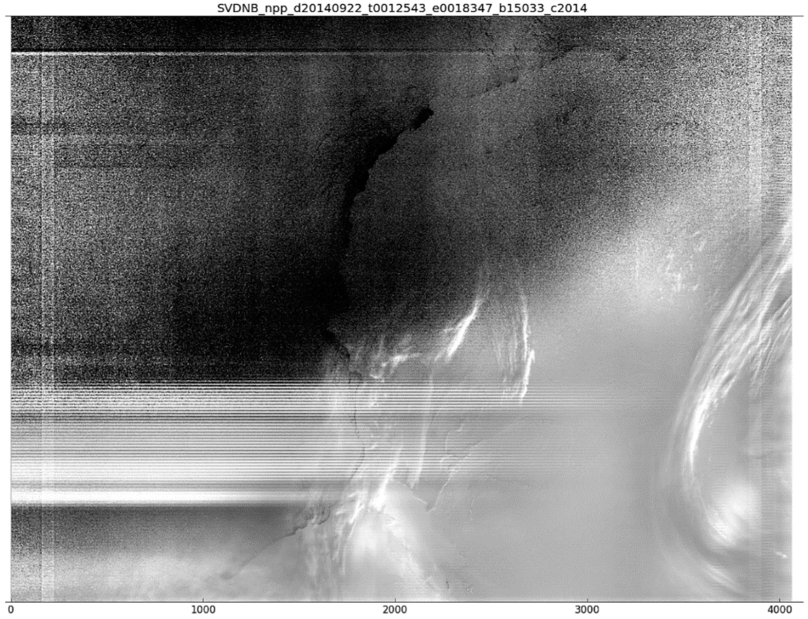
  • In order to observe features in twilight imagery striping we used the Near Constant Contrast algorithm to produce imagery from DNB radiance that minimizes the contrast due to changes in twilight illumination. This algorithm divides the DNB radiance by a factor that is dependent on the computed direct or indirect solar and lunar irradiance. The solar and lunar illumination levels are estimated in the twilight region using a fit to the twilight radiances during new moon [29]. The NCC images here are not from the official version, but use a similar technique to minimize twilight contrast. These NCC images were plotted on a gray scale for evaluation.
  • Along with the radiance plots, we evaluated the associated geolocation to understand the solar or lunar illumination conditions associated with a particular striping artifact. This provides clues as to the root cause of the artifact.
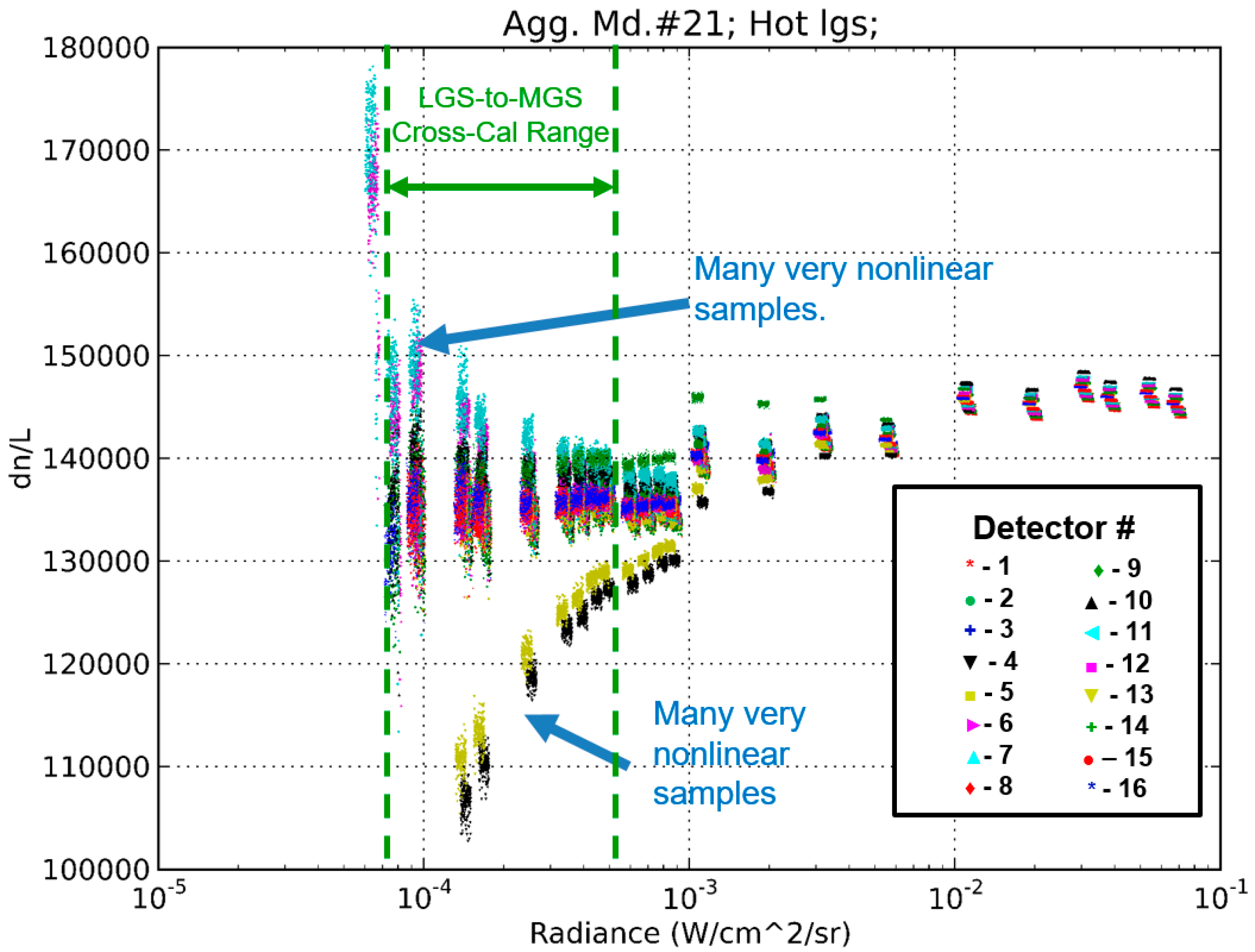
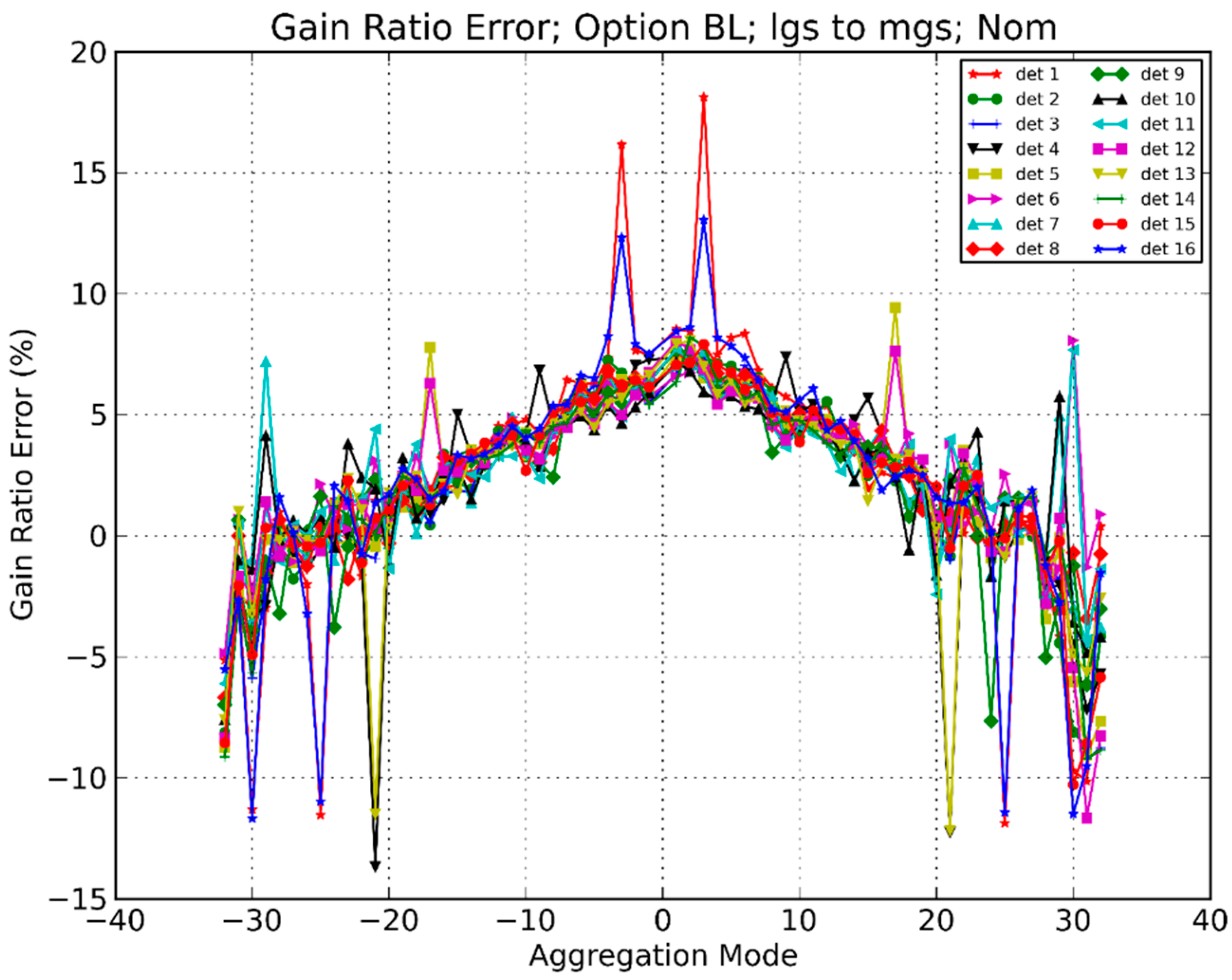
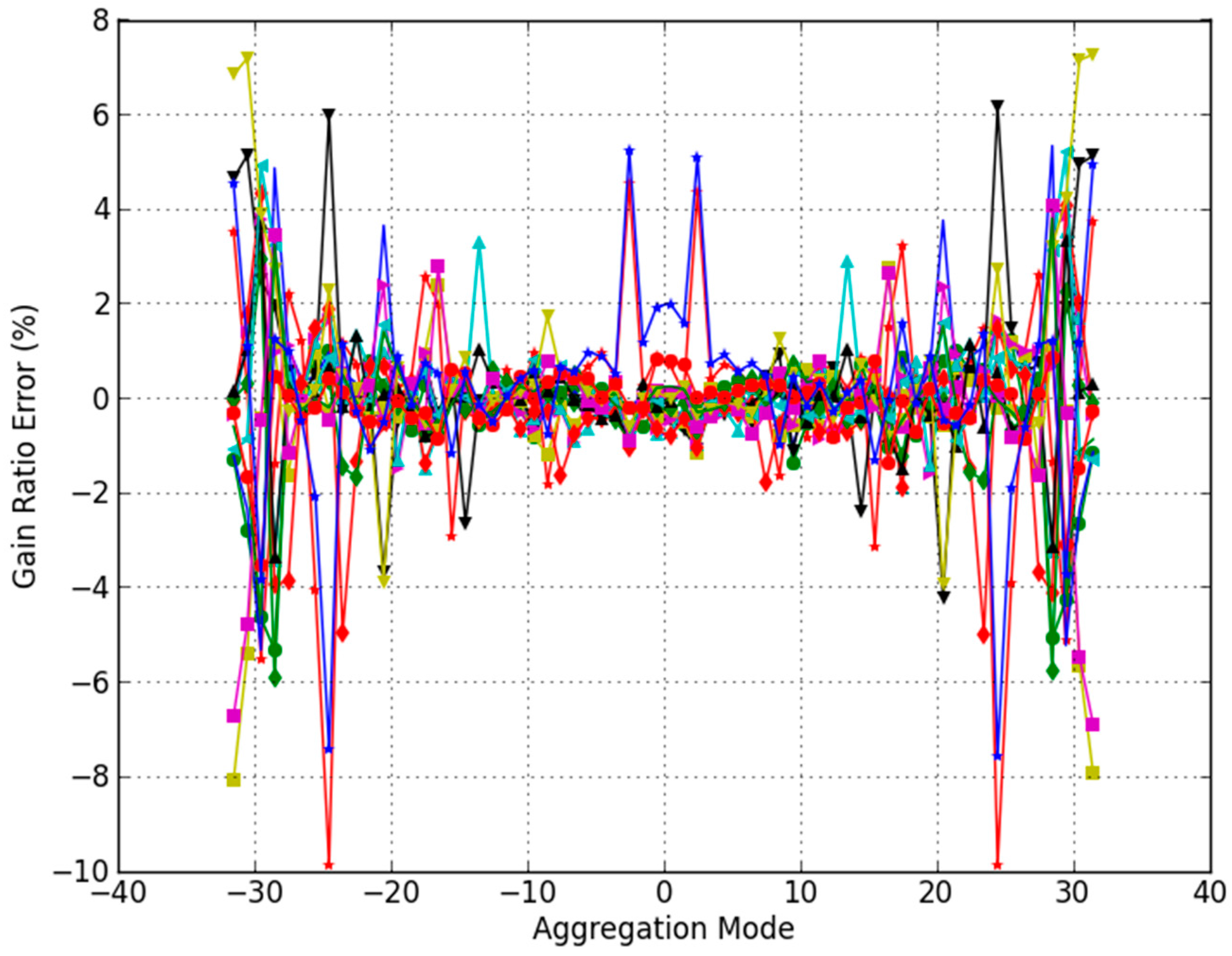
  • We collected and analyzed several days of on-board calibrator data, and in some cases calibrated the counts into radiances using nominal linear calibration coefficients. We produced plots of this cal sector data as a function of time, ASN and/or detector number. In some cases we simulated the calibration process by computing gain ratios and offsets. The on-board calibrator data reveals uncertainties in the calibration process that can lead to striping.
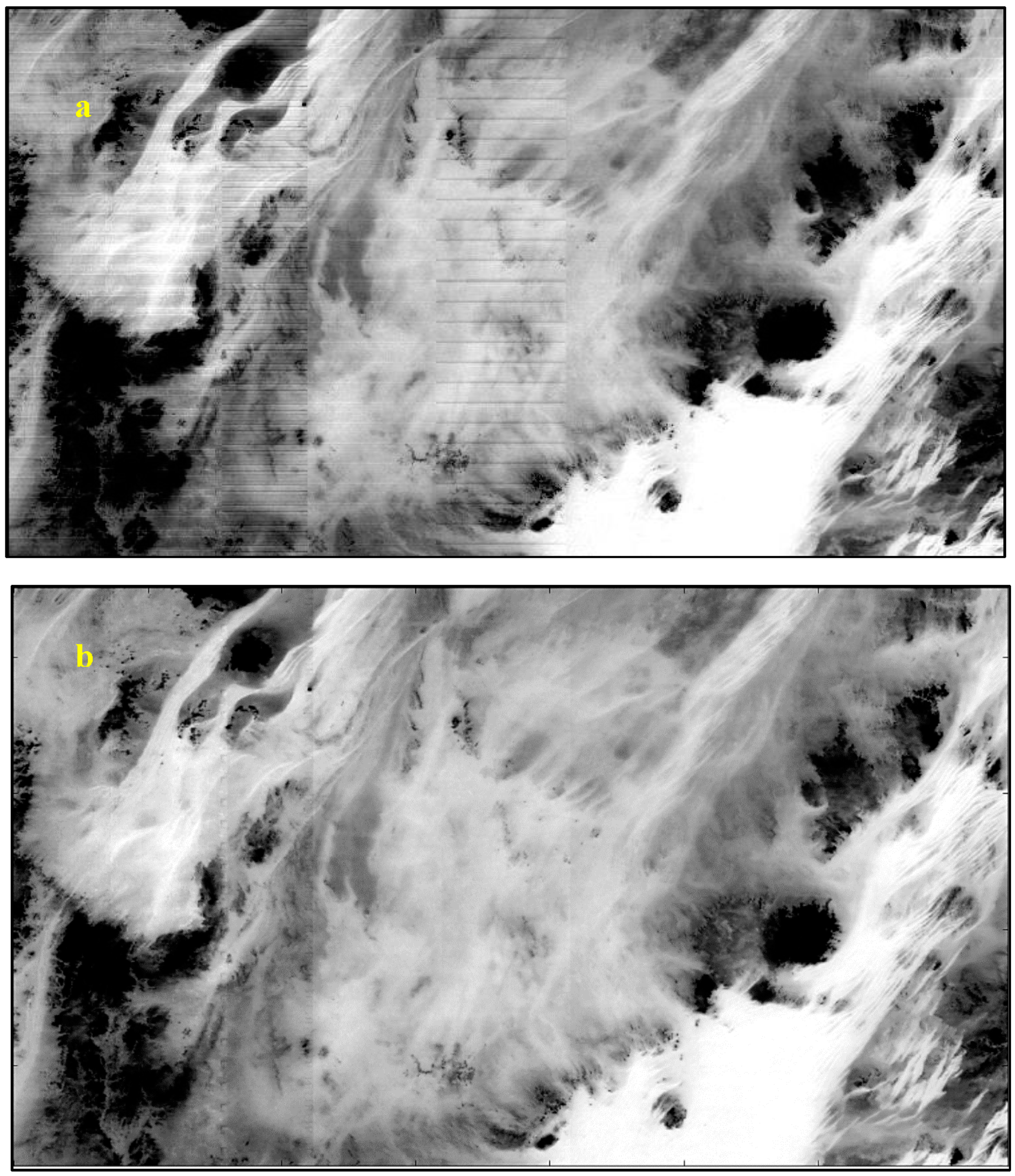
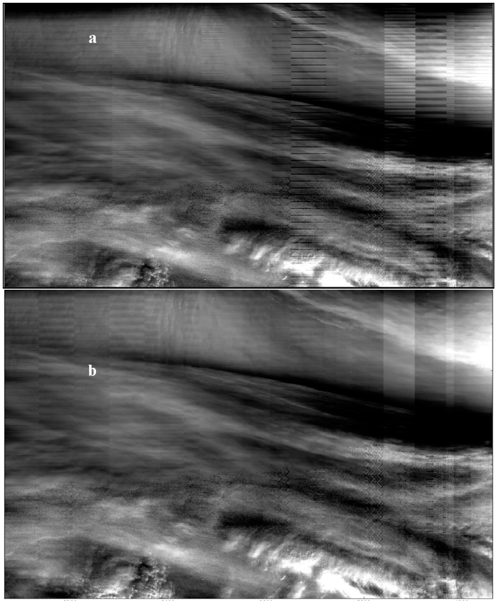
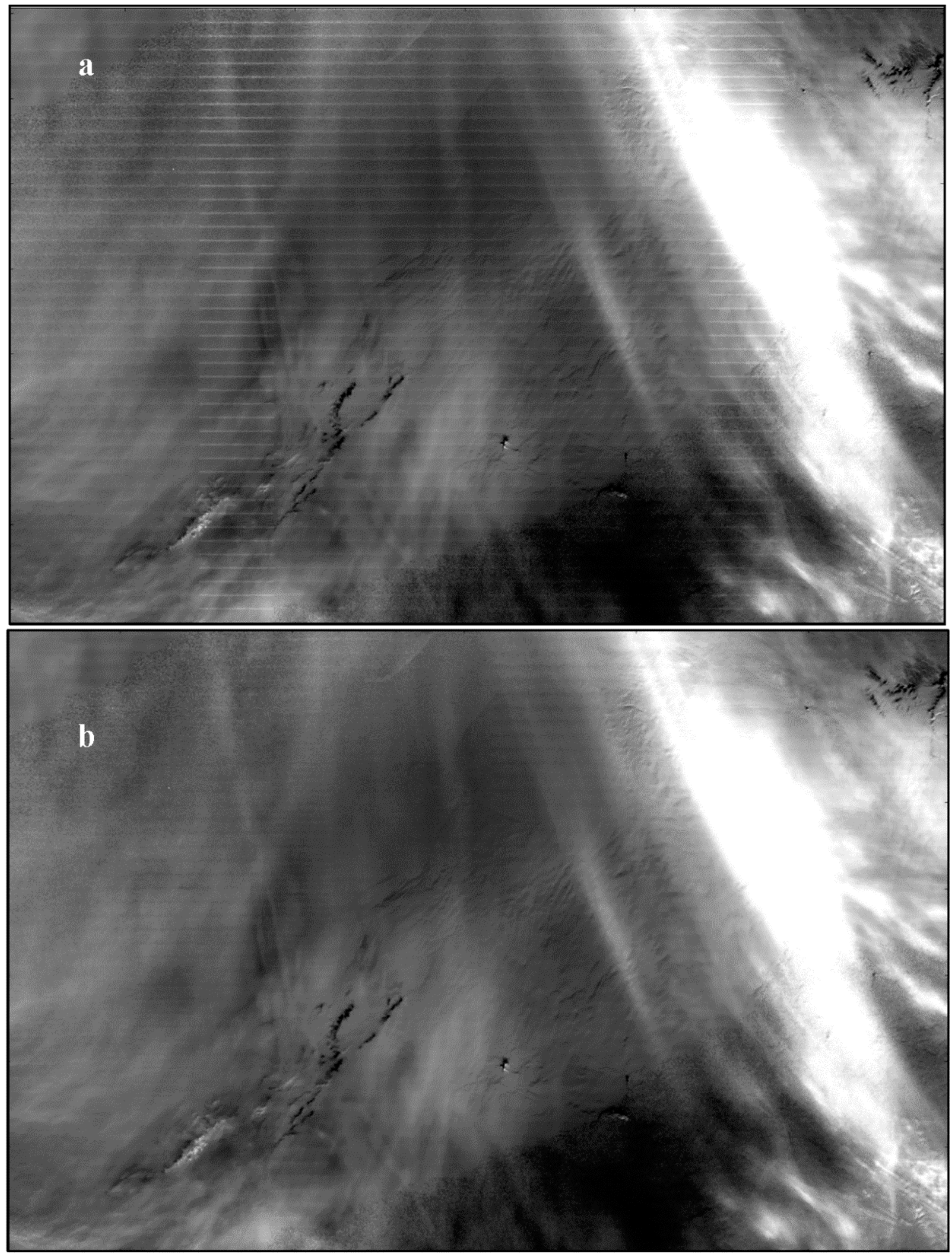
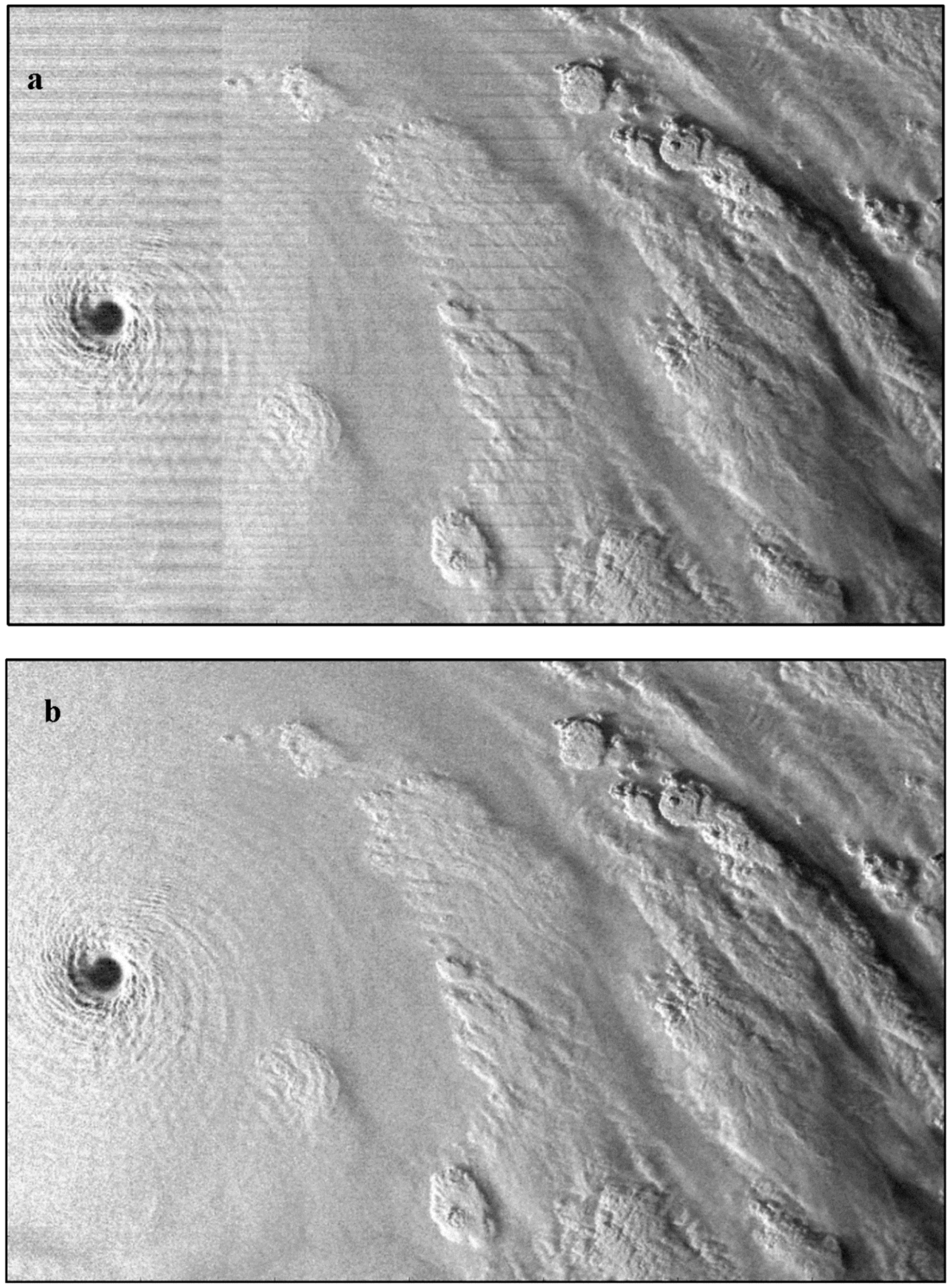
  • We applied the HMM algorithms to SDR data where striping was found and compared the uncorrected images with the corrected images plotted over the same radiance range. We thus evaluated the performance of the destriping algorithm. We also plotted the correction tables used because the detector-to-detector variation seen in the plots are a characterization of the level of striping produced by the DNB.

3. Results

3.1. Survey of DNB Imagery

Nonuniformities, including striping and discontinuities at aggregation zone boundaries have been observed in all DNB SDR calibrated radiances. The effects are generally stronger nearer to the edges of the swath, but can be seen in many cases nearer to the center. Daytime, twilight and nighttime scenes will be considered individually. Desert scenes, and particularly the Sahara Desert, provide relatively uniform targets to evaluate non-uniformities, and some of these scenes are used in the following cases. Polar ice scenes also provide relatively uniform targets to consider. However, even for less uniform scenes, strong non-uniformities are sometimes observed, and these non-uniformities make interpretation of imagery difficult. We include some of these more variant scenes as a way of illustrating the challenges faced by operational users of DNB imagery.
All examples shown here depict radiance values from the DNB SDR, and have not been projected onto a mapping grid. The along-track direction is shown vertically and the in-scan direction is shown horizontally. The reason for this is to preserve the relationship between pixels and detectors in the along-track direction and the aggregation zones in the horizontal direction. Map projections rotate the image and so these relations become less apparent. The radiance range present in the scene is given in the caption.

3.1.1. Observations for Daytime Scenes

Others have observed that daytime VIIRS RSB calibrated radiance scenes exhibit much less striping than MODIS [30,31], and these artifacts generally are not apparent unless extreme contrast stretching is performed. Since the DNB LGS gain calibration uses the same process as the other RSBs, it would be expected to have similar performance in this regard, but we have found that this is not so. The striping pattern we observed repeats every 16 pixels in the vertical direction, indicating that it is caused by variations in calibration over the 16 DNB detectors. Similar striping is seen symmetrically in the corresponding aggregation zones at the other side of nadir in the scan. In all, striping affects 42% of daytime scenes, and is apparent in 18 of the 32 aggregation zones.

3.1.2. Observations for Twilight Scenes

Evaluating nonuniformity for twilight is more difficult for two reasons: the twilight is observed for only a short period in the orbit; in the twilight region there are no radiometrically uniform scenes because of the steep change in radiance as day transitions to night (or vice versa). However, it is an important assessment to make, given that twilight observations dominate the imagery available to Alaska Region operational weather, aviation, and sea ice forecasters (heavy consumers of DNB imagery) during the winter season. In order to observe features in twilight, the Near Constant Contrast algorithm is used to produce imagery from DNB radiance. An NCC image is shown in Figure 2.
The NCC twilight image in Figure 2 contains striping that is strongest on the right side near the end of scan. The transition separating the MGS and the LGS data is shown with a light blue line. The transition occurs where MGS is close to saturation, and this transition is not directly triggered by solar angles.
In the LGS region the image appears grainier because LGS is at low end of its dynamic range and therefore has a lower signal-to-noise ratio (SNR). The striping in the MGS is similar to the striping in the LGS. This is not surprising, because even if the gain ratios were perfect, any gain errors in LGS are transferred to the MGS via the multiplication of the MGS radiance by the gain ratio. There is, however, a vertical zigzag artifact in the LGS that is not seen in the MGS. The likely cause of this artifact will be discussed later in this paper.
Figure 3 shows most of the same DNB scans as Figure 2, but shifted to the left so that the center is near nadir. The ground track location is shifted deeper into the twilight than the end-of-scan. There is striping here across the entire swath. The very bright streak of light on the right side of the image is an example of the Aurora Australis. Other fainter streaks of the aurora appear across the entire image. Surface features of Antarctica include some mountains showing through the ice sheet. The transition separating the MGS and the LGS data is again shown with a light blue line, and the transition separating HGS and MGS is shown as a green line. It is remarkable that all three gain stages appear here in one image and the dynamic range of the radiance shown here is about three orders of magnitude. Twilight images such as this present the biggest challenge for destriping algorithms. Notice that the striping patterns in the LGS, MGS and HGS are similar. Again, this shows that much of this striping is transferred from a lower gain stage to the higher gain stage through the gain ratios.

3.1.3. Observations for Nighttime Scenes

Nighttime DNB scenes are almost entirely relegated to the HGS (with the exception of some very bright gas flares and fires). Generally, nighttime HGS images contain stronger striping than MGS or LGS for two reasons: first, the HGS contains the non-uniformities produced by the LGS calibration as well as the two cross-calibrations; second, the HGS is the only stage where the dynamic range extends into total darkness, so that offset errors appear prominently in the darkest scenes. Figure 4 shows a DNB scene during the new moon over the southeastern Atlantic Ocean. Here, the only source of ambient illumination is nightglow (chemiluminescent airglow) and all other natural illumination from sources other than the sun, the moon or auroras, including, stellar light and zodiacal light. [1,3]. Even by this faint illumination which resides at 10% of the minimum required DNB radiance threshold, cloud features are easily distinguished in the image. However, noise and striping artifacts are prominent throughout the scene.
Figure 5 was collected on 7 October 2014 showing Typhoon Vongfong around the time of its maximum intensity in the Pacific Ocean northeast of the Philippines while illuminated by a nearly full moon. As in Figure 1, gain striping dominates the image and shows that even with the brightest nighttime images, there is significant striping present. This storm had a remarkably concentric structure in ridges in this image—much more so than the daytime VIIRS overpass from 12 h before or after this overpass. Whereas visible imagery of storms reveal structural features that are not seen in the emissive IR imagery, striping makes it more difficult to interpret these fine features, particularly when the striping aligns with naturally occurring banded structures associated with storm dynamics. Furthermore, with striping it is more difficult to design new algorithms that can make use of moonlight reflectance combined with thermal emissive data to better understand such storm systems (e.g., the Dvorak technique [32]).
Figure 6 shows an image of the Ross Sea and Antarctica on 25 June 2015 under quarter moon illumination. In areas where the stray light correction is applied (over approximately the lower two thirds of the image) there are significant residual nonuniformities that were not corrected by the stray light correction. These nonuniformities are likely at least partly due to changes in the stray light between the time that the correction tables were determined and when they were applied [1,10,22]. There is also striping in the upper third of the image similar to what appears in Figure 1.

3.2. Evaluating Causes of Striping and Nonuniformities

It has been noted from several sources that the cause of striping may be that drifts occur over the long monthly cadence of the calibration table update [15,17]. This could explain the striping in the MGS and HGS scenes, but it does not explain striping in the LGS that has a much shorter cadence, the same as the other RSB. In discussing the LGS dark cal sector data, we have noted previously that differences between the SV and SD offsets could not cause significant striping, but there is noticeable striping in LGS scenes, greater than 10% in several places and therefore there must be another cause [5]. We have also noticed by comparing the scenes with a similar ones from 31 days later that the fixed patterns are almost identical for both MGS and LGS. Therefore, there seems to be a systematic error other than drifts that is occurring in both the SD LGS calibration and the LGS-to-MGS cross-calibration. The two dates that were separated by 31 days were at or close to new moon, so lunar stray light was not an issue. However, the DNB cal sectors are sensitive to lunar stray light reflecting off the Earth during a quarter moon or full moon [17].

3.2.1. Stray Light in the Cross-Calibration

The VIIRS SDR Cal/Val Team performed analysis of the DNB gain ratios using the twilight Earth-view data as described above in Original DNB Calibration Process. The gain ratios changed in the first month by as much as 1.7%, with the biggest changes in the aggregation zones near the edges of the swath. The largest changes were in the MGS/LGS gain ratios. For most of the aggregation modes the gain ratios did not change by more than 0.5% over one month [33]. The analysis also revealed that differences in the details of the methodology for calculating the gain ratio look-up tables could change the amount of striping seen in the DNB radiances produced using those tables [34]. There were fluctuations in the gain tables reported during the first year [10] as the calibration methodology was being refined.
We mentioned in the discussion of the RSBAutoCal that during the day there is enough signal in the SD cal sector to produce a gain ratio between the MGS and LGS, and in the SV and BB there is enough signal to determine a gain ratio between the MGS and HGS. Ideally none of these signals should exist if VIIRS were a perfect optical design, so these signals are, strictly speaking, all stray light contamination. After all, the SV should be as dark as space, and the black body should obviously be black for visible and near-infrared wavelengths, and further there is a baffle to prevent solar illumination from striking the BB.
Unfortunately, the SD HGA and HGB signals saturate through most of the daytime, but there are two brief periods per orbit over the twilight region where they do not. However, these are the same periods where direct solar light enters the scan cavity and creates stray light [23]. As can be seen in Figure 7 the resulting HGA/HGB ratios are not consistent for two different day-to-night transitions, a clear sign of stray light issues [19]. These are during the period when the satellite is passing over the terminator from the day to night (the satellite is still in full sunlight). In the first example (a), the ratios at the beginning are around 0.955, which is probably close to the true HGA/HGB gain ratio. However, as the satellite moves deeper into twilight the ratio drops to 0.925. The actual response of the detectors would never change so suddenly, so this drop is apparently due to the difference between the stray light on HGA relative to HGB.
The same is true regarding the difference between stray light on MGS relative to HGA or HGB. In the second day-to-night transition the ratios drop off sooner, possibly because the Earthshine signal is weaker here. For the night-to-day transition, there are only a few unsaturated high gain scans, and many orbits would be required to cover all the ASNs. Therefore, using the SD for determination of gain ratios may be difficult. It may be possible, however, to use the HGA/HGB ratio as a discriminator to detect stray light contaminated data used for HGS/MGS gain ratio computation. Also, by comparing the SV and BB sneak-path stray light signal to the SD signal, a signal-to-stray-light ratio could be computed, and used for filtering. However, neither of these discrimination techniques are used in the current RSBAutoCal algorithm or the Land SIPS automatic calibration. Therefore, not taking stray light contamination into account could lead to striping and bias in the HGS calibration.
Because of these inconsistencies, the authors believe that if BB and SV data were to be used in cross-calibration to determine gain ratios in RSBAutoCal, this would make striping and non-uniformities even worse than they now are, and would also cause more calibration bias. The VIIRS SDR Cal/Val Team has reported problems with this method, and it therefore has not been activated in the RSBAutoCal [20].

3.2.2. Residual Uncorrected Stray Light in the Earth-View

The DNB stray light correction works very well in removing the effects of stray light, but it is not perfect [1,10,22]. There are at least four shortfalls to this method:
  • The correction uses “dark” new moon scenes to characterize the background stray light, but in reality these scenes are not completely dark, since they contain variable amounts of nightglow. The nightglow is estimated from areas where there is no stray light, but since nightglow is not uniform over the scene [31] this variation leads to over/under-correction.
  • The correction look-up tables are constructed as a function of solar zenith angle. In reality, stray light intensity is also a function of solar azimuth angle, and this changes seasonally over the year. This azimuthal dependence is handled empirically; via monthly updates of look-up tables but for times between these synoptic updates the changes in actual stray light cause over/under-correction. This can be somewhat alleviated by taking advantage of the year-to-year 9-days shift in the lunar cycle and using tables created from the previous years. This assumes, however, that the stray light does not change long-term from year to year for other reasons.
  • The stray light cannot be characterized for scenes with twilight illumination, so correction in these areas are estimated either through extrapolation [22] or by setting it to a constant based on the solar zenith angle [10]. Neither of these estimates are perfect, and so this results in residual over/under-correction.
  • Changes in offset between the time the correction tables are made and when they are applied can cause additional striping due to drifts in offset described previously. This is because there is striping in the signal used to estimate airglow, and these offset errors become a part of the correction tables. When the offsets drift, their effect remains in the tables and it creates additional striping in the stray light corrected scene.
The combined effect of all of these factors are seen in Figure 6. Regarding item #3, there is a stray light feature in the twilight region that appears for at least part of the year that is seen only in the southern hemisphere and becomes most prominent in from September through December [35]. It does appear, however, in a weaker form in other months and was first observed in an image from 19 July 2012 [22]. Figure 8 shows an NCC image containing this feature. The artifact affects about 1.2 million km2 per orbit, and appears in every orbit over the same solar zenith angles. Because of the twilight background, it cannot be easily characterized, and thus cannot be easily corrected [35].

3.2.3. Electronic Effects—Hysteresis and Crosstalk

Another problem with the stray light correction is the so-called solar diffuser stray light. This is only seen in the southern hemisphere and begins when direct solar irradiance starts to shine on the SD [10,22]. After studying this effect carefully, however, we now believe that it is probably not, in fact, stray light at all, but is actually an electronic effect. It is indeed related to the strong SD irradiance, but as noted in [22], there is a 72 scan aggregation mode dependent modulation in the SV which shows that this is at least partly an electronic effect. The effect begins abruptly on a single scan, which is not consistent with stray light. If this were, in fact, solar stray light, then the onset should be gradual, extending over about 0.5° (the diameter of the solar disk). Also, we would expect SD stray light to be at least somewhat correlated with the SD signal, but instead it is almost flat, except for the aggregation mode dependent modulation.
Another effect that cannot be easily reconciled with the stray light hypothesis is the fact that the SV signal for this onset is about an order-of-magnitude higher than the EV signal for the same scans. There is no easy way to explain such a large change over the short angular distance between the SV and the start of the Earth-view. For these reasons, we now believe that this is caused by saturation of the high gain SD signal from the previous scan. The onset always appears on the next scan after the SD is saturated in high-gain. This saturation apparently is having some type of hysteresis effect on the detectors, causing a bias during the SV and Earth-view that follows it. The exact mechanism is not known, but it could be that saturation may be leaving excess charge on the DNB CCD, which is then discharged over time during the SV cal sector and the beginning of the Earth-view. This hypothesis is consistent with all of the observed effects and is also borne out by the fact that during the Earth-view the offset gradually decreases to almost nothing by the end of scan. If this hypothesis is correct, then the SD cal signal saturation should be used to determine the onset of what we will now high-gain SD saturation hysteresis. Rather than use solar angle to determine offset, the cal sector aggregation sequence number would be used to determine along-track dependence. Errors in determining the SD onset cause the dark vertical band near the bottom of Figure 6 and the light band near the top of Figure 8.
Other hysteresis effects have been observed as well. A dark band appears in the lower left corner in Figure 4. We have observed in very dark scenes that these dark bands repeat every 72 scans and produce a negative bias with increased offset striping. They are associated the calibration cycle when ASN 1 to 4 are active, and so comprise eight scans. They are apparently associated with a negative hysteresis effect in these particular aggregation modes. The effect dissipates by the end of the scan, and this is also consistent with hysteresis. The negative bias is not large, about 1 × 10⁻¹⁰ W∙cm−2∙str−1, but because of the recent interest in studying scenes illuminated by nightglow, this is significant.
Another artifact that is probably crosstalk is the zigzag (or repeating chevron) pattern noted in the LGS in Figure 2. In prelaunch ground testing these were found to be related to crosstalk from the delay in aggregation mode switching relative to the MGS, HGA and HGB. The delay is because the stages are offset on the array, which requires that they be delayed so that they are collocated spatially. The pattern repeats for every scan, and the “zig” is associated with the first eight detectors and the “zag” is associated with the last eight detectors. This occurs because the detectors are read out one at a time from both sides with a delay of one sample time per detector, and the aggregation mode switching produces crosstalk into the LGS readout electronics. Also, we have observed a streaking effect for very bright point sources at night, especially gas flares and lightning. We believe that this is due to some type of hysteresis effect.
None of these effects should surprise anyone with experience working with CCD arrays. These temporal effects are the price one pays for the extremely high resolution and sensitivity that CCD arrays provide. In particular, the DNB CCD read-out and signal aggregation process is complicated by the many ASNs that it cycles through and by its Time Delayed Integration [36]. Timing becomes critical, and is believed to be the cause of the fixed-pattern offsets in the Earth-view [12,15].

3.2.4. Detector Nonlinearity

Characterization of radiometric response was very limited for the S-NPP DNB, but on JPSS-1 much more extensive characterization was done. Analysis showed that there were large nonlinearities in many of the detectors and that these nonlinearities varied among the detectors and among the aggregation modes [37]. These nonlinearities are significant only in the lowest 1% of the dynamic range for each stage, but unfortunately, this is where the cross-calibration occurs. We see this in Figure 9, showing gain as a function of radiance. Note the logarithmic scale for plotting radiance on the x-axis.
Because the gain in the cross-calibration range is not the same as the gain over the other 99% of the dynamic range, gain ratio error occurs and it varies with detector, causing striping. So even if the MGS and HGS response were perfectly linear for all detectors in aggregation mode 21, this gain ratio error would appear in those stages over their entire dynamic range.
The MGS/LGS gain errors resulting from the nonlinearity in cross-calibration range were computed from the radiometric response test data for JPSS-1, and are shown for all the aggregation modes in Figure 10. The individual detector numbers are shown with different colors and symbols. The spread in the detector errors is a proxy for the striping that would result. There is also an apparent overall bias for all detectors that increases to about 7% at nadir.
Relative gain errors in the S-NPP MGS are shown in Figure 11. These were computed by the destriping algorithm that is described in Histogram Matching Method Destriping Algorithm Description. Comparing Figure 10 and Figure 11, the biggest difference is the bias in Figure 10. However, the destriping algorithm can only determine relative error, not bias, so this is to be expected. Otherwise, they are qualitatively similar. The overall magnitude of the spread in detectors is about the same, and the spread tends to increase in the aggregation modes near the ends of the scan. This is the cause of most of the striping seen in Figure 4. Another similarity is the two out-of-family detectors that form the symmetric “horns” seen on both sides of nadir. These “horns” are in aggregation mode 3 and they cause some of the striping seen in Figure 2 and Figure 5.

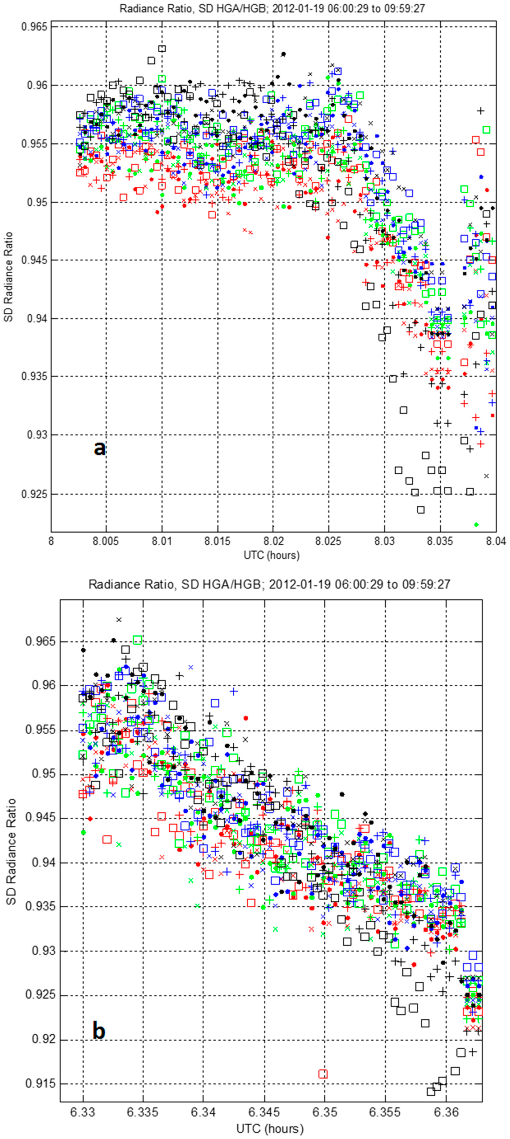
3.2.5. Half-Angle Mirror Side Differences

As described in the Introduction, the HAM rotates, alternating sides for every other scan. The reflectance of both sides of the HAM is measured before launch, and these measurements are used to produce a table used to compensate for the variation in reflectance across the scan and from one mirror side to the other. This correction is called Response Versus Scan (RVS). It is possible, however, for the reflectance of the HAM to change after characterization. This could happen during handling, during launch, or on-orbit. The main cause is expected to be contamination. If one mirror side becomes more contaminated than the other, then there would be a difference between one scan and the next that would appear as an alternating dark/light pattern with a 32 scan-line repetition rate.
Figure 12 shows an image from 28 May 2014 taken by DNB. It is northwest of thunderstorms and depicts gravity waves modulating the intensity of airglow emissions in the upper atmosphere [3,38]. This image has been destriped using the histogram matching method described below. It is obviously extremely noisy relative to any actual variation in the nightglow. However, there does appear to be some gravity waves propagating concentrically from the storms to the southeast. Destriping helps very much here, but on the right there is some modulation that is along-scan (horizontal) and has a 32 scan-line repetition rate that we believe to be due to changes to the RVS. This modulation was not visible before destriping, but is evident here. It could be removed with improvements to the destriping algorithm, and this will be discussed below. Also note the dark horizontal band about 3/4ths of the way down on the image. This is the hysteresis striping that was discussed here previously. This is also not being corrected in the current algorithm but could be with improvements.
It is worth noting here that the effects shown in this image are far below the radiance level for which the DNB was designed to detect. However, with improvements to calibration and to image processing such detection is possible. The gravity waves shown in Figure 12 have a peak-to-valley amplitude of less than 1 × 10⁻¹⁰ W∙cm−2∙str−1, which is also about the magnitude of the RVS error and the hysteresis banding. The SNR here is less than 1, and the only reason that these gravity waves are even faintly visible is because the human mind aggregates the noise. It would be far better to do noise removal through image-processing, but before such noise filtering is done, these other subtle banding and striping errors must be removed.

3.3. Histogram Matching Method Results

We show here a representative example of destriped images from the HMM algorithm. In every case shown, most or all of the striping is removed. The twilight region remains the most challenging. Also, destriping is not shown for scenes where stray light correction has been made. Because the residual striping from the stray light correction varies with region, it is not easily removed using the current HMM technique.
Figure 13 shows the results of this process for the scene shown in Figure 4. This image reveals remarkable detail regarding the cloud formations, given that the only illumination source here is nightglow. The striping has been almost completely eliminated, and this image is truly noise-limited rather than striping limited.
The destriping of some of the nighttime scenes has already been shown in Figure 12. These are both scenes with no lunar illumination, and so the HMM destriping is mostly correcting offset error, except as was noted regarding the 72-scan horizontal dark banding and the mirror side modulations.
Figure 14 shows a scene from 9 September 2014 when the moon is full. It is over the Sahara Desert in southern Egypt. In the uncorrected image striping dominates, but not as much as with new moon scene in Figure 4. This illustrates the magnitude of striping due to gain errors. Figure 15 shows striping in the part of the scan centered on nadir. Gain striping dominates across the entire swath for HGS, but most of it is corrected with HMM destriping.
Figure 16 shows a daytime image, but even with the contrast stretching, there is no visible striping. Some discontinuities can be seen, however, at some of the aggregation zone boundaries.
Figure 17 shows the same twilight scene over the Antarctic as shown in Figure 2 after HMM destriping. Most of the striping has been removed, but some remains. Six orbits of twilight data was used to produce the correction table, but this may not be enough. We are continuing to experiment to determine what ensemble size is sufficient to get optimum twilight striping correction. Also note that the zigzag pattern in the LGS still remain. HMM only deals with striping, not these complex crosstalk artifacts. There are also discontinuities at the boundaries between the aggregation zones. We are working on another algorithm to correct these but it is not yet complete. It has been successful in some cases that will be noted later. Figure 18 shows the twilight scene from Figure 3 after HMM destriping. Most of the striping that appears in Figure 3 has been removed, but there is still some remaining. Note that for there are some aggregation zones that had no striping where there is now some.
We also tested the HMM on scenes with strong lunar illumination. Figure 19 shows the same image of Hurricane Patricia as was shown in Figure 1, but after HMM destriping. In this image the fine ridge structures around the eye of the hurricane can be seen much more clearly.
Figure 20 shows the same image over a wider view so that the dynamic range of the image and of the HMM destriping can be better appreciated. On the right Mexico appears in full darkness with no moonlight. In the middle right, the city lights of the coast city of Acapulco appears, and near the upper right edge Mexico City is seen. There is no visible striping in this image anywhere.
In Figure 4 we noted a light vertical band that appears near the beginning of scan at the left edge. This is aggregation mode 29, which has a strong bias relative to the other adjacent aggregation modes. This light vertical band also appears symmetrically near the end of scan, also in aggregation mode 29. This artifact also appears in Figure 6, Figure 8 and Figure 14. In Figure 17 we noted that by itself HMM destriping was not able to correct this. Notice, however, that this band does not appear in Figure 19 or Figure 20. In this case it has been corrected by a special technique that extends HMM to aggregation mode discontinuities. This technique does not always work, but it did work for this particular scene. We are continuing to test this technique to make it applicable to all scenes and all aggregation mode discontinuities.
Figure 21 shows the same image of Typhoon Vongfong before and after destriping. There is no striping apparent in the corrected image, so the structure of the typhoon can be better analyzed (including the clarity of the transverse banding of the cirrus shield, which is a physical characteristic of the storm [32]). In Figure 19 and Figure 20 the moon is low to the horizon and this creates shadows that highlight Patricia’s structure. However, in the image of Vongfong the moon is nearly full and is almost directly overhead. Therefore, there are fewer dramatic shadows to highlight the structure of Vongfong, and the image is much lower in contrast across the storm top. In such cases of lower contrast, destriping becomes even more important.
Figure 22 shows sea ice illuminated by a full moon off the Antarctic coast on 9 September 2014. In the right half of the images there is a low layer of thin fog over the ice. In many places the fog layer is thin enough to see fractures and leads in the sea ice. The ability to probe through cloud layers that typically are opaque at infrared wavelengths is an important capability of nocturnal DNB imagery at high latitudes [2]. Also, thermal infrared also cannot easily detect ice edges at night. This example highlights the significant benefits of destriping as a prerequisite to automatic image processing to identify quasi-linear features such as ice edges. The amount of blurring in the ice cracks reveals the thickness of the fog as does the shadows at its edges. Detecting these features can be enhanced with advanced image processing techniques, but destriping should be done first for these techniques to work effectively.
The examples of imagery here show the qualitative impact of striping, but it is also important to understand the impact quantitatively, especially when considering the impact to processes that require radiometric accuracy. Figure 23 shows the gain corrections used to correct striping Figure 22 as a percentage of the radiance signal. This shows the quantitative impact of striping as well as the quantitative benefits of correction. Note the similarity with Figure 11 that shows the gain correction for the MGS. From this we conclude that most of the striping in bright nighttime DNB images are caused by gain ratio errors that are transferred from LGS to MGS to HGS. Typically striping over 2% is visible in uniform scenes. Many of the detectors in many of the aggregation modes, especially near the edge of the swath, do not meet these criteria. The striping increases toward the edge of scan as would be expected from the imagery.

4. Discussion

The examples of destriping shown here were produced using our off-line post processing software where a DNB SDR dataset is input, and a corrected SDR is output. Ideally, though, this process would be incorporated into the operational calibration process. In order to do this, it is important that destriping be integrated into the entire calibration process. In this way, the process is done in the proper order. For example, the NCC is produced from the DNB SDR, but once this is done, the NCC imagery cannot be destriped as a post-process because it is projected into the Ground-Track Mercator Projection (this is why the NCC examples shown here must use a simplified off-line version of the NCC algorithm).
Another problem with removing striping as a post-process is that striping from other causes, especially nonlinearity, become mixed with the stray light correction and this striping becomes impressed into the stray light correction tables.
Therefore, we recommend that the HMM destriping algorithm described here be incorporated into the operational software. In the discussion that follows, we consider what would be required to do this.

4.1. Changing the DNB Calibration Process to Reduce Striping

By taking statistics for dark scenes over many orbits of data, a mean nightglow profile could be estimated from the dark noise via the Photon Transfer Curve (PTC) method and this could then be subtracted off [1]. In this way dark DNB imagery for scenes with no lunar illumination could be produced automatically by the calibration process that is both uniform and radiometrically accurate. This could also be done as an offline process for users who work with very dark scenes.
The NASA VCST has reported a 6% to 7% bias when comparing HGS gain computed using the cal sector with the HGS gain determined from the monthly Earth-view cross-calibration [17]. They attribute this to the stray light in the Earth-view cross-calibration [10]. We have shown that there is actually stray light in both the cal sector data and in the Earth-view data, either can cause bias in the cross-calibration, and these levels should be compared to determine which is worse. The Earth-view stray light has been well characterized and an estimate is used in the twilight where cross-calibration occurs [22]. The stray light in the cal sectors have also been extensively characterized. Evaluating these data we have found that in general, the Earth-view data used by the original cross-calibration process has a better signal-to-stray-light ratio than does the SD illuminated by Earthshine. This is not because the stray light is stronger in the SD cal sector, but rather because the Earthshine signal is weaker compared with the Earth-view signal for the same solar angles. Nevertheless, if the stray light discrimination techniques described above were implemented, the SD signal could potentially yield better gain ratios and cause less striping. Also, an improvement to the Earth-view method would to be to perform the HGS/MGS cross-calibration using only the aggregation zones on the left half before nadir (beginning of scan). This would reduce stray light in the gain ratio computation because the calibration modes are reflected on each side of the scan, and because of the angle that the satellite path makes with the terminator, the left side transitions from MGS to HGS sooner, when the stray light is much less [12,13].
The RSBAutoCal was designed to use only cal sector data, because it was presumed that automating the Earth-view cross calibration would be too complicated or would require putting the DNB in a non-operational mode [15,21]. Actually the LGS and MGS data could be enabled to transmit at the same time that the instrument is switched to night mode for every orbit without any special operational procedure. There is a misconception that this requires putting the instrument into a non-operational mode, or that there must be a loss of operational data while doing this. The loss of daytime RSB does occur if in fact the day-to-night mode transition is enabled earlier to allow for LGS-to-MGS cross-calibration [12]. However, if the SD cal sector is used instead only for this MGS/LGS gain ratios, then the night mode can be enabled at the normal time, along with the MGS and LGS data transmission, as long as this transmission is automatically turned off before the SD is illuminated (otherwise the M4 and M5 bands cal sector data would not be transmitted). Allowing MGS and LGS to transmit for the first 35 min of the night mode for every orbit would provide more than enough data for per-orbit MGS to HGS gain ratio updates. Such a change, of course would require that flight operations change the per-orbit command sequence. This data could also be used for MGS offsets for any pixels where there is no electric lights, stray light, solar illumination or lunar illumination and for any LGS pixels at night. However, regardless of whether the cal sector data or the earth view data is used, no MGS to HGS cross calibration should be performed in the southern hemisphere because of the electronic hysteresis discussed in Section 3.2.3 and stray light contamination from the solar diffuser discussed in Section 3.2.2.

4.2. Histogram Matching Method Computational Considerations

The DNB produces about three tera-pixels of imagery per day, presenting an onerous computational task if implemented operationally. There are two parts of destriping:
  • Collecting the ensemble of pixel radiances, filtering the ensemble, producing histograms, and computing correction tables from the histograms.
  • Applying the correction tables to the DNB radiances.
In considering computational costs, one fact to note is that the ensemble of radiances used to compute the correction does not need to come from the set of radiances that are being corrected. There are advantages in using current data, however, because the statistics in the ensemble closely match the statistics of the radiances being corrected. The problem with doing so is that if the ensemble is too small, then it may not have enough data to be statistically robust. We have found that one 5 min granule is large enough to provide a statistically robust ensemble.
There are, however, many cases where one granule is not enough and we must combine several granules together to produce a valid ensemble. This is especially true for the twilight because we separate the twilight into four ensembles equally spaced by solar zenith angle from 85° to 105°. These ensemble must be combined with the corresponding ensembles from other orbit’s twilight crossing.
Because the creation of histograms requires a sorting of the radiances, the computational time to process an ensemble is proportional to the square of the number of elements in it. As such, ensembles must be limited to only a few granules. Processing the twilight corrections require the largest ensembles, and producing the correction tables can take several hours.
The process of applying the corrections is not as computationally intensive as construction of the correction tables, and the computation time is only linearly proportional to the number of pixels being corrected. Therefore there is an advantage to computing the correction tables from a limited sample (e.g., one orbit of nighttime data) and then applying that correction to many other granules (e.g., all the nighttime granules for that date). What we were uncertain of is how stable these corrections are. Are they valid for 6 h, 24 h or 48 h? Surprisingly, we found that they are valid for at least a month, implying that the response drift discussed in Section 3.2.1 and Section 3.2.2 are not as significant as has been previously thought.
We used tables created from the night of 7 October 2014 and applied them to 9 September 2014, and the tables corrected as well as tables produced from the same day. It is important to note here that for both dates the moon was full, and we believe that it is necessary to use tables from dates with similar illumination. However, for the day and the twilight this should not be as important, since the illumination changes slowly with season.
We continue to experiment with the best techniques to use to optimize the HMM destriping. Ideally, these techniques would be incorporated into the operational process directly so that all end-users would have access to the highest quality imagery. If that were to happen, then the computational considerations discussed here would be vitally important to streamlining this process.
HMM in its current instantiation cannot fix all of the nonuniformities in the DNB imagery. For example the zigzag patterns in Figure 17 are not removed by HMM. The 72-scan banding artifact shown in Figure 4 may be correctable with HMM if it were to be treated as a separate ensemble. This hypothesis is currently being investigated. The mirror side modulation shown in Figure 12 could be fixed by treating the detectors on each side as independent, effectively treating the DNB as if it were a 32 detector sensor.
Striping caused by stray light correction residuals can only be removed through improvements to the stray light correction algorithm itself, and some of those proposed changes have been discussed herein.

5. Conclusions

We have considered the design of VIIRS and the DNB with respect to the original DNB calibration algorithm and the new RSBAutoCal algorithm. A review of DNB scenes shows that visible striping exists in the DNB SDR radiances over large parts of the swath for all gain stages from full day through moonless nights, though striping is the worst in the HGS at night. Since striping in DNB daylight scenes (LGS) is much stronger than is seen in other RSB, there is a root cause specific to the DNB. There is strong striping in twilight and night scenes, but with twilight it is only evident when scenes are viewed using NCC.
A study of the three cal sectors (SD, SV, and BB) shows that under dark conditions there are differences of up to 3.5 counts in the daily means of dark offsets. These differences are systematic and remain almost constant for a period of at least one month, and probably much longer. These may represent a proxy for the stability of the differences between the cal sector and the Earth-view, and so is significant in using the cal sector for Earth-view offset correction. Offset correction is key to reducing striping in the darkest scenes, and cal sector data, and because of nightglow, the offset is very difficult to determine using earth view data alone.
The gain ratios between all four of the DNB stages, LGS, MGS, HGA, and HGB were considered for all three of the aforementioned cal sectors. The SD LGS-to-MGS gain ratios for the period when indirect Earthshine light leaks through the attenuation screen and illuminates the SD appear to be stable enough to be useful as an alternative source of cross-calibration data, but by itself, this would not reduce striping because of detector nonlinearity. The HGA and HGB signals are typically saturated except for a brief period which corresponds to strong sneak-path stray light. We believe that sneak-path stray light is responsible for most of the signal seen during the day in the BB and SV cal sectors. Therefore, this stray light does not illuminate the gain stages or the detectors evenly and is not useful for cross-calibration. If the RSBAutoCal algorithm uses these data for cross-calibration, it will likely introduce more striping. The authors therefore do not recommend implementing this part of the RSBAutoCal algorithm. Instead we recommend transmitting MGS and LGS data as a normal part of nighttime operations and using the MGS data for MGS-to-HGS cross-calibration.
The root causes of striping in the DNB imagery were enumerated. These are: offset instability, stray light in the cross-calibration, detector nonlinearity, electronic transients and hysteresis, electronic crosstalk, residual uncorrected stray light in the Earth-view, and uncorrected HAM mirror side modulation. We have shown that stray light correction and destriping are related and should be addressed together. With 3 years of new moon data now available, stray light correction tables that are dependent on solar azimuth angle in addition to solar zenith angle could now be produced, and this would improve the continuity of the correction. Also, based on this study, the signal seen in the southern hemisphere that is associated with the illumination of the solar diffuser is electronic hysteresis. This has been previously treated as stray light, but if the calibration algorithm were to treat it instead as electronic hysteresis, nonuniformity would be reduced.
We tested the effectiveness of various destriping techniques including moment matching and HMM. HMM was found to be the most effective, and the only technique that can cover the huge dynamic range of the DNB. HMM works well in removing most striping, although some striping artifacts remain. Therefore, we continue our investigation of enhanced destriping techniques for producing high-quality DNB imagery. Further, HMM can be used as an effective tool to characterize relative radiometric error as shown in Figure 23. This is a necessary part of an overall strategy to improve the long-term calibration of the instrument and should be a component of any reprocessing of the data record.

Acknowledgments

The work presented in this paper was funded by Renaissance Man Engineering. The authors would like to thank Steve Finley for his work testing the software using the hardware at Colorado State University, Fort Collins, Cooperative Institute for Research in the Atmosphere.

Author Contributions

Stephen Mills performed all sensor analysis and developed and tested the HMM destriping algorithm. Steven Miller evaluated imagery before and after destriping and specified the type of scenes to be tested by this process. Steven Miller then evaluated the quality of the corrected imagery in relation to scientific requirements.

Conflicts of Interest

The authors declare no conflict of interest.

Abbreviations

The following abbreviations are used in this manuscript:
ASN
Aggregation Sequence Number
BB
Black Body
CLASS
Comprehensive Large Array-data Stewardship System
DNB
Day/Night Band
HAM
Half-Angle Mirror
HGA
High-Gain A
HGB
High-Gain B
HGS
High-Gain Stage
HMM
Histogram Matching Method
IDPS
Interface Data Processing Segment
LGS
Low-Gain Stage
MGS
Mid-Gain Stage
MM
Moment Matching
MODIS
Moderate-Resolution Imaging Spectroradiometer
NCC
Near-Constant Contrast
RVS
Response Versus Scan
RSB
Reflective Solar Band
SD
Solar Diffuser
SDR
Senor Data Record
SIPS
Science Investigator-led Processing System
S-NPP
Suomi National Polar-orbiting Partnership
SV
Space View
VCST
VIIRS Science Support Team
VIIRS
Visible Infrared Imaging Radiometer Suite

References

  1. Liao, L.B.; Weiss, S.; Mills, S.; Hauss, B. Suomi NPP VIIRS day and night band on-orbit performance. J. Geophys. Res. Atmos. 2013, 118, 12705–12718. [Google Scholar] [CrossRef]
  2. Miller, S.D.; Straka, W., III; Mills, S.P.; Elvidge, C.D.; Lee, T.F.; Solbrig, J.; Walther, A.; Heidinger, A.K.; Weiss, S.C. Illuminating the capabilities of the Suomi NPP VIIRS Day/Night Band. Remote Sens. 2013, 5, 6717–6766. [Google Scholar] [CrossRef]
  3. Miller, S.D.; Mills, S.P.; Elvidge, C.D.; Lindsey, D.T.; Lee, T.F.; Hawkins, J.D. Suomi satellite brings to light a unique frontier of nighttime environmental sensing capabilities. Proc. Natl. Acad. Sci. USA 2012, 109, 15706–15711. [Google Scholar] [CrossRef] [PubMed]
  4. Baugh, K.; Hsu, F.C.; Elvidge, C.; Zhizhin, M. Nighttime Lights Compositing Using the VIIRS Day-Night Band: Preliminary Results. Proc. Asia Pac. Adv. Netw. 2013, 35, 70–86. [Google Scholar] [CrossRef]
  5. Mills, S.; Miller, S. VIIRS Day-Night Band (DNB) calibration methods for improved uniformity. Proc. SPIE 2014, 9218. [Google Scholar] [CrossRef]
  6. Miller, S.D.; Turk, F.J.; Lee, T.F.; Hawkins, J.D.; Velden, C.S.; Schmidt, C.C.; Prins, E.M.; Haddock, S.H. The origin of sensors: Evolutionary considerations for next-generation satellite programs. American meteorological society. In Proceedings of the 14th Conference on Satellite Meteorology and Oceanography, Atlanta, GA, USA, 28–30 January 2006.
  7. Baker, N. Instrument overview. In Joint Polar Satellite System (JPSS) VIIRS Radiometric Calibration Algorithm Theoretical Basis Document ATBD, rev. C; Goddard Space Flight Center: Greenbelt, MD, USA, 2013; pp. 12–24. [Google Scholar]
  8. Baker, N. Day-night band FPA and Interface Electronics. In Joint Polar Satellite System (JPSS) VIIRS Radiometric Calibration Algorithm Theoretical Basis Document ATBD, rev. C; Goddard Space Flight Center: Greenbelt, MD, USA, 2013; pp. 25–29. [Google Scholar]
  9. Miller, S.W.; Jamilkowski, M.; Grant, K. Joint Polar Satellite System (JPSS) Common Ground System (CGS) Architectural Overview and Tenets. Available online: http://www.jpss.noaa.gov/AMS_2014/Presentations/31_JPSS_CGS_Overview_and_Architectural_Tenets.pdf (accessed 1 Dec 2015).
  10. Lee, S.; Chiang, K.F.; Xiong, X.; Sun, C.; Samuel, A. The S-S-NPP VIIRS Day-Night Band On-Orbit Calibration/Characterization and Current State of SDR Products. Remote Sens. 2014, 6, 12427–12446. [Google Scholar] [CrossRef]
  11. Baker, N. Day-night band calibration. In Joint Polar Satellite System (JPSS) VIIRS Radiometric Calibration Algorithm Theoretical Basis Document ATBD, rev. C; Goddard Space Flight Center: Greenbelt, MD, USA, 2013; pp. 102–109. [Google Scholar]
  12. Mills, S.; Jacobson, E.; Jaron, J.; McCarthy, J.; Ohnuki, T.; Plonski, M.; Searcy, D.; Weiss, S. Calibration of the VIIRS Day/Night Band (DNB). In Proceedings of the 6th Annual Symposium on Future National Operational Environmental Satellite Systems-NPOESS and GOES-R, Atlanta, GA, USA, 17–21 January 2010.
  13. Geis, J.; Florio, C.; Moyer, D.; Rausch, K.; de Luccia, F. VIIRS day-night band gain and offset determination and performance. Proc. SPIE 2012, 8510, 8510–8512. [Google Scholar]
  14. Baker, N. Solar Diffuser Calibration Multi-Orbit Aggregation. Joint Polar Satellite System (JPSS) VIIRS Radiometric Calibration Algorithm Theoretical Basis Document ATBD, rev. C; Goddard Space Flight Center: Greenbelt, MD, USA, 2013; p. 145. [Google Scholar]
  15. Rausch, K.; Houchin, S.; Cardema, J.; Moy, G.; Haas, E.; de Luccia, F.J. Automated calibration of the Suomi National Polar-Orbiting Partnership (S-NPP) Visible Infrared Imaging Radiometer Suite (VIIRS) reflective solar bands. J. Geophys. Res. Atmos. 2013, 118, 13434–13442. [Google Scholar] [CrossRef]
  16. Mills, S. VIIRS DNB Stray Light Anomaly Analysis (DR4623); NOAA internal document # ND3475506; NOAA: Silver Spring, MD, USA, 2012.
  17. Lee, S.; McIntire, J.; Oudrari, H.; Schwarting, T.; Xiong, X. A New Method for Suomi-NPP VIIRS Day–Night Band On-Orbit Radiometric Calibration. IEEE Trans. Geosci. Remote Sens. 2014. [Google Scholar] [CrossRef]
  18. Lee, S. VIIRS F1 Day Night Band Offset Determination: VROP702 vs. Pitch Maneuver; NOAA Internal document, NICST_REPORT_POST_12_011; NOAA: Silver Spring, MD, USA, 2012.
  19. Mills, S. VIIRS DNB Cross-Stage Gain Calibration Using Earthshine on Solar Diffuser; NOAA internal document # ND3475507; NOAA: Silver Spring, MD, USA, 2012.
  20. Haas, E. RSBAutoCal Status and Path Forward, STAR JPSS Annual Science Team Meeting, 26 August 2015. Available online: http://www.star.nesdis.noaa.gov/star/documents/meetings/2015JPSSAnnual/ (accessed on 23 November 2015).
  21. Baker, N. Description of theoretical basis for Reflective Solar Band (RSB) Automatic calibration (RSBAutocal) algorithm. In Joint Polar Satellite System (JPSS) VIIRS Radiometric Calibration Algorithm Theoretical Basis Document ATBD, rev. C; Goddard Space Flight Center: Greenbelt, MD, USA, 2013; pp. 154–161. [Google Scholar]
  22. Mills, S.; Weiss, S.; Liang, C. VIIRS day/night band (DNB) stray light characterization and correction. Proc. SPIE 2013, 8866. [Google Scholar] [CrossRef]
  23. NOAA Comprehensive Large Array-Data Stewardship System. Available online: www.class.ngdc.noaa.gov/saa/products/welcome (accessed on 1 December 2015).
  24. Community Satellite Processing Package. Available online: http://cimss.ssec.wisc.edu/cspp/ (accessed on 1 December 2015).
  25. Gumley, L. CSPP polar-orbiting satellite software and products. In Proceedings of the 2015 CSPP/IMAPP Users’ Group Meeting, Darmstadt, Germany, 14–16 April 2015.
  26. Bouali, M.; Ladjal, S. Toward Optimal Destriping of MODIS Data Using a Unidirectional Variational Model. IEEE Trans. Geosci. Remote Sens. 2011, 49, 2924–2935. [Google Scholar] [CrossRef]
  27. Mills, S. VIIRS Day-Night Band destriping methods for improved uniformity. GSICS Q. 2015, 9. [Google Scholar] [CrossRef]
  28. Horn, B.K.P.; Woodham, R.J. Destriping Landsat MSS images by histogram modification. Comput. Gr. Image Process. 1979, 10, 69–83. [Google Scholar] [CrossRef]
  29. Liang, C.K.; Mills, S.; Hauss, B.I.; Miller, S.D. Improved VIIRS Day/Night Band Imagery with Near-Constant Contrast. IEEE Trans. Geosci. Remote Sens. 2014, 52, 6964–6971. [Google Scholar] [CrossRef]
  30. Bhatt, R.; Doelling, D.R.; Wu, A.; Xiong, X.; Scarino, B.R.; O’Haney, C.; Gopalan, A. Initial Stability Assessment of S-NPP VIIRS Reflective Solar Band Calibration Using Invariant Desert and Deep Convective Cloud Targets. Remote Sens. 2014, 6, 2809–2826. [Google Scholar] [CrossRef]
  31. Cao, C.; de Luccia, F.J.; Xiong, X.; Wolfe, R.; Weng, F. Early on-orbit performance of the visible infrared imaging radiometer suite onboard the Suomi national polar-orbiting Partnership (S-NPP) satellite. IEEE Trans. Geosci. Remote Sens. 2014, 52, 1142–1156. [Google Scholar] [CrossRef]
  32. Velden, C.; Harper, B.; Wells, F.; Beven, J.L., II; Zehr, R.; Olander, T.; Mayfield, M.; Guard, C.; Lander, M.; Edson, R.; et al. The Dvorak Tropical Cyclone Intensity Estimation Technique, A Satellite-Based Method that Has Endured for over 30 Years. BAMS 2006. [Google Scholar] [CrossRef]
  33. Mills, S.; Liang, C. VIIRS DNB Cross-Stage Calibration Coefficient Ratio Change in 1 Month; NOAA internal document # ND3475514; NOAA: Silver Spring, MD, USA, 2012.
  34. Mills, S.; Liang, C. Comparison of DNB Inter-Stage Gain Ratios; NOAA internal document # ND3475668; NOAA: Silver Spring, MD, USA, 2012.
  35. Liao, L.; Weiss, S.; Liang, C. DNB performance. In Proceedings of 2013 Suomi NPP SDR Science and Products Review, College Park, MD, USA, 18–20 December 2013.
  36. McCarthy, J.K.; Jacobson, E.J.; Kilduff, T.M.; Estes, R.W.; Levine, P.A.; Mills, S.; Elvidge, C.; Miller, S.D. On the potential to enhance the spatial resolution of the day-night band (DNB) channel of the visible and infrared imaging radiometer suite (VIIRS) for the second joint polar satellite system (JPSS-2) and beyond. Proc. SPIE 2013, 8866. [Google Scholar] [CrossRef]
  37. Mills, S. JPSS-1 VIIRS DNB, prelaunch tests & performance. In Proceedings of 2015 STAR JPSS Annual Science Team Meeting, College Park, MD, USA, 24–28 August 2015.
  38. Miller, S.D.; Straka, W.C., 3rd; Yue, J.; Smith, S.M.; Alexander, M.J.; Hoffmann, L.; Setvák, M.; Partain, P.T. Upper atmospheric gravity wave details revealed in nightglow satellite imagery. Proc. Nat. Acad. Sci. USA 2015, 112. [Google Scholar] [CrossRef] [PubMed]
Figure 1. Nighttime scene of Hurricane Patricia with striping from 23 October 2015 at 07:45 UTC over the Pacific Ocean west of Mexico during a waxing gibbous moon. The radiances are plotted on a linear scale over the range of 0 to 6 × 10⁻⁹ W∙cm−2∙sr−1 from black to white. The 500 by 700 pixels image is at left edge start of scan.
Jimaging 02 00009 g001
Figure 2. Near Constant Contrast (NCC) twilight scene with striping from 22 September 2014 at 00:19 UTC in a region of Antarctica. The image is 650 by 1000 pixels and the right edge is the end of scan. The blue line shows the transition between the Mid-Gain Stage (MGS) above the line and the Low-Gain Stage (LGS) below it. The median radiance in this image is about 5 × 10⁻⁴ W∙cm−2∙sr−1.
Jimaging 02 00009 g002
Figure 3. NCC twilight scene over Antarctica with striping from 22 September 2014 at 00:19 UTC. The image is 700 by 1100 pixels and is centered near nadir. The median radiance in this image is about 1 × 10⁻⁵ W∙cm−2∙sr−1.
Jimaging 02 00009 g003
Figure 4. Image collected under new moon (i.e., nightglow illumination) conditions on from 28 May 2014 at 01:38 UTC in a region of the southeastern Atlantic. Radiances are plotted on a linear scale over the range of −1.0 × 10⁻¹⁰ to 3.3 × 10⁻¹⁰ W∙cm−2∙sr−1 black to white. The 1000 by 1900 pixel image is at start of scan.
Jimaging 02 00009 g004
Figure 5. Nighttime scene of Typhoon Vongfong with striping from 7 October 2014 at 17:03 UTC from black to white. The image is 656 by 940 pixels and is located near center of swath. Gray scale is linear from 2 × 10⁻⁹ to 3.6 × 10⁻⁸ W∙cm−2∙str−1.
Jimaging 02 00009 g005
Figure 6. Nighttime scene with striping from 25 June 2015 at 15:32 UTC, showing cloud cover over the Ross Sea and Antarctica. . This images uses NCC and shows1275 by 1900 pixels.
Jimaging 02 00009 g006
Figure 7. HGA/HGB ratio for two day-to-night transitions. Each of the 16 detectors has a different color/symbol combination, and this plot illustrates the spread (or striping) by detector.
Jimaging 02 00009 g007
Figure 8. NCC image of stray light artifact on 22 September 2014 00:17 UTC over Antarctica.
Jimaging 02 00009 g008
Figure 9. LGS nonlinearity for JPSS-1 in aggregation mode 21 showing gain as a function of radiance.
Jimaging 02 00009 g009
Figure 10. JPSS-1 Day-Night Band (DNB) MGS/LGS gain ratio error, computed from radiometric response tests.
Jimaging 02 00009 g010
Figure 11. S-NPP MGS gain ratio errors computed by on-orbit destriping algorithm.
Jimaging 02 00009 g011
Figure 12. Gravity waves seen in nightglow nighttime scene over Africa, 28 May 2014 at 01:23 UTC. Image has been destriped but there appears to be residual mirror-side dependent banding.
Jimaging 02 00009 g012
Figure 13. Nighttime scene (a) with striping and (b) with HMM destriping correction from 28 May 2014 at 01:38 UTC.
Jimaging 02 00009 g013
Figure 14. Nighttime scene (a) with striping and (b) with Histogram Matching Method (HMM) destriping, from 17 June 2014 at 23:46 UTC in a region of the Sahara Desert in southern Egypt.
Jimaging 02 00009 g014
Figure 15. (a) Nighttime scene before destriping and (b) after destriping, from 9 September 2014 at 00:32 UTC in the Sahara Desert in Libya. The radiances are plotted on a linear scale over the range of 0 to 4.1 × 10⁻⁸ W∙cm−2∙sr−1 from black to white. The image is 500 by 750 pixels and is centered at nadir.
Jimaging 02 00009 g015
Figure 16. Daytime scene (a) with striping and (b) with HMM destriping, from 28 May 2014 at 12:32 UTC in a region of the Sahara Desert in southeastern Libya. The radiances are plotted on a linear scale over the range 3.6 to 5.8 × 10⁻³ W∙cm−2∙sr−1 from black to white. The image is 434 by 744 pixels and the left edge is the start of scan.
Jimaging 02 00009 g016
Figure 17. NCC twilight scene (a) before and (b) after HMM destriping from 22 September 2014 at 00:19 UTC in a region of Antarctica. The image is 650 by 1000 pixels and the right edge is end of scan. The median radiance in this image is about 5 × 10⁻⁴ W∙cm−2∙sr−1.
Jimaging 02 00009 g017
Figure 18. (a) NCC twilight scene over Antarctica before destriping; and (b) after HMM destriping from 22 September 2014 at 00:19 UTC. The image is 700 by 1100 pixels and is centered near nadir. The median radiance in image is about 1 × 10⁻⁵ W∙cm−2∙sr−1.
Jimaging 02 00009 g018
Figure 19. (a) Nighttime scene of Hurricane Patricia before destriping; and (b) with HMM destriping from 23 October 2015 at 07:45 UTC over the Pacific Ocean west of Mexico. The radiances are plotted on a linear scale over the range of 0 to 6 × 10⁻⁹ W∙cm−2∙sr−1 from black to white. The image is 500 by 700 pixels and the left edge is the start of scan.
Jimaging 02 00009 g019
Figure 20. Nighttime scene of Hurricane Patricia with HMM destriping from 23 October 2015 at 07:45 UTC over the Pacific Ocean and Mexico. The radiances are plotted on a linear scale over the range of 0 to 5 × 10⁻⁹ W∙cm−2∙sr−1 from black to white. The image is 750 by 1200 pixels.
Jimaging 02 00009 g020
Figure 21. (a) Nighttime scene of Typhoon Vongfong without destriping; and (b) after HMM destriping from 7 October 2014 at 17:03 UTC. The image is 656 by 940 pixels and is located near center of swath. Gray scale is linear from 2 × 10⁻⁹ to 3.6 × 10⁻⁸ W∙cm−2∙str−1 from black to white.
Jimaging 02 00009 g021
Figure 22. Image showing (a) image without destriping; and (b) after the HMM destriping algorithm is applied. Nighttime image shows sea ice in the Atlantic Ocean off the coast of Antarctica, taken 9 September 2014 at 00:55 UTC. The radiance range is 9.5 × 10⁻⁹ to 2.3 × 10⁻⁸ W∙cm−2∙str−1.
Jimaging 02 00009 g022
Figure 23. Gain correction generated from HMM algorithm for Full moon scenes collected on 7 October 2014.
Jimaging 02 00009 g023

